vector analysis notes - mechanical engineering online · lecture 0:3/10/06 0 introduction 0.1 what...
TRANSCRIPT
Vector Analysis Notes
Matthew Hutton
Autumn 2006 Lectures
1

Contents
0 Introduction 40.1 What is vector analysis . . . . . . . . . . . . . . . . . . . . . . . . . . . . 40.2 Notation . . . . . . . . . . . . . . . . . . . . . . . . . . . . . . . . . . . . 4
0.2.1 Vectors . . . . . . . . . . . . . . . . . . . . . . . . . . . . . . . . . 40.2.2 Functions . . . . . . . . . . . . . . . . . . . . . . . . . . . . . . . 40.2.3 Inner Product . . . . . . . . . . . . . . . . . . . . . . . . . . . . . 40.2.4 Partial derivatives . . . . . . . . . . . . . . . . . . . . . . . . . . . 5
1 Lecture 1 The real thing 51.1 Gradients and Directional derivatives . . . . . . . . . . . . . . . . . . . . 51.2 Directional Derivatives . . . . . . . . . . . . . . . . . . . . . . . . . . . . 6
1.2.1 Generally in one dimension . . . . . . . . . . . . . . . . . . . . . 71.2.2 Generally in n dimensions . . . . . . . . . . . . . . . . . . . . . . 7
2 Visualisation of a function f : Rn → Rn 72.1 Curves . . . . . . . . . . . . . . . . . . . . . . . . . . . . . . . . . . . . . 10
3 Line Integrals 113.1 Integrating by scalar fields . . . . . . . . . . . . . . . . . . . . . . . . . . 113.2 Integrating vector fields . . . . . . . . . . . . . . . . . . . . . . . . . . . 11
4 Gradient Vector Fields 12
5 Surface Integrals 16
6 Divergence of Vector Fields 20
7 Gauss Divergence Theorem 23
8 Integration by Parts 288.1 Application . . . . . . . . . . . . . . . . . . . . . . . . . . . . . . . . . . 298.2 Uniqueness . . . . . . . . . . . . . . . . . . . . . . . . . . . . . . . . . . 29
9 Green’s Theorem 29
10 Stokes Theorem (curls in R3) 33
11 Spherical Coordinates 36
12 Complex Differentation 3612.1 Basic properties of Complex Numbers . . . . . . . . . . . . . . . . . . . . 3712.2 Limits . . . . . . . . . . . . . . . . . . . . . . . . . . . . . . . . . . . . . 3712.3 Continuity & Differentiation . . . . . . . . . . . . . . . . . . . . . . . . . 38
13 Complex power series 39
2

14 Holomorphic Functions 42
15 Complex Integration 44
16 Cauchy’s theorem 46
17 Cauchy Integral Formula 48
18 Real Integrals 54
19 Power Series for holomorphic functions 56
20 Real Sums 60
3

Lecture 0:3/10/06
0 Introduction
0.1 What is vector analysis
In analysis differentiation and integration were mostly considered on R or on rectangles(between points a and b). However a function on a circle is as valid as on a straight line.Vector analysis generalises these results onto curves, surfaces and volumes in Rn
Example 0.1. The normal way to calculate an integral is to find an anti-derivative ofthe function and use the fundamental theorem of calculus (FTC)
f(x) + F (1)(x) −→∫ b
a
f(x)dx =
∫ b
a
F (x)dx = F (b)− F (a) (0.1)
The value of∫ baf(x)dx can be computed by looking at the boundary points, a and b.
This can be generalised to Rn, by Gauss’ Theorem. Gauss’ Theorem says that we canfind the area with just the boundary lines.
0.2 Notation
There are many different notations you may use, especially in Physics/Engeneering 1
0.2.1 Vectors
x ∈ Rn, x = (x1, x2, . . . , xn)
alternatives x, ~x, x, x I normally use x, physicists generally use ~r = (x, y, z) where
r =√x2 + y2 + z2, however this is no good with n dimensions as you soon run out of
letters!
0.2.2 Functions
f : Rm → Rn with component functions f1, . . . , fn Rm → R, alternate ways of showing
functions are−→f , f , . . .
0.2.3 Inner Product
〈x, y〉 =n∑i=1
xiyi for x, y ∈ Rn 2 (0.2)
alternate (xy), x · y, xTy1The biggest challenge is getting LaTeX to write them all... ;)2In this case this is actually the scalar (dot) product
4

Figure 1: Graph showing a peak
0.2.4 Partial derivatives
for f : Rn → R, x ∈ Rn
d
dxf(x) = lim
h→0
f(x+ hei) + f(x)
h
alternates, ∂f(x), ∂f∂xi
(x), dxi , . . .
ft(t, x) =∂
∂tf(t, x)
fx(t, x) =∂
∂xf(t, x)
1 Lecture 1 The real thing
1.1 Gradients and Directional derivatives
How does a function f : Rn → R change when we move from a point x ∈ Rn in somedirection y ∈ Rn? This can be seen in figure 1 We can reduce the problem to onedimension. Consider ϕ : R→ R, ϕ 7→ f(x+λy) the change of f at a point x in directionof y equals the change of ϕ at point λ = 0 and thus is ϕ(0).
Definition 1.1 (The directional derivative). f : Rn → R at x ∈ Rn in the direction ofy ∈ Rn
Dyf(x) = limλ→0
f(x+ λy)
λ(1.1)
5

Figure 2: Graph showing how the directional derivative varies
Example 1.1.f : R2 → R2, f(x) = x2
1 + x22
f(x+ λy) = (x1 + λy1)2 + (x1 + λy2)2
= x21 + x2
2 + 2λx1y1 + 2λx2y2 + λ2y21 + λ2y2
2 −→ Dyf(x) = 2x1y1 + 2x2y2 = 〈2x, y〉
This is shown in figure 2. 3 In this case this gives:
ϕ′(λ) =n∑i=1
δif(xi + λyi)
→ Dyf(x) = ϕ′(0) =n∑i=1
δif(x)yi
where δif(x) is the gradient part (of ∇f).
1.2 Directional Derivatives
Dyf(x) = limλ→0
f(x+ λy)− f(x)
λ
Do you really need to calculate this for every Dyf(x) for all directions y?
3It’s probably worth looking over section 1.2 first as thats the order we did it in lectures.
6

We have to calculate the derivative of ϕ : λ 7→ x+ λy 7→ f(x+ λy)
R −→g Rn −→f R
In general this is shown in the next two subsections.
1.2.1 Generally in one dimension(f(g(λ)
)′= f ′
(g(λ)
)· g′(λ)
1.2.2 Generally in n dimensions(f(g(λ)
)′=
n∑i=1
δif′(g(λ)
)· g′i(λ)
Definition 1.2. For Rn → R the vector ∇f = (δif, . . . , δnf) is called the gradient of f .Alternative notations include gradf, . . .∇f
Definition 1.3 (Cauchy-Schwarz inequality). If x, y ∈ C then
|〈x, y〉|2 ≤ 〈x, x〉 · 〈y, y〉 [1] (1.2)
Another form of this, which we use here is:
|〈x, y〉| ≤ ‖x‖ · ‖y‖ (1.3)
Remark 1.1. From the Cauchy Schwarz inequality (equation 1.3) we get:
|Dyf(x)| = |〈∇f(x), y〉| ≤ ‖∇f(x)‖‖y‖ (1.4)
Where ||y|| = 1 we get:
||∇f(x)|| ≤ ||Dyf(x)|| ≤ ||∇f(x)||
And for: y = ∇f(x)||∇f(x)|| we get
||Dyf(x)| =⟨∇f(x),
∇f(x)
‖∇f(x)‖
⟩This then implies that y is maximal if y points in direction of the gradient.
2 Visualisation of a function f : Rn → Rn
Graphs of scalar fields.
Definition 2.1. f : D → R where D ⊂ Rm
Example 2.1. m = n = 1 as in Analysis I, f(x) = sin(x), this is shown in figure 3
7

Figure 3: Graph of f(x) = sin x
Figure 4: Graph of the function: z =sin(x2+3y2)
0.1+r2+ (x2 + 5y2) · exp(1−r2)
2, r =
√x2 + y2
8

Figure 5: This graph is the original Grapher example, it is included because it looks cool,and not a boring uniform orange, if it confuses you ignore it, it adds nothing to figure4 in terms of vector analysis. In the image the colour gradient represents the height (zvalue, on x, y, z axis), but could be use to represent some extra criteria.
9

Example 2.2. For m=2,n=1 we can draw something as shown in figure 4 4
For m ≥ 3, n = 1 it is difficult, colour coding could be used to represent a variable,in a similar way to how figure 5 does for the z direction. Applications of this includetemperatures distributions on 3D bodies or pressure in a liquid.
f−1(c) = x ∈ Rn | f(x) = 05
f(x, y) = x2 + y2
2.1 Curves
These can be described in two ways:
1. Implicitly giving the graph C ⊆ Rn
2. Explicitly as parametric curves ϕ : R→ Rn
Example 2.3.1 = x2 + y2 (2.1)
Then equation 2.1 can be written parametrically as:
ϕ(t) =
(cos tsin t
)(2.2)
For a curve ϕ : R→ Rn where ϕt is the position at ”time” t.
ϕ′(t) = limh→0
ϕ(t+ h)− ϕ(t)
h
If ϕ 6= 0 then ϕ′(t) is a tangent vector and the tangent line is given by λ 7→ ϕ(t) + ϕ′(t)
Definition 2.2. A vector x ∈ Rn is orthogonal to a curve ϕ : R→ Rn at the point ϕ(t)if 〈x, ϕ(t)〉 = 0 i.e. if it is orthogonal to the tangent line.
Lemma 2.1. Let f : Rn → R be a scalar function, a ∈ Rn. Then ∇f(a) : ⊥x ∈Rn|f(x)− f(a) this means the gradient is orthogonal to the tangent lines.
Proof. Let ϕ : R→ x | f(x) = f(a) be a curve with ϕ(0) = a.
= 〈∇f(ϕ(t), ϕ′(t)〉∣∣t=0
= 〈∇f(a), ϕ′(t)〉
=m∑i=1
ϕ′i(t)δif′(ϕ(t))
Then
0 =d
dtf(ϕ(t))
∣∣t=0
4Sorry for the excessively complex example. Blame Apple for making such a cool graph.[/ apple/mathsgeek]
5It seems something is missing here
10

3 Line Integrals
We want to take integrals along a curve C ∈ Rn, there are two methods of integratingline integrals.
3.1 Integrating by scalar fields
Definition 3.1 (Length of curve). Let γ : [a, b]→ Rn be a curve, then the scalar line ofu : Rn → R is: ∫
γ
u =
∫ b
a
u(γ(t)
)||γ′(t)||dt
other forms of line integrals∫γuds the6 has no useful role.
3.2 Integrating vector fields
Definition 3.2. Ley γ be a curve and f a vector field the tangent line integral of f alongγ[a, b]→ Rn a vector field. Then the tangent line integral of f along γ is given by:∫
γ
f =
∫ b
a
⟨f(γ(t)
), γ′(t)
⟩dt
alternative notations are: ∫γ
f · T−→ds,
∫γ
−→f−→ds,
∫C
f−→ds
Lecture 5: 16/10/06
Example 3.1. Length of the circle line, let
γ(t) =
(cos tsin t
)∀t ∈ [0, 2π]
⇒ γ′(t) =
(− sin tcos t
)∀t ∈ [0, 2π]
||γ′(t)|| =√
(− sin t)2 + (cos t)2 =√
1 = 1∫C
1 =
∫ 2π
0
1 · 1dt = 2π
This answer is the same as you get from the old fashioned method of finding the circum-ference using circumference = 2πr
Remark 3.1. The tangent line integral can be written as:∫C
f =
∫ b
a
⟨f(γ(t)
),γ′(t)
||γ′(t)||
⟩||γ′(t)||dt
with an inner product.7∫Cf is the scalar line integral of the component of f along the
tangent line.
6a piece of LaTeX is missing here check original notes7doesn’t make much sense to me now, maybe I was distracted ;)
11
Example 3.2. Work done when moving a mass along the line − cosx
γ(t) =
(t
− cos t
)
f(x, y) =
(0−mg
)−∫γ
f = −∫ π
0
⟨(0−mg
),
(1
sin t
)⟩dt =
∫ π
0
mg sin tdt =
[−mg cos t
]π0
= mg+mg = 2mg
(3.1)This example is continued as example 4.1 in the next chapter.
4 Gradient Vector Fields
Definition 4.1. A gradient vector field is a vector field f : Rn → Rn with f = ∇V forsome V : Rn → R, V is called the potential of f .
Remark 4.1. 1. ∇V is not unique as ∇V = ∇(V + C), ∀c ∈ R, this means thepotential is not unique.
2. Not every vector field is a gradient vector field
Theorem 4.1 (Fundamental Theorem of Calculus for gradient vector field). Let V : R→R? be a scalar field f = ∇V ? and γ : [a, b]→ Rn? a curve then∫
γ
f = V(γ(b)
)− V
(γ(a)
)Proof. The ??? 7→ V
(γ(t)
)has R→ R derivative.
(V(γ(t)
))′=
n∑i=1
δiV′(γ(t)
)γ′(t) =
⟨∇V
(γ(t)
), γ′(t)
⟩(4.1)
Therefore 8∫γ
f =
∫ b
a
⟨f(γ(t)
), γ′(t)
⟩dt =
∫ b
a
(V(γ(t)
))′dt = V
(γ(b)
)− V
(γ(a)
)(4.2)
As we now know: ∫γ
f = V(γ(b)
)− V
(γ(a)
)8More destractedness I think ;)
12

Figure 6: Diagram showing routes between two points a and b, and a loop about a pointa
Example 4.1.
f =
(0−mg
)can be written as ∇Vγ and V = −mgy ⇒ for every curve, γ(t) = (x(t), y(t)) we get:
−∫γ
f = −V (γ(b)) + V (γ(a)) = mgy(b)−mgy(a)
but in this case y(b) = 1, y(a) = −1 = mg+mg = 2mg 9 f is a vector field. γ is a curve.⇒∫γf which is the integral of f over the curve γ.
⇒∫γ
f = V(γ(b)
)− V
(γ(a)
)Remark 4.2. If f 10 is a vector field and γ is a line then
∫γf does not depend on the
path γ but only the two end points.
Remark 4.3. If f = ∇V then figure 6 implies that∫γ1
f = V (b)− V (a) and
∫γ2
f = V (a)− V (b)
this means that∫γ1f = −
∫γ2f .
Definition 4.2. A loop is where the end point is the start point as shown in figure 6.
Example 4.2.
f(x, y) =
(yx
)γ(t) =
(cos tsin t
)∀ t ∈ [0, 2π] =⇒
∫γ
f =
∫ 2π
0
⟨(− sin tcos t
),
(− sin tcos t
)⟩dt∫ 2π
0
sin2 t+ cos2 tdt =
∫ 2π
0
1 dt = 2π
this means that f is not a gradient vector field.
92mg is what we got before10not 100% on whether this is f
13

Figure 7: Graph of a vector field
V (x) = V (0) +
∫γx
f
where γx is the straight line from 0 to x for every potential V . If V1 and V2 are twodifferent potentials, then:
V1(x)− V2(x) = V1(0) +
∫γ
f − V2(0)−
∫γ
f
Is then constant.
Example 4.3 (Finding a potential). Let f(x, y) = 12
(−xy
)(this vector field is shown
in figure 7) Suppose f = ∇V then this implies that
∂V
∂x= −1
2x⇔ V = −x
2
4+ C1
∂V
∂y=
1
2y ⇔ V = −y
2
4+ C2
These two equations imply that:
V =y2
4− x2
4+ C
so V (x, y) = y2
4− x2
4is a valid solution.
14

Figure 8: Graph of a vector field
Example 4.4. Let f(x, y) =
(2yx+ y
)(this vector field is shown in figure 8) Suppose
f = ∇V then∂V
∂x= 2y ⇔ V = 2xy + C1(y)
∂V
∂y= x+ y ⇔ V = xy +
1
2y2 + C2(x)
This has no solution which implies that f cannot be a gradient field.
Definition 4.3. f : R→ R is called a radial vector field if
f(x) =
g(‖x‖) x
‖x‖ if x 6= 0
0 x = 0
19/10/06 ∫γ
f =
∫γ
∇V = V (γ(b))− V (γ(a))
(if f is a gradient)
Example 4.5. Radial vector fields: Let:
f(x) =
g(‖x‖) x
‖x‖ if x 6= 0
0 x = 0
, where g : (0,∞) → R We always find φ(0,∞) → R with φ′ = g. Let v(x) = φ(‖x‖) =
φ(√
x21 + · · ·+ x2
n
)We then get:
∂
∂xv(x) = φ(‖x‖) =
1
2√x2
1 + · · ·+ x2n
2xi = φ′(‖x‖) xi‖x‖
= gxi‖x‖
15

= fi(x)→ ∇V = f
Thus we now know that radial vector fields are always gradients.
5 Surface Integrals
There are two methods of describing a surface in R3
1. Level set of f : R3 → R
2. Parameterisation r : A→ R3 where A ⊆ R3
r(s, t) =
r1(s, t)r2(s, t)r3(s, t)
Find the surface C’s normal vectors for level sets:
∇f ⊥ C ⇒ N =∇f‖∇f‖
for parameterisations 11 A plane is defined by two vectors and a point. Or a point anda vector orthogonal to the plane. At r(s, t) the vectors ∂r
∂sand ∂r
∂tare tangent vectors of
the surface:
C ⇒ N =∂r
∂s× ∂r
∂tis therefore normal to C this implies that
N =∂r∂s× ∂r
∂t∥∥∂r∂s× ∂r
∂t
∥∥12 x1
x2
x3
× y1
y2
y3
=
x2y3 − x3y2
x3y1 − x1y3
x1y2 − x2y1
Definition 5.1. Let r : A→ R3, A ⊆ R2 be a parameterisation of some surface C. Thenthe scalar surface integral of f : R3 → R is:∫
r
f =
∫∫A
f(r(s, t)
) ∥∥∥∥∂r∂s × ∂r
∂t
∥∥∥∥ dsdtRemark 5.1.
∫r
1 is the surface area of C.
Remark 5.2. Alternative notations∫Cf1,∫Cfds,
∫CfdA (some diagrams I’m not copy-
ing) ∫r
f ≈∑s,t
f(r(s, t)
) ∥∥∥∥∂r∂s × ∂r
∂t
∥∥∥∥ dsdt11(see paper notes)12next bit unclear
16

Figure 9: Diagram showing how the area of a parallelogram is found.
Figure 10: Diagram showing a sphere.
23/10/06 ∫γ
f =
∫∫A
f(r(s, t)
) ∥∥∥∥∂r∂s × ∂r
∂t
∥∥∥∥ dsdt (5.1)
Properties of x, let z = xy then:
1. z ⊥ x and z ⊥ y
2. ‖z‖ is the area of the parallelogram spanned by x and y (shown if figure ??.
3. The orientation of z is given by the right hand rule.13
Example 5.1 (Spherical Cap). First we parameterise it.
r(s, t) =
cos s cos tcos s sin t
sin s
∂r
∂s=
− sin s cos t− sin s sin t
cos s
13http://en.wikipedia.org/wiki/Right_hand_rule
17

Figure 11: Diagram showing a y = cosx for x ∈ [−π, π]
So therefore∥∥∥∥∂r∂s × ∂r
∂t
∥∥∥∥ =√
cos4 s+ cos2 s sin2 s = cos s√
cos2 s+ sin2 s = cos s (5.2)
Therefore the area of the cap with radius 1, is:∫γ
1 =
∫ π
−π
∫ π2
0
1 · cos sdsdt
=
∫ π2
0
2π cos sds
= [2π sin s]π20
= 2π − 2π sin θ
= 2π(1− sin θ
)If θ = −π
2, sin θ = −1 So therefore
2π(1−−1) = 4π (5.3)
Which is the surface area of a sphere of radius 1.
Example 5.2 (Newton’s kissing problem). An example of this in one and two dimesionsis shown in figure 12 For R3 how many simultaneously touching balls can touch a givenball? 14 To find an upper bound by calculating the area ”shadowed” surface area takenby each ball, this is shown in figure 13.
1
2= sinα, as we can define
π
2− α = θ
14J Leech proved that the correct number is 12, in Math Gazette 40 (1956) p22/23
18

Figure 12: Diagram showing Newton’s kissing problem in one and two dimensions.
Figure 13: Diagram showing the ”shadowed area in Newton’s kissing problem
19

1
2= cos θ ⇒ θ =
π
3
Shadowed surface has area 2π(1− sin θ) as we found in example 5.1.
2π(
1− sinπ
3
)= 2π
(1−√
3
2
)= 2π − 2π
√3
2=(2−√
3)π
This therefore gives an upper bound of
4π(2−√
3)π
= 14.93 (2dp)
This gives between 12 and 14 balls. Below are the results for various values of nn=1 2n=2 6n=3 12n=4 24*n=8 240n=24 196560
For n = 4 the answer is probably 24 but a strict upper bound of 25 is
as far as we know for sure. [2]15
24/10/06 ∫γ
∇V = V (γ(b))− V (γ(a))
6 Divergence of Vector Fields
Definition 6.1. Let S ⊆ R3 be a surface with unit normals N : S → R3 then the flux
of f : R3 → R3 across S in the direction of N is∫S〈f, N〉. The inner product tells you
how much of f is pointing in the direction N and this is shown in figure 14. Alternativenotations include
∫Sf · N and
∫Sfd−→s .
Example 6.1 (Flux out of a box). If we take the box Ω = [ax, bx]× [ay, by]× [az, bz], thisis shown in figure 15
The flux through the topUsing the parameterisation
rt = (x, y) =
xytz
, x ∈ [ax, bx], y ∈ [ay, by]
〈f, N〉 =
∫ bx
ax
∫ by
ay
f3
∥∥∥∥∂r∂x × ∂r
∂y
∥∥∥∥ dydx15For this citation the ability to open .ps and .gz files required, i.e. Linux/Mac OS X, if you use
Windows you’re basically screwed, you can use a command line tool to open the .gz but then you needa copy of ghostscript or Acrobat Professional (well for the cost of that you might as well buy a Mac ;)), drop me an email and I can send you a copy.
20
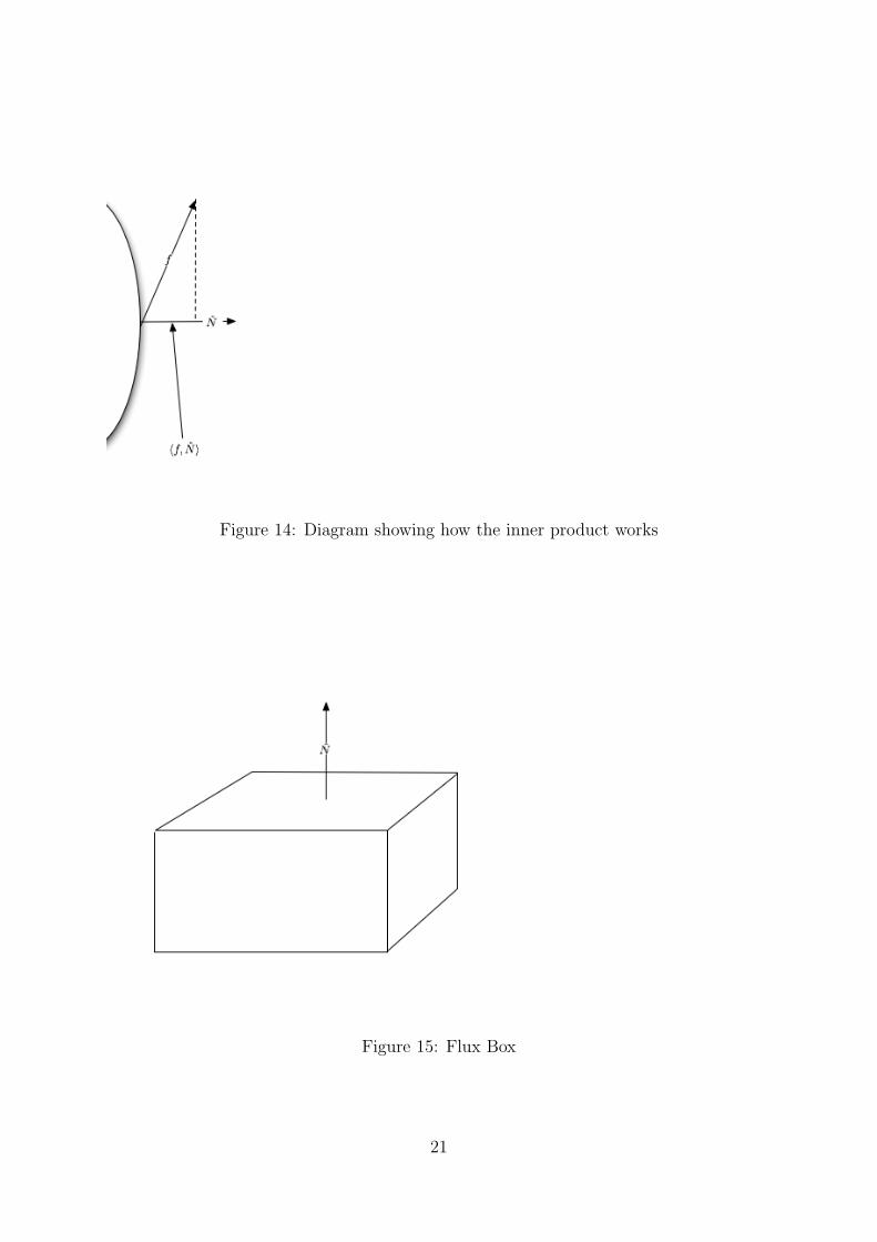
Figure 14: Diagram showing how the inner product works
Figure 15: Flux Box
21

∥∥∥∥∂r∂x × ∂r
∂x× ∂r
∂y
∥∥∥∥ =
∥∥∥∥∥∥ 1
00
× 0
10
∥∥∥∥∥∥ =
∥∥∥∥∥∥ 0
01
∥∥∥∥∥∥ = 1 (6.1)
∫st
〈f, N〉 =
∫ bx
ax
∫ by
ay
f3(x, y, tz)dydx
The flux through the bottom
N =
00−1
〈f, N〉 = f3 b2 changed a2∫
Sbottom
〈f, N〉 = −∫ bx
ax
∫ by
ay
f3(x, y, tz)dydx
Top+Bottom ∫ bx
ax
∫ by
ay
f3(x, y, b2)− f3(x, y, a2)dydx
=
∫ bx
ax
∫ by
ay
∫ bz
az
∂f3
∂z(x, y, z)dz︸ ︷︷ ︸
by FTC
dydx (6.2)
Similarly ∫Sleft∪Sright
〈f, N〉 =
∫ bx
ax
∫ by
ay
∫ bz
az
∂f1
∂x(x, y, z)dzdydx (6.3)∫
Sfront∪Sback
〈f, N〉 =
∫ bx
ax
∫ by
ay
∫ bz
az
∂f2
∂ydxdydz (6.4)
Taking the sum of equations 6.2, 6.3 and 6.4 we then get the total flux which is:∫δΩ
〈f, N〉 =
∫ bx
ax
∫ by
ay
∫ bz
az
∂f1
∂x+∂f2
∂y
∂f3
∂zdzdydx (6.5)
Definition 6.2 (Divergence). The divergence of a vector field f : Rn → Rn is divf :Rn → R
divf =n∑i=0
∂fi∂x
Alternative notations: ∇ · V , ∇−→V and ∇ · V
Remark 6.1. Scalar field to vector field
V : Rn → R→ gradV : Rn → Rn
f : Rn → Rn ⇔ f : Rn → R
22

Figure 16: Diagram showing f(x)× ε
Definition 6.3. Let V : Rn → R be a scalar field. The Laplacian of V is ∆V = div gradV(Scalar field)
gradV =
(∂V∂x1∂V∂xn
)⇒ div gradV =
n∑i=1
∂Vi∂ki
Alternative notations include: ∇ · ∇V , ∆V , ∇2V .
26/10/06
divf(x) =∑ ∂f
∂x(x)
Ω = [a1, b1]× [a2, b2]× [a3, b3] ∫Ω
〈f, N〉 =
∫divf(x)dx (6.6)
Remark 6.2. If Ω is a small box around a ∈ R3 then Ω = [a1 − ε, a1 + ε]× [a2 − ε, a2 +ε]× [a3 − ε, a3 + ε] Then ∫
Ω
div(x)dx ≈ divf(α)− Va(Ω)
⇒ divf(a) ∼=∫δΩ〈f, N〉V0(Ω)
Thus the divergence gives the outward flux per unit volume.
Remembering that divf(x) = ∇ · f
7 Gauss Divergence Theorem
Definition 7.1 (Divergence). The divergence of a C1 vector field f ⊆ R3 is:
divV = ∇ · V =3∑i=1
∂fi∂xi
(7.1)
23

Figure 17: Positive Divergence
Figure 18: Zero Divergence
Figure 19: Negative Divergence
24

Theorem 7.1 (Divergence Theorem). Let Ω ⊆ R3 be a bounded with a surface δΩ andoutward unit normals N . Let V : Ω ∪ δΩ→ R3 be continuously differentiable, then:∫
δΩ
〈V, N〉 =
∫Ω
divV (x)dx (7.2)
Remark 7.1. The theorem also works for n 6= 3 but one has to define the surface integral,n = 2δΩ is a line and
∫δΩ
is a (scalar) line integral.
Remark 7.2. divf(x)dx is just an iterated integral, alternative notation is:∫
ΩdivfdV (n =
3),∫
ΩdivfdA (n = 2).
Example 7.1. Box in R3 already done in example 6.1
Example 7.2. Ball of radius R in Rn
Ω = B(0, R) ⊆ Rn
δΩ = Shell of Sphere, N(x) =x
RLet:
f(x) = x⇒ divf(x) =∂x1
∂x1
+ · · ·+ ∂xn∂xn
= 1 + · · ·+ 1 = n
⇒∫B(0,R)
ndx =
∫δB(0, R)
⟨x,x
R
⟩∫δB(0,R)
R⇒ n× Volume of Ball = R× Surface Area of Ball
For n = 2 then VolB(0, R) = πR2 This means that the length of δB(0, R) = 2πR, forn = 3 the volume of the ball is 4
3πR3 And the surface area is 3
Rtimes that.
30/10/06
Sketch Proof of Divergence theorem.
1. As we covered in example 6.1, it is already true for boxes.
2. Therefore we can use the fact that it holds for boxes to suppose the theorem holdsfor Ω1,Ω2 as shown in figure 20, what about the region Ω1 ∪ Ω2? Then:∫
δΩ
⟨V, N
⟩=
∫δΩ1
⟨V, N
⟩+
∫δΩ2
⟨V, N
⟩Since the contribution form the shared boundary cancels as they are in oppositedirections, this is equal to:
=
∫Ω1
∇V +
∫Ω2
∇V =
∫Ω1∪Ω2
∇V
16
16I’m using nabla instead of div here as its easier
25

Figure 20: Diagram of 2 boxes for sketch proof of divergence theorem
3. For simple regions (in R2)
Ω is simple⇔ Ω =
(x, y)∣∣f(y) ≤ x ≤ g(y) ∀ y ∈ [a, b]
=
(x, y)∣∣f(x) ≤ y ≤ g(x) ∀x ∈ [c, d]
So a circle with a hole in the middle of it (like a wheel with a missing axle) isn’tsimple but if you cut it in half into a semi circle then it would be simple.17.
4. If we show Ω is simple then:∫Ω
∂V1
∂xdA =
∫ b
a
∫ g(y)
f(y)
∂V
∂x1
(x, y)dxdy =
∫ b
a
V1(f(y), y)−∫V1
(f(y), y)
)dy (7.3)
Flux of
(V1
0
)through the boundary, the region is shown in figure 21 The flux
γk(ψ) =
(g(y)y
)for y ∈ [a, b]
γ′k(ψ) =
(g′(y)
1
)Generally we know that
(xy
)⊥(−yx
)
N =1
‖γR‖
(g′(y)
1
)=
1√1 +
(g′(y)
)2
(g′(y)
1
)∫γk
⟨(V1
0
), N
⟩17In metric spaces language it is simple if it is topologically equivalent to a square
26

Figure 21: Diagram showing the region Ω with two boundary functions and two fluxfunctions.
1
‖γ′(y)‖
⟨(V1
0
),
(1
−g′(y)
)⟩∫ b
a
V11
‖γ′R(y)‖‖γ′R(y)‖dy
=
∫ b
a
V1
(g(y), y
)dy
Similarly for the LHS:∫γL
⟨(V1
0
), N
⟩= −
∫ b
a
V1
(f(y), y
)dy
As ∫γT
⟨(V1
0
), N
⟩=
∫γB
⟨(V1
0
), N
⟩= 0
⇒∫ b
a
V1
(g(y), y
)− V1
(f(y), y
)dy
=
∫Ω
∇(V1
0
)dA
This then shows that the theorem holds for V =
(V1
0
). If we then use f and g
instead of f and g, and if we interchange x and y we get that:∫δΩ
⟨(0V2
), N
⟩=
∫Ω
∇(
0V2
)dA
Adding these results together completes the proof.
27

8 Integration by Parts
If the following hold:Ω ⊂ R, Ω18 = Ω ∪ δΩ
Proposition 8.1. Then for f : Ω→ R where f is C1. Then:∫Ω
∂f
∂x=
∫δΩ
f · N19 (8.1)
Proof. Let v = (f, 0, 0) then:
÷v =∂f
∂x1
〈v, N〉 = fN1
⇒ If the divergence thoerem is applied to the special vector field v given in equation 8.1,then using (0, f, 0) and (0, 0, f) we can also show it for i = 2, 3.
Remark 8.1. The full divergence theorem (theorem 7.1) can be derived from equation8.1
Proposition 8.2. Integration by parts:∫ b
a
uv′dx =[uv]ba−∫ b
a
u′vdx (8.2)
Then applying equation 8.1 to f = gh we get:
∂f
∂xi=
∂g
∂xih+ g
∂h
∂xi
⇒∫
Ω
∂g
∂xi= −
∫Ω
g∂h
∂xi+
∫δΩ
ghNi
Proposition 8.3. Let g : Ω→ R be twice continuously differentiable, i.e. apply proposi-tion 8.1to f = ∂g
∂xi
⇒∫
Ω
∂2g
∂x2i
=
∫δΩ
∂y
∂xiNi
Summing up over i then gives ∫Ω
∆g =
∫δΩ
〈∇g, N〉 (8.3)
Proposition 8.4. Applying proposition 8.2 with g = ∂f∂xi
and sum over i we get:∫Ω
∆fh = −∫
Ω
〈∇f,∇h〉+
∫δΩ
g〈∇f, N〉
〈÷gradf, h〉 − 〈gradf, gradh〉 (8.4)
18This means the closure of Ω as in metric spaces19in the lectures described as Ni for i = 1, 2, 3.
28

(a, c) (b, c)
(b, d)(a, d)
Ω γR
γT
γL
γB
T
Figure 22: A rectangle Ω
8.1 Application
Temperature distribution in steady state. Ω ⊆ R3 a piece of material. Fix temperaturef(x) ∀x ∈ δΩ. In steady state the temperature solves:
∆T (x) = 0 ∀x ∈ ΩT (x) = f(x) ∀x ∈ δΩ
The existence of a solution s of this is a difficult question.
8.2 Uniqueness
Assume T and T are solutions, then D = T − T solves
∆D = ∆T −∆T = 0− 0 = 0 ∀x ∈ δΩ
D(x) = T (x)− T (x) = f(x)− f(x) = 0 ∀x ∈ δΩ
Using proposition 8.4 we get:∫Ω
∆D︸ ︷︷ ︸=0
= −∫
Ω
〈∇D,∇D〉+
∫δΩ
D〈∇D, N〉
∫Ω
‖∇D‖2 = 0
⇒ ∇D(x) = 0 ∀x ∈ Ω
⇒ D is constant and D = 0 at the boundary, therefore T = T so T is a unqiue solution.
9 Green’s Theorem
20
20This section is done by Matthew Pusey
29

Consider a function f : R2 → R2 and a rectangle Ω = [a, b]× [c, d] with boundary unittangent vectors T in the anticlockwise (positive) direction. This is shown in Figure 22.
On the right side, γR. which is the line segment from (b, c) to (b, d):∫γR
⟨f, T
⟩=
∫ d
c
⟨f(b, y),
(01
)⟩dy =
∫ d
c
f2(b, y)dy
The remaining sides, γL, γB, γT are similar (but take care with signs):∫γL
⟨f, T
⟩= −
∫ d
c
f2(a, y)dy
∫γB
⟨f, T
⟩=
∫ b
a
f1(x, c)dx∫γT
⟨f, T
⟩= −
∫ b
a
f1(x, d)dx
Summing these gives:∫∂Ω
⟨f, T
⟩=
∫ d
c
f2(b, y)− f2(a, y)dy +
∫ b
a
f1(x, c)− f1(x, d)dx
The Fundamental Theorem of Calculus then gives:
=
∫ d
c
∫ b
a
∂f2
∂x(x, y)dxdy −
∫ b
a
∫ d
c
∂f1
∂y(x, y)dydx
=
∫ d
c
∫ b
a
∂f2
∂x− ∂f1
∂ydydx
Definition 9.1 (2-D curl). For f : R2 → R2, the curl of f is given by:
curl f(x) =∂f2
∂x− ∂f1
∂y
Remark 9.1.∫∂Ω
⟨f, T
⟩is the circulation around Ω. By talking small boxes we find that
curl f(x) is the circulation of f around x.
Sometimes you can see what the curl is:
Example 9.1.
v(x, y) =
(−yx
)This is shown in figure 23.
curl v(x, y) = 1− (−1) = 2
30

Figure 23: Diagram showing a vector field.
Figure 24: Diagram showing a vector field.
31
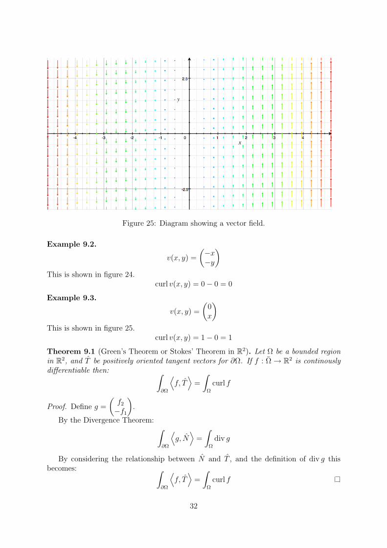
Figure 25: Diagram showing a vector field.
Example 9.2.
v(x, y) =
(−x−y
)This is shown in figure 24.
curl v(x, y) = 0− 0 = 0
Example 9.3.
v(x, y) =
(0x
)This is shown in figure 25.
curl v(x, y) = 1− 0 = 1
Theorem 9.1 (Green’s Theorem or Stokes’ Theorem in R2). Let Ω be a bounded regionin R2, and T be positively oriented tangent vectors for ∂Ω. If f : Ω→ R2 is continouslydifferentiable then: ∫
∂Ω
⟨f, T
⟩=
∫Ω
curl f
Proof. Define g =
(f2
−f1
).
By the Divergence Theorem: ∫∂Ω
⟨g, N
⟩=
∫Ω
div g
By considering the relationship between N and T , and the definition of div g thisbecomes: ∫
∂Ω
⟨f, T
⟩=
∫Ω
curl f
32
10 Stokes Theorem (curls in R3)
6/11/06
Theorem 10.1. Let S ∈ R3 be a bounded surface with N as unit normals of S, andT unit tangent vectors to the boundary line δS. Let f : S ∪ δS → R3 be continuously
differentiable. If⟨N , T
⟩is positively oriented, then:∫
S
⟨curlf, N
⟩−∫δS〈f, T 〉 = 0
Remark 10.1. Positive oriented means that if N points upwards, the tangent vectorsare anti-clockwise,and if N points downwards, the tangent vectors are clockwise. (i.e. theright hand rule applies).
Remark 10.2. In R3, curl = ∇× f ∂2f3 − ∂3f2
∂3f1 − ∂1f3
∂1f2 − ∂2f1
Remark 10.3. In R2 curlg = ∂1g2 − ∂2g1
Example 10.1. For g : R2 → R2 and f : R3 → R3
f(x, y, z) =
g1(x, y)g2(x, y)
0
curlf =
0− 00− 0curl g
= curl g
For Ω ⊆ R× R× 0 and Ω′ ⊂ R2 (the x-y plane), we then get
∫Ω′
curl g =
∫Ω
⟨curl f,
001
⟩
And so by Stoke’s theorem
=
∫δΩ
⟨f, T
⟩=
∫δΩ′
⟨g, T
⟩Example 10.2. S = (x, y, z)
∣∣z = x2 + y2, z ≤ 4 This is then of the form
r(x, y) =
xy
x2 + y2
33

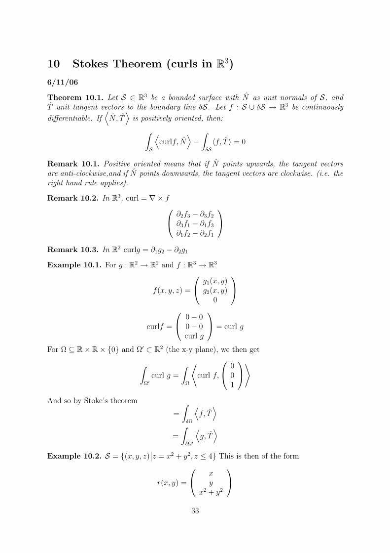
Figure 26: Graph showing a hemispherical bowl, the top should be smooth at the pointof the peaks, but grapher can’t draw it correctly.
N(x, y, z) = ∇(2− x2 − y2) =
−2x−2y
1
= δS
Is then parameterised by:
γ(t) =
2 cos t2 sin t
4
, t ∈ [0, 2π]
A diagram is shown in figure 26 Now let
f :=
yx2
3z2
∫δS
⟨f, T ,=
⟩∫ 2π
0
⟨ 2 sin t4 cos2 t3 · 16
· −2 sin t−2 cos t
0
⟩ = −4π
curl f =
0− 00− 0
2x− 1
∫S〈curl f, N〉 =
∫∫ 00
2x− 1
· −2x−2y
1
dsdt =
∫∫2x− 1dsdt
∫∫B(0,2)
2x− 1dxdy∫∫B(0,2)
2xdxdy −∫∫
B(0,2)
1dxdy
34

Figure 27: Graph showing region being ”lifted” to R3
0− 4π = −4π (as we got before!)∫S
⟨curl f, N
⟩=
∫δS
⟨f, T
⟩Proof of theorem 10.1. We ”lift” Green’s theorem from R2 to R3, this is shown in figure27. Now we parameterise δΩ by γ : [a, b] → R2. ⇒ δS is parameterised by r
(γ(u)
)=
u ∈ [a, b]. Tangent TS
(r(γ(u)
))′∂r
∂s
∂γ1
∂u+∂r
∂t
∂γ2
∂u
⇒∫∂S〈f, T 〉
=
∫ b
a
⟨f(γ(u)
),∂r
∂s
∂γ1
∂u+∂r
∂t
∂γ2
∂u
⟩=
∫ b
a
⟨( ⟨f, ∂r
∂s
⟩⟨f, ∂r
∂t
⟩ ) , γ′(u)
⟩du∫
δΩ
⟨( ⟨f, ∂r
∂s
⟩⟨f, ∂r
∂t
⟩ ) , TΩ
⟩(10.1)
Similarly ∫S
⟨curl f, N
⟩
35

=
⟨curl f
(r(s, t)
),∂r
∂s× ∂r
∂t
⟩dsdt
Omitting the middle (Chain rule + hard work)
=
∫∫Ω
curl
( ⟨f, ∂r
∂s
⟩⟨f, ∂r
∂t
⟩ ) (10.2)
By Green’s theorem equations 10.1 and 10.2 are equal. When showing the equality of10.2 we have to keep track of many (about 48) terms, in later courses we find differentialforms useful for this.
Remark 10.4. If f : R3 → R3 is a gradient then:∫S
⟨curl f, N
⟩=︸︷︷︸
Stokes
∫δΩ
⟨f, T
⟩= 0
∫γ
⟨f, T
⟩= V (b)− V (a)
by the FTC for gradient vector fields.
curl grad v =
∂∂x∂∂y∂∂z
× ∂v
∂x∂v∂y∂v∂z
=
(∂2v
∂y∂z− ∂2v
∂z∂y
)= 0
Curl of gradient vector fields is always zero. Similarly f : R3 → R3 with f = curl v we
get∫δΩ
⟨f, N
⟩=∫
Ωdiv f , div curl v = · · · = 0
11 Spherical Coordinates
Skipped, will be a PDF of most of this topic included later.
12 Complex Differentation
21
The aim of this section is to understand calculus for functions f : C→ C, and its linkto vector analysis.
Definition 12.1 (Complex Numbers). The complex numbers are defined by:
C =x+ iy
∣∣ x, y ∈ R, i2 = −1
Clearly, there is a one-to-one correspondence between C→ C functions and R2 → R2
functions:f : C→ C ↔ (u, v) : R2 → R2
Where f(x+ iy) = u(x, y) + iv(x, y).
36

Re
Im
z
rx
y
φ
1
Figure 28: Planar representation of a real number z
12.1 Basic properties of Complex Numbers
z = x+ iy
z = r cosφ+ ir sinφ
r =√x2 + y2 = |z|
φ = arctan(yx
)= arg(z)
Addition
(x1 + iy1) + (x2 + iy2) = (x1 + x2) + i(y1 + y2)
Multiplication
(x1 + iy1)(x2 + iy2) = (x1x2 − y1y2) + i(y1x2 + x1y2)
The meaning of this is clearer in polars, for example if z = r cosφ + ir sinφ and w =s cosψ + is sinψ then:
zw = rs cos(φ+ ψ) + irs sin(φ+ ψ)
Complex conjugation
z = x+ iy ⇐⇒ z = x− iy
12.2 Limits
Definition 12.2 (Limits). For zn, z ∈ C:
zn → z ⇐⇒ |zn − z| → 0
21The next two sections are done by Matthew Pusey
37

By the definition of |z|:
zn → z ⇐⇒√
(xn − x)2 + (yn − y)2 → 0 ⇐⇒ xn → x and yn → y
Lemma 12.1. If zn → z and wn → w then:
zn + wn → z + w
znwn → zwznzw→ z
wif w 6= 0
Sketch proof. Exactly as for R, but need to avoid inequalities in C, which make no sense.Still have that:
|zw| = |z||w|
|z + w| ≤ |z|+ |w|
And can define an open ball:
B(z, ε) = z′ ∈ C : |z − z′| ≤ ε
So that:zn → z ⇐⇒ ∀ε > 0∃N ∈ N such that ∀n ≥ N, zn ∈ B(z, ε)
12.3 Continuity & Differentiation
Definition 12.3 (Continuity). A function f : D → C for D ⊂ C is continuous at z ∈ Dif: B(z, ε) ⊆ D for some ε > 0 and:
zn → z =⇒ f(zn)→ f(z)
Note: This must hold for all sequences (zn) with zn → z. We say f is continuous on Dif f is continuous at every z ∈ D.
Remark 12.1. f is continuous at z ⇐⇒ ∀ε > 0, ∃δ > 0 such that:
|zn − z| < δ =⇒ |f(zn)− f(z)| < ε
Definition 12.4 (Differentiation). A function f : D → C with D ⊂ C is differentiableat z ∈ D if
f ′(z) = limh→0
f(z + h)− f(z)
h
exists. Note that this means
f ′(z) = limn→∞
f(z + hn)− f(z)
hn
exists for any hz → 0.
38

Example 12.1.f(z) = z
It’s clear thatzn → z =⇒ f(zn)→ f(z)
So f is continuous.
f(z + h)− f(z)
h=z + h− z
h= 1→ 1 =⇒ f ′(z) ≡ 1
Example 12.2.f(z) = z
zn → z =⇒ xn → x, yn → y
=⇒ xn → x,−yn → −y=⇒ f(zn)→ f(z)
So f is continuous. But it is not differentiable, since the limit
limh→0
f(z + h)− f(z)
h= lim
h→0
h
h
does not exist. For example, with hn = 1n
it tends to 1 but with hn = in
it tends to -1.
Lemma 12.2. Let f, g : D → C, with D ⊆ C, be continuous (and differentiable) at z.Then f + g, fg and f
g(g 6= 0) are also continuous (and differentiable).
Let f(x+ iy) = u(x, y) + iv(x, y). Then certainly:
f continuous ⇐⇒ uv continuous
But:f differentiable ⇐⇒ uv differentiable
does not hold in general.
13 Complex power series
Definition 13.1.∑∞
n=0 cn converges (to c) if:
SN =N∑n=0
cn
converges (to c).
As in R, we have the Cauchy criterion for a sequence (zn):
∀ε > 0,∃N ∈ N such that ∀m,n ≥ N, |zm − zn| < ε
Loosely speaking, a sequence is Cauchy if “|zm − zn| → 0 as m,n → ∞”. It is easyto show that if (zn) is Cauchy its real and imaginary parts are Cauchy, so the sequenceconverges in C since the parts must converge in R.
39

Lemma 13.1. If |fn(z)| ≤Mn∀z ∈ D and∑∞
n=0Mn <∞ then
f(z) =∞∑n=0
fn(z)
converges for all z ∈ D. Also, if all the fn are continuous then so is f .
Proof. Let SN =∑N
k=0 fk(z). Then, assuming without loss of generality that m > n:
|Sm(z)− Sn(z)| =
∣∣∣∣∣m∑
k=n+1
fk(z)
∣∣∣∣∣≤
∣∣∣∣∣m∑
k=n+1
Mk
∣∣∣∣∣≤
∣∣∣∣∣∞∑
k=n+1
Mk
∣∣∣∣∣→ 0 as n→∞
Theorem 13.2 (Power series). Let (cn) be a sequence in C, and define:
f(z) =∞∑n=0
cnzn
Then there exists some R ∈ [0,∞] such that f(z) converges if |z| < R, and doesn’tconverge if |z| > R.
Notes:
1. f may or may not converge when |z| = R.
2. A similar theorem holds in R and the proof carries over.
3. The theorem can be applied repeatedly.
4. f is C∞ on B(0, R), with:
∂k
∂zkf(z) =
∞∑n=k
n(n− 1) · · · (n− k + 1)cnzn−k
5. If f(z) converges on B(0, R) then g(z) =∑∞
n=0 cn(z − a)n converges on B(a,R).
To calculate R we can use the ratio test.
Lemma 13.3 (Ratio test). If
|zn+1||zn|
→ L ∈ [0,∞]
then∑∞
n=0 zn converges if L < 1 and diverges if L > 1.
40

Sketch proof. Observe that ∣∣∣∣∣m∑
k=n+2
zk
∣∣∣∣∣ ≤m∑
k=n+1
|zk|
and use the result on R + Cauchy
Example 13.1.
f(z) =∞∑n=0
(3 + i)(2i)n︸ ︷︷ ︸cn
(z + i)n
|zn+1||zn|
=
∣∣∣∣(2i)n+1(z + i)n+i
(2i)n(z + i)n
∣∣∣∣ = |2i(z + i)| = |2i||z + i|
= 2|z + i| → 2|z + i| = L
So when |z + i| < 12, f(z) converges, and when |z + i| > 1
2, f(z) doesn’t converge. This
gives R = 12.
Example 13.2.
f(z) =∞∑n=1
zn
n
|zn+1||zn|
=
∣∣∣∣ zn+1n
(n+ 1)zn
∣∣∣∣ =n
n+ 1|z| → |z| = L
This gives R = 1.What about when |z| = 1? f(1) diverges, f(−1) converges to log 2. In general this is
a hard problem.
Definition 13.2 (Common power series).
ez = exp(z) =∞∑n=0
zn
n!
cos(z) =∞∑n=0
1
(2n)!z2n(−1)n
cosh(z) =∞∑n=0
1
(2n)!z2n
sin(z) =∞∑n=0
1
(2n+ 1)!z2n+1(−1)n
sinh(z) =∞∑n=0
1
(2n+ 1)!z2n+1
Lemma 13.4.
sin(z) =eiz − e−iz
2icos(z) =
eiz + e−iz
2
sinh(z) =ez − e−z
2cosh(z) =
ez + e−z
2
41

Proof. Use the power series. For example, to prove the one for cos(z):
eiz + e−iz
2=
1
2
∞∑n=0
((iz)n
n!+
(−iz)n
n!
)
=1
2
∞∑n=0
zn((i)n + (−i)n)
n!
The numerator here is 2in if n is even, and 0 is n is odd. Therefore it equals:
∞∑k=0
z2k
2k!(−1)k = cos(z)
Example 13.3.
sin(iy) =e−y − ey
2i= i
ey − e−y
2= i sinh(y)
14 Holomorphic Functions
Let f(x+ iy) = u(x, y) + iv(x, y), for h = ε+ i · 0
limε→0
u(x+ ε, y)− u(x, y)
ε+ i lim
ε→0
v(x+ ε, y)− v(x, y)
ε=∂u
∂x+ i
∂v
∂x
For h = 0 + iε.
f ′(z) = (−i) limε→0
u(x, y + ε)− u(x, y)
(−i)ε+ i lim
ε→0
v(x, y + ε)− v(x, y)
iε
f is only differentiable if∂u
∂x+ i
∂v
∂x= −i∂u
∂y+∂v
∂y
Definition 14.1 (The Cauchy Riemann equations). A complex function f(x + iy) =u(x, y) + iv(x, y) is differentiable if and only if:
∂u
∂x=∂v
∂y
∂v
∂x= −∂u
∂y
Theorem 14.1. Consider f : D → C, D ⊆ C with:
f(x+ iy) = u(x, y) + iv(x, y)
1. If f is differentiable at (x0, y0) then∂u∂x, ∂u∂y, ∂v∂x, ∂v∂y
exist at (x0, y0) and the Cauchy
Riemann equations (definition 14.1) hold at (x0, y0).
42

2. If ∂u∂x, ∂u
∂y, ∂v
∂x, ∂v
∂yand are continuous in a small Ball around (x0, y0) then f is
differentiable at (x0, y0) with z0 = x0 + iy0 with
f ′(z0) =∂u
∂x+ i
∂v
∂x=∂v
∂y− i∂u
∂y
Example 14.1 (Example to show the difference between points 1 and 2). f(z) = z3
must be differentiable everywhere.
f(x+ iy) = (x+ iy)3
= x3 + 3x(iy)2 + 3x2(iy) + (iy)3
= x3 − 3xy2︸ ︷︷ ︸u(x,y)
+i (3yx2 − y3)︸ ︷︷ ︸v(x,y)
∂u
∂x= 3x2 − 3y2 (14.1)
∂v
∂y= 3x2 − 3y2 (14.2)
As you can see equations 14.1 and 14.2 are the same.
∂u
∂y= −6xy (14.3)
plv
∂x= 6xy (14.4)
As you can see equations 14.3 and 14.4 are the same.
21/11/06
Example 14.2 (Hard example).
f(x+ iy) = x2 + iy2
∂u∂x
= 2x, ∂v∂y
= 2y, (these are in general not equal so the function isn’t differentiable.∂v∂x
= 0, ∂u∂y
= 0 (these are equal and have to be equal for differentiability.)Therefore f is only differentiable if x = y.
Definition 14.2. If a function f : D → C where D ⊆ C is holomorphic at z0 ∈ D iff is differentiable for all z ∈ B(z0, ε) for some ε > 0. f is holomorphic on D if it isholomorphic ∀ z ∈ D.
Remark 14.1. The aim is to apply Vector Analysis to this problem.
43

If f(x+ iy) = u+ iv is holomorphic then we define:
f(x, y) =
(u(x, y)−v(x, y)
)For R2 → R2, then
∇ · F (x, y) =∂u
∂x− ∂v
∂y=︸︷︷︸
by Cauchy Riemann
0
and
curl F (x, y) = −∂u∂y− ∂v
∂x= 0
∂F2
∂x− ∂F
∂y22
15 Complex Integration
Theorem 15.1. Consider a parameterised curve γ[a, b]→ C
γ(t) = x(t) + iy(t)
⇒ γ′(t) = x′(t) + iy′(t)
Remark 15.1. The Divergence theorem and Green’s theorem might be useful here.
Definition 15.1. For F : D → C:∫γ
f =
∫ b
a
f(γ(t)
)γ′(t)dt
=
∫ b
a
Re(f(γ(t)
)γ′(t)
)dt+ i
∫ b
a
Im(f(γ(t)
)γ′(t)
)dt
Example 15.1.f(x+ iy) = x2 + iy
γ(t) = t(1 + i) for t ∈ [0, 1]∫γ
f =
∫ 1
0
t2 + it2(1 + i)dt
=
∫ 1
0t2 + it2 + it2 − t2dt∫ 1
0
2it2dt
= 2i
∫ 1
0
t2dt
= 2i
[t3
3
]1
0
=2i
322I don’t understand this.
44

Remark 15.2. If γ and γ parameterise the same path in the same direction, then if:∫γf =
∫γf . If the direction is reversed then
∫γf = −
∫γf .
Example 15.2. Integrate f(z) = z around δB(i, 2). Since eit = cos t+ i sin t, we can useγ(t) = 2eit + i to parameterise δB(i, 2).∫
γ
f =
∫ (2eit + i
)2ieitdt
∫ 2π
0
(−i+ 2e−it + i)2ieitdt
=
∫ 2π
0
2eit + 4idt
=
[2eit
i
]2π
0
+ 8πi
= 8πi
∫γ
f =
∫ b
a
f(γ(t)
)γ′(t)dt
∫ 2π
0
eitdt =
[eit
i
]t=2π
t=0
23
Theorem 15.2 (Fundamental Theorem of Calculus for Complex Integrals). Let f : D →C be holomorphic for D ⊆ C, γ : [a, b]→ C then∫
γ
f ′ = f(γ(b)
)− f
(γ(a)
)Proof. ∫
γ
∂f
∂z=
∫ b
a
∂f
∂z
(γ(t)
)∂γ∂t
(t)dt∫ b
a
∂
∂t
(f(γ(t)
))dt = f
(γ(b)
)− f
(γ(a)
)This last statement is true by applying the real Fundamental theorem of calculus to
Re(f(γ(t)
)and Im
(f(γ(t)
))Remark 15.3. If f ′ = 0 and f is over a connected region24, then f is constant.
23This doesn’t make much sense tbh24As in metric spaces
45

16 Cauchy’s theorem
For γ : [a, b]→ Cγ(t) = x(t) + iy(t)
f(x+ iy) = u(x, y) + iv(x, y)
We get that ∫γ
f =
∫ b
a
u(x(t), y(t)
)+ iv
(x(t), y(t)
)(x′(t) + iy′(t)
)dt
=
∫ b
a
(ux′ − vy′)dt+ i
∫ b
a
(uy′ + vx′)dt
=
∫ b
a
(u−v
)·(x′
y′
)dt+ i
∫ b
a
(u−v
)·(
y′
−x′)dt
=
∫γ
⟨F, T
⟩+ i
∫γ?????
⟨F, N
⟩where F (x, y) =
(u(x, y)−v(x, y)
)Now by using Green’s theorem (9.1) and the divergence
theorem (7.1)
Theorem 16.1 (Cauchy). Let a function f : D → C, D ⊆ C be holomorphic and Ω ⊆ Da region with a boundary of δΩ. If γ is a parameterisation of δΩ then:∫
γ
f = 025
Proof. ∫γ
f︸︷︷︸C
=
∫γ
⟨F, T
⟩︸ ︷︷ ︸
R2
+i
∫γ
⟨F, N
⟩︸ ︷︷ ︸
R2∫γ
⟨F, T
⟩=︸︷︷︸
Green
±∫
Ω
curl F =︸︷︷︸Cauchy-Riemann
0
∫γ?????
⟨F, N
⟩=︸︷︷︸
Divergence
±∫
Ω
div F =︸︷︷︸Cauchy-Riemann
0
Remark 16.1. The theorem holds for more general curves so as the curve in figure 29and in this case ∫
γ
f =
∫γ1
f +
∫γ2
f = 0
However the curve has to be simple, i.e. it must be possible to contract the curve to apoint, so for example it wouldn’t apply to the curve in figure 30, as Ω * D
25This is the main result of the Complex Analysis part if the course
46

Figure 29: A more general curve to which Cauchy’s theorem applies.
Figure 30: A region and domain which it doesn’t apply
47

Figure 31: Complex circle of radius π.
Example 16.1.
f(z) =1
z, γ(t) = Reit t ∈ [0, 2π]
⇒∫γ
f =
∫ 2π
0
1
ReitiReitdt = i
∫ 2π
0
1dt = 2πi 6= 0
27/11/06
Proposition 16.2. We have seen that:∫δB(0,R)
1
1 + ezdz = 0 ∀Real numbers
Proof.1 + ez = 0⇔ ez = −1
This is shown in figure 31. Now we know that |ez| = ex and arg(ez) = y and ez = −1which implies that x = 0, y = (2n+1)π, ∀n ∈ Z. This means that for a ball of radius lessthan π, i.e R ∈ [0, π) then the value of the integral is zero. This means f is holomorphicon any complex circle with R < π.
17 Cauchy Integral Formula
Let γ be the boundary of a connected region Ω ⊆ C with positive orientation.
Remark 17.1 (Idea 1). 26 We can deform γ without changing the integral∫γf . As we
26These are really ideas but I using remarks instead
48

Figure 32: Diagram showing the region bounded by a curve γ, and a second curve γsplitting it into two pieces.
can see in figure 32 if there are a few points in the region bounded by gamma which aren’tholomorphic we can split the region into two pieces without changing the integral with asplit off region, bounded by the curve γ. If f is holomprohic on and between γ and γ,then if κ is the part of γ and γ bounding this new region then∫
κ
f = 0
Also ∫γ
f −∫γ
f =
∫f −
∫f
27 ∫simple loop
f = 0
Remark 17.2 (Idea 2). If f is holomorphic on and inside γ except for a finite numberof points z1, . . . , zn, this is shown in figure 33 and leads to what is shown in 34.∫
γ
f =n∑i=1
∫δB(zi,ε)
f
∀ ε > 0 small enough so that the balls don’t overlap.
27check original notes
49

Figure 33: Diagram showing the integral inside a curve γ
Figure 34: Integrals around the non homomorphic points.
50

Remark 17.3 (Idea 3). If:
f(z) =∞∑n=0
anzn
converges on B(0, R), R > 0, then:∫δB(0,ε)
f(z)
zdz =
∫δB(0,ε)
a0
z+ a1 + a2z + · · ·︸ ︷︷ ︸
Holomorphic
dz
= a0 2πi︸︷︷︸As in example
+ 0︸︷︷︸Cauchy
Similarly ∫δB(0,ε)
f(z)
zndz =
∫a0
zn+ · · ·︸ ︷︷ ︸
zero as primitive by FTC
+an−1
z+ an + an+1z + · · ·︸ ︷︷ ︸
Holomorphic
∂
∂zz1−k = (1− k)zk (except for k = 1)
⇒∫
a0
zn+ · · ·+ an−2
z2dz =︸︷︷︸
by the FTC
0
⇒∫δB(0,R)
f(z)
zn= 0︸︷︷︸
FTC
+an−12πi+ 0︸︷︷︸Cauchy
28/11/06
Theorem 17.1 (Cauchy Integral Formula). Let γ be the boundary of a connected region.Let f be holomorphic on and inside γ.∫
γ
f(z)
z − z0
= 2πif(z0) ∀ z0 inside γ
Remark 17.4. Holomorphic functions are special, the values of f along γ completelydetermine the values of f inside γ.
Lemma 17.2. ∣∣∣∣∫ b
a
x(t) + iy(t)dt
∣∣∣∣ ≤ ∫ b
a
|x(t) + y(t)|dt
Proof. If: ∫ b
a
x(t) + iy(t)dt ∈ R∣∣∣∣∫ b
a
x(t) + iy(t)
∣∣∣∣ dt =
∣∣∣∣∫ b
a
x(t)+
∣∣∣∣ dt ≤︸︷︷︸by Analysis 3
∫ b
a
|x(t)|dt ≤∫ b
a
|x(t) + iy(t)|dt
51
Generally ∫ b
a
x(t) + iy(t)dt = reiθ forr,∈ R, θ ∈ [0, 2π]
r = e−iθ∫ b
a
x(t) + iy(t)dt =
∫ b
a
eiθ(x(t) + iy(t)
)dt
=
∣∣∣∣∫ b
a
eiθ(x(t) + iy(t)
)dt
∣∣∣∣ ≤ ∫ b
a
∣∣eiθ∣∣ ∣∣x(t) + iy(t)∣∣dt =
∫ b
a
1 ·∣∣x(t) + iy(t)
∣∣dtRemark 17.5. If |f(z) ≤M on a curve γ then:∣∣∣∣∫
γ
f
∣∣∣∣ =
∣∣∣∣∫ b
a
(f(γ(t)
)γ′(t)
)∣∣∣∣ ≤ ∫ b
a
< M |γ′(t)|dt = M
∫ b
a
|γ′(t)|dt
Therefore this means that M is the length of γ.
Proof of theorem 17.1. By deforming γ∫γ
f(z)
z − z0
=
∫δB(z0,ε)
f(z)
z − z0
dz
=
∫δB(z0,ε)
f(z0)
z + z0
dz︸ ︷︷ ︸(a)
+
∫δB(z0,ε)
f(z)− f(z0)
z − z0︸ ︷︷ ︸(b)
dz (17.1)
Then part a of equation 17.1 is equal to:
(a) = f(z0)
∫δB(0,ε)
1
zdz = f(z0)2πi
Then the absolute value of part b of equation 17.1 is:
|(b)| ≤ max
∣∣∣∣f(z)− f(z0)
z − z0
∣∣∣∣ · 2πε ≤ (|f ′(z0)|+ 1)2πε (17.2)
then for small epsilon the right hand side of equation 17.2 tends to zero as ε ↓ 0, thereforepart b of equation 17.1 tends to zero. 28
Example 17.1.
∫sin z
z − idz =
0 If i is outside γ
2πi sin i If i is inside γ? If i is on the curve though we are lost.
This is shown in figure 35
29
28Not convinced complete.29Check complete.
52

Figure 35: Diagram showing the three possible cases for the curve γ
53

Figure 36: Diagram showing the integral of γ split into four pieces.
18 Real Integrals
Aim to find the integral of: ∫ +∞
−∞
sinx
xdx (18.1)
As sinxx→ 1 as x→ 0 (by L’Hopital as cosx
1→ 1) So the function is defined everywhere.
A diagram of the curve γ which we will use to integrate equation 18.1 is shown in figure36. The strategy for solving this integral is to Integrate f along γ by Cauchy’s theorem(16.1). As we known that f is holomorphic in the region enclosed by γ in figure 36 thenwe know that: ∫
γ1
f +
∫γ3
f +
∫γ2
f +
∫γ4
f︸ ︷︷ ︸what we want
= 0 (18.2)
30/11/06 To solve equation 18.1 we find f over γ1 and γ3.
f(z) =eiz
z
Equation 18.2 oviously then leads to:∫γ2
f +
∫γ4
f =
∫ −ε−R
eix
xdx+
∫ R
ε
eix
xdx
54

=
∫ −ε−R
cosx+ i sinx
xdx+
∫ R
ε
cosx+ i sinx
xdx
As since cos is an even function, and x is odd.
cos(−x)
−x= −cosx
x
→ε↓0
i
∫ R
−R
sinx
xdx
From Cauchy’s theorem as we showed in equation 18.2∫γ1
f +
∫γ2
f + intγ3f +
∫γ4
f = 0
→ i
∫ R
−R
sinx
xdx = lim
ε↓0
(∫γ1
f +
∫γ3
f
)So: ∫
γ3
f =
∫γ3
1
zdz︸ ︷︷ ︸
(a)
+
∫γ3
eiz − 1
zdz︸ ︷︷ ︸
(b)
(18.3)
Now (a) = −iπ by question 2.2 of sheet 4.
|(b)| ≤ maxγ3
∣∣∣∣eiz − 1
z
∣∣∣∣ Length of γ3
≤ Cπε where C is a constant. Which tends to zero as ε→ 0.
eiz − 1
z= i
eiz − e0
iz⇒ ie′(0)
30 This∫γ3f → −πi as ε ↓ 0.
Now we claim that∫γ1→ 0 as R → ∞ This is because γ1(t) = Reit, t ∈ [0, π]
= R(cos t+ i sin t) ∣∣∣∣∫ π
0
eiR(cos t+i sin t)
ReitiReit
∣∣∣∣≤∫ π
0
∣∣eiR(cos t+i sin t)∣∣dt =
∫ π
0
e−R sin tdt (18.4)
So as sin t is positive over 0, π and it is symmetric along π2. Equation 18.4 then becomes:
= 2
∫ π2
0
e−R sin tdt (18.5)
As on[0, π
2
]sin t ≥ t
π2
So therefore equation 18.5 then is less than
(18.5) ≤ 2
∫ π2
0
e−Rtπ/2 = 2
∫ π2
0
e−2Rtπ
30not totally sure why last point holds
55

=−π2R· 2
(e− 2Rπ/2
π − e−2R·0π
)= − π
R
(e−R − 1
)= π
R
(1− e−R
)→ 0 as R→∞ By Cauchy’s Theorem as R→∞
i
∫ +∞
−∞
sinx
xdx︸ ︷︷ ︸
γ2,γ4
+ 0︸︷︷︸γ1
− iπ︸︷︷︸γ3
= 0
19 Power Series for holomorphic functions
Theorem 19.1. Suppose f : D → C and D ⊆ C is holomorphic, then:
f =∞∑r=0
arzr
where∑∞
r=0 ar is a convergent power series on any ball B(a,R) ⊆ D
Remark 19.1. If f is holomorphic implies that f is a power series so f is C∞
Theorem 19.2. ∫γ
f(z)
zdz = 2πf(0)
This is assuming that f : D → C is holomorphic, B(a,R) ⊆ D (An image of this isshown in figure 37). Together they imply that f is equal to a power series on B(a,R)
Proof. We can assume (without loss of generality) that a = 0 by shifting everything tothe origin. Then for every 0 < r < R
f(0) =1
2πi
∫δB(0,r)
f(z)
zdz ∀z0 ∈ B(0, R) (19.1)
If z0 ∈ δB(0, r) then: ∣∣∣z0
z
∣∣∣ < 1⇒ 1
z − z0
=1
z
1
1− z0z
=1
z
∞∑n=0
(z0
z
)n
⇒ f(z0) =1
2πi
∫δB(0,R)
f(z)1
z
∞∑n=0
(z0
z
)n=∞∑n=0
(1
2πi
∫δB(0,r)
f(z)1
zn+1dz
)zn0
Thus f equals a power series on B(0, r) for all r < R, this implies the radius of convergenceis greater than or equal to R.
56

Figure 37: A region containing a ball
Remark 19.2. Let f be holomorphic and g ∈ D. By the theorem, f(z) =∑∞
n=0 cn(z−a)n
⇒ f ′(z) =∞∑n=1
ncn(z − a)n−1
⇒ ∂k
∂zkf(z) =
∞∑n=k
n(n− 1) · · · (n− k)cn(z − a)n−k
∂k
∂zkf(a) = k!ck(0
0 + 01 + · · · )
Thus we get:
f(z) =∞∑n=0
∂n
∂znf(a0
(z − a)n
n!
Remark 19.3 (Taylor’s formula).
f(x) = f(a) + f ′(a)(x− n) +1
2f ′′(a)(x− a)2 + · · · (19.2)
Corollary 19.3. If γ is a simple loop, f is holomorphic on and inside γ then:∫γ
f(z)
(z − a)n+1dz = 2πicn =
2πi
n!
∂n
∂znf(a)
57

Figure 38: As you can see the black function is C1, the blue function is the differentialof it.
f(z)
zn+1=
c0
zn+1+ · · ·︸ ︷︷ ︸
=0 by FTC
+cnz
+ cn+1 + · · ·︸ ︷︷ ︸=0 by Cauchy
(19.3)
For n = 0, this is the Cauchy Integral formula (CIF).
Definition 19.1. A function is called Analytic if it can be expanded into a power se-ries everywhere, around every point. We have just seen that analytic ⇔ holomorphic incomplex analysis.
Lecture 28 31 In C f is C1 ⇒ f is C∞ f is C∞ ⇒ f can be expanded as a powerseries. In R if f is C1 it doesn’t imply that f is C∞. e.g:
f(x) :=
x3 x > 0x2
is C1 as you can see in figure 38 In R if f is C∞ this doesn’t imply that f can be expandedas a power series.
31As (well it seems like usual), I have borrowed Jack Heal’s notes for this lecture, I was very very tiredso I missed it
58
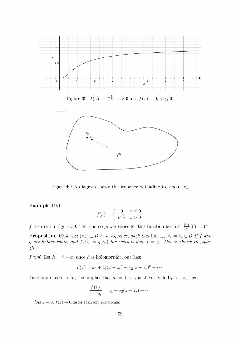
Figure 39: f(x) = e−1x , x > 0 and f(x) = 0, x ≤ 0.
Figure 40: A diagram shown the sequence zi tending to a point z∗.
Example 19.1.
f(x) =
0 x ≤ 0
e−1x x > 0
f is drawn in figure 39. There is no power series for this function because ∂nf∂xn
(0) = 032
Proposition 19.4. Let (zn) ⊂ D be a sequence, such that limn→∞ zn = z∗ ∈ D If f andg are holomorphic, and f(zn) = g(zn) for every n then f = g. This is shown in figure40.
Proof. Let h = f − g, since h is holomorphic, one has:
h(z) = a0 + a1(z − z∗) + a2(z − z∗)2 + · · ·
Take limits as n→∞, this implies that a0 = 0. If you then divide by z − z∗ then:
h(z)
z − z∗= a1 + a2(z − z∗) + · · ·
32As x→ 0, f(x)→ 0 faster than any polynomial
59

If you evaluate at z = zn and take limits as n → ∞ we get a1 = 0. By induction, youthen get ak = 0 ∀k.
Remark 19.4. If (zn) doesn’t converge the above doesn’t hold. e.g. f(x) = sin x, g(x) = 0[(zn) = kπk ∈ Z] e.g. f(x) = sin2 x+cos2 x g(x) = 1 One has sin2 x+cos2 x = 1 ∀x ∈ C.
Theorem 19.5. Let f : C → C be holomorphic, if their exists M such that |f(z)| < M∀z ∈ C then f is constant.
Proof. We have:
f(z) =∞∑n=0
anzn
with
an =1
2πi
∫B(0,R)
f(z)
zn+1dz
|an| =1
2π
∣∣∣∣∫B(0,R)
f(z)
zn+1dz
∣∣∣∣ ≤ 1
2π
∫B(0,R)
∣∣∣∣f(z)
zn+1
∣∣∣∣ dz≤ 1
2π
∫B(0,R)
M
Rn+1dz
|an| ≤1
2π
M
Rn+12πR =
M
Rn
This holds for every R > 0, therefore an = 0 for n ≥ 1. This means that
f(z) =∞∑n=0
anzn = a0
(i.e. f(z) is constant.)
Theorem 19.6. Every non-constant polynomial P on C has at least one root. (∃ z ∈ Cs.t P (z) = 0)
Proof. Suppose f has no root. Then f(z) = 1P (z)
is holomorphic in C. P = a0 + a1 +
· · · + anzn There exists an R > 0 and C > 0 s.t. |P (t)| ≥ C|z|n for |z| > R. Therefore
|f(z)| ≤ 1CRn
for |z| > R. Since P has no root, f has no C pole (i.e. 1/0 is undefined)[3],this means that their exists M s.t |f(z)| < M for |z| < R, by the previous theorem fmust be constant, which implies that P is also constant. If P is a polynomial of degreen and P (a) = 0, then P (z) = (z − a)P (z) where P is a polynomial of degree n− 1.
20 Real Sums
The aim is to find the solution of:∞∑
k=−∞
(20.1)
60

Figure 41: A diagram of the box γN
61

Idea: calculate ∫γN
f(z)cos(πz)
sin(πz)dz
f is holomorphic except at z1, z2, . . . , zM .∫γN
f(z)cos(πz)
sin(πz)dz (20.2)
=︸︷︷︸CIF
M∑k=1
∫δB(zN ,ε)
· · ·+N∑
k=−N
2πif(k)
π
This allows us to compute∑N
k=−N f(k).
Remark 20.1 (Details).
sin(πz) =eiπz − e−iπz
2i= 0
⇒ eiπz − e−iπz ⇒ z ∈ ZUsing:
sin(z) = z − z3
3!+z5
5!− · · ·
As we know that sin(a+ b) = sin a cos b+ cos a sin b
sin(πz) = sin(π(z − k) + πk
)= sin
(π(z − k)
)cos πk + cos
(π(z − k)
)sin(πk)︸ ︷︷ ︸
=0
= π(z − k)
(1− π2(z − k)2
3!+ ·)
︸ ︷︷ ︸=g(z)→z as z→k
cos(πk)
⇒∫δB(k,ε)
f(z)cos(πz)
sin(πz)=
∫1
z − kf(z)
cos(πk)
πg(z) cos(pik)
=︸︷︷︸CIF
2πif(k)cos(πk)
π − cos(πk)= 2if(k)
Example 20.1.
f(z) =1
z2 + 1=
1
(z − i)(z + i)
At i :
∫δB(i,ε)
f(z)cos(πz)
sin(πz)=︸︷︷︸CIF
2πi1
i+ i
cos(πi)
sin(πi)= π
cos(πi)
sin(πi)
At − i : 2πi1
−i− icos(−πi)sin(−πi)
= πcos(πi)
sin(πi)
, cos(πz)sin(πz)
has poles at 1π(z−k)
for z ∈ Z. The integral along the box γN (as shown if figure
41) as N →∞.∣∣∣∣∫γN
f(z)cos(πz)
sin(πz)dz
∣∣∣∣ ≤ maxz∈γN|· · · | · (Length of γN) ≤ C
N2· 4(2N + 1)→ 0
62

With N →∞
0 = 2πcos(πi)
sin(πi)+ 2i
∞∑k=−∞
1
k2 + 1
⇒∞∑
k=−∞
1
k2 + 1=−πi
cos(πi)
sin(πi)
⇒∞∑
k=−∞
1
k2 + 1=π cosh π
sinhπ= π tanh(π) ≈ 3.15
References
[1] Cauchy Schwarz inequality on Wikipediahttp://en.wikipedia.org/wiki/Cauchy-Schwarz_inequality
[2] Kissing Number Problemwww.lix.polytechnique.fr/~liberti/kissing-ctw.ps.gz
[3] Pole (Complex Analysis)http://en.wikipedia.org/wiki/Pole_(complex_analysis)
63