IIIIIndicndicndicndicndicatatatatators of Cors of Cors of Cors of Cors of Climlimlimlimlimatatatatate Ce Ce Ce Ce Chhhhhananananangggggeeeeein tin tin tin tin thhhhhe Ne Ne Ne Ne Nortortortortorthhhhheasteasteasteasteast

20052005200520052005

CCCCClean Alean Alean Alean Alean Air - Cir - Cir - Cir - Cir - Cool Plool Plool Plool Plool Planeaneaneaneanetttttandandandandand

CCCCCameameameameamerrrrrooooon Pn Pn Pn Pn P..... W W W W WaaaaakkkkkeeeeeTTTTThhhhhe Ce Ce Ce Ce Climlimlimlimlimatatatatate Ce Ce Ce Ce Chhhhhanananananggggge Re Re Re Re Researesearesearesearesearccccch Ch Ch Ch Ch Cenenenenenttttteeeeerrrrr,,,,,

UUUUUnnnnniviviviviveeeeersrsrsrsrsity of Nity of Nity of Nity of Nity of Neeeeew Hw Hw Hw Hw Hamamamamampspspspspshhhhhiririririreeeee

IIIIIndicndicndicndicndicatatatatators of Cors of Cors of Cors of Cors of Climlimlimlimlimatatatatate Ce Ce Ce Ce Chhhhhananananangggggeeeeein tin tin tin tin thhhhhe Ne Ne Ne Ne Nortortortortorthhhhheasteasteasteasteast

20052005200520052005

CCCCClean Alean Alean Alean Alean Air - Cir - Cir - Cir - Cir - Cool Plool Plool Plool Plool Planeaneaneaneanetttttandandandandand

CCCCCameameameameamerrrrrooooon Pn Pn Pn Pn P..... W W W W WaaaaakkkkkeeeeeTTTTThhhhhe Ce Ce Ce Ce Climlimlimlimlimatatatatate Ce Ce Ce Ce Chhhhhanananananggggge Re Re Re Re Researesearesearesearesearccccch Ch Ch Ch Ch Cenenenenenttttteeeeerrrrr,,,,,

UUUUUnnnnniviviviviveeeeersrsrsrsrsity of Nity of Nity of Nity of Nity of Neeeeew Hw Hw Hw Hw Hamamamamampspspspspshhhhhiririririreeeee

Copyright 2005 ©©©©© Clean Air - Cool Planet

AAAAAccccckkkkknononononowlwlwlwlwledededededgggggemenemenemenemenementttttsssss

J. Bloomfield, S. Droege, L. Goss, S. Hamburg, B. Harrington, J. Kelley, K. Kimball, S. Moser, B. Rock,C. Rogers, H. Walker, W. White and N. Willard all contributed significantly to the concept for this projectthrough their participation in a Northeast climate indicators workshop convened by Clean Air-Cool Planetin Portsmouth, NH in January 2001. Dr. Tim Sparks of the Center for Ecology and Hydrology at MonksWood, England, and a founder of the UK Phenology Network helped to plan that workshop and providedthe inspiration for this report.

We would like to acknowledge the hard work of UNH graduate student Adam Wilson in assembling andanalyzing the data for many of these indicators; the work of Professor David Wolfe in the HorticultureDepartment at Cornell University for authoring the section on phenology (bloom dates), along with hiscollaborators A. Lakso and Y. Otsuki at Cornell University and M. Schwartz at University of Wisconsin-Milwaukee; and UNH graduate student Gerry Hornok for data analysis and preparation of select graphics.T. Huntington and B. Keim also provided material incorporated into this report; we are indebted to K.Colburn at NESCAUM, N. Anderson at the Maine Lung Association, and others for their careful review.Most of the photographs are by Jerry and Marcy Monkman at EcoPhotography.

A downloadable Adobe Acrobat file is available at http://cleanair-coolplanet.org/information/pdf/indicators.pdf

TTTTTaaaaablblblblble of Ce of Ce of Ce of Ce of Cooooonnnnntttttenenenenentttttsssss

Introduction ................................................................................ 1

Average Annual Temperature..................................................2

Length of Growing Season .....................................................4

Bloom Dates ...................................................................................6

Timing of High Spring Flow and River Ice-Out...............10

Lake Ice-In and -Out Dates ......................................................13

Precipitation ...............................................................................16

Intense Precipitation Events ..............................................18

Sea Level Rise .............................................................................20

Sea Surface Temperature ......................................................22

Snowfall .......................................................................................24

Days with Snow on the Ground ..........................................26

Summary.....................................................................................................................28

References...............................................................................................................30

IIIIInnnnntttttrrrrroduoduoduoduoductctctctctioioioioionnnnn

1 .1 .1 .1 .1 .

Climate changes. It always has and always will. What is unique in modern times is thathuman activities are now a significant factor causing climate to change. This is evident inthe recent rise in key greenhouse gases, such as carbon dioxide (CO2), in the atmosphere,and in the recent increase in global temperatures in the lower atmosphere and in thesurface ocean.

The evidence presented in this report clearly illustrates that climate in New England isalso changing. Over the past 100 years, and especially the last 30 years, all of the climatechange indicators for the region reveal a warming trend. While at this point we cannotprove conclusively that this regionl warming is due to human actions, the warming is fullyconsistent with what we would expect from global warming caused by increasinggreenhouse gas concentrations.

There is no question that human induced climate change is a phenomenon thathumans will have to deal with in the coming decades. The good news is that, because weare the primary source of pollution that is likely causing our atmosphere and oceans towarm, we can also do something about it by changing specific policies and behaviors.

It is our hope that by presenting this information in a succinct format, more peoplewill understand the nature and scope of the problem and, therefore, be willing to make thechanges necessary.

For more information about the science of global warming and the practicality ofsolutions, please visit the Clean Air – Cool Planet (www.cleanair-coolplanet.org) and theUniversity of New Hampshire – Climate Education Initiative (www.sustainableunh.unh.edu/climate_ed/) web sites.

Adam MarkhamAdam MarkhamAdam MarkhamAdam MarkhamAdam MarkhamEEEEExxxxxecutecutecutecutecut iiiii vvvvve Die Die Die Die Dirrrrr e c te c te c te c te c tooooorrrrr,,,,,CCCCClean Alean Alean Alean Alean Aiiiiir - Cr - Cr - Cr - Cr - Cooooooooool Pll Pll Pll Pll Planeaneaneaneanettttt

CCCCCameameameameamerrrrrooooo n Wn Wn Wn Wn WaaaaakkkkkeeeeeRRRRReseaeseaeseaeseaesearrrrrccccch Ah Ah Ah Ah Associassociassociassociassociattttte Pe Pe Pe Pe Prrrrrooooofffffessoessoessoessoessorrrrr,,,,,University of New HampshireUniversity of New HampshireUniversity of New HampshireUniversity of New HampshireUniversity of New HampshireCCCCC l i ml i ml i ml i ml i maaaaattttt e Ce Ce Ce Ce Chhhhh a na na na na n ggggge Re Re Re Re Reseaeseaeseaeseaesearrrrrccccch Ch Ch Ch Ch Ceeeee nnnnnttttteeeee rrrrr

March, 2005March, 2005March, 2005March, 2005March, 2005

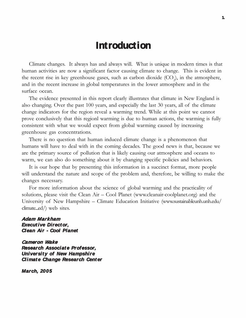
AAAAAvvvvveeeeerrrrragagagagage Ae Ae Ae Ae Annnnnnnnnnuuuuuaaaaal Tl Tl Tl Tl Teeeeemmmmmpepepepeperrrrraturaturaturaturatureeeee1899 t1899 t1899 t1899 t1899 thhhhhrrrrrooooouuuuugggggh 2000h 2000h 2000h 2000h 2000

Indicator OverviewIndicator OverviewIndicator OverviewIndicator OverviewIndicator OverviewTemperature is one of most frequent-

ly used indicators of climate change andhas been recorded at numerous stationsin the Northeast United States since1899. It is possible to analyze the region’schanging climate over the past centurywith this long-term instrumental recordof average monthly temperature.1

RRRRReeeeegggggioioioioionnnnnaaaaal Il Il Il Il ImmmmmpopopopoportrtrtrtrtancancancancanceeeeeWeather in the Northeast is as di-

verse as it is variable. Mark Twain cap-tured the essence of the region’s climatewhen he stated “Yes, one of the bright-est gems in the New England weather isthe dazzling uncertainty of it.” 2 Chang-es in temperature affect numerous as-pects of our daily lives and our region’s economy, including the ski industry, tourism, transportation, agricul-ture, emergency management, health, and fuel consumption for heating and cooling. Temperature is thedeterminant factor in the length of the growing season, it influences the amount of winter snowfall, and thecomfort of a summer afternoon.

The National Oceanographic and Atmospheric Administration’s National Climatic Data Center has main-tained temperature records from various stations across the country. In the Northeast there are 56 stations thathave been continuously operating since 1899, providing the best record of temperature variations for the region.

SSSSSeeeeensnsnsnsnsiiiiitttttiiiiivvvvviiiiittttty ty ty ty ty to Co Co Co Co Climlimlimlimlimaaaaattttte and Oe and Oe and Oe and Oe and Ottttthhhhheeeeer Fr Fr Fr Fr FactactactactactooooorrrrrsssssGlobal surface temperatures reflect the interaction of several aspects of Earth’s climate system, includ-

ing the amount of incoming sunlight, volcanic activity, land use changes, the ability of the planet to reflectlight, the exchange of energy between the ocean and the atmosphere, and the concentration of greenhousegases and other pollutants. Since the 1860s, average global temperature has increased by about 1.1o

F, likely

due to increasing greenhouse gases from human activities.3On a regional scale, the average temperature of the Northeast is sensitive to the same global influences,

but also local aspects of the climatic system, including the locations of weather systems, storm tracks,fluctuations in the jet stream, topography, and changing ocean currents and sea surface temperatures.

IIIIIndicndicndicndicndicaaaaatttttooooor Tr Tr Tr Tr TrrrrreeeeendndndndndAnnual average temperature for the Northeast shows considerable variability on annual and longer time

scales (Figure 1). For example, note the cooler years in 1904, 1917, and 1926 and the relatively warm yearsin 1949, 1953, 1990, and 1998. Extended warm periods are also evident, such as the early 1930s and the late

2 .2 .2 .2 .2 .

Figure 1: Average annual temperature for the Northeast from 1899 through2000. This time-series is an areally weighted average of temperaturerecords from 56 stations in the region.

1940s. Cool periods occurredat the beginning of the centu-ry and the late 1960s.

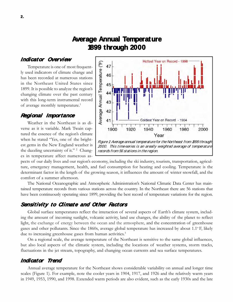
There is also a trend to-wards warmer temperaturesover the period of record.Based on the linear trend, theNortheast’s average annualtemperature has increased byabout 1.8o F since 1899. The1990s were the warmest de-cade on record. Over the last30 years, annual average tem-peratures have increased 1.4o

F. The meteorological stationdata allows for an investiga-tion of temperature change ona finer scale. As illustrated onthe map of the Northeast, allof the stations but oneshowed an increase in temper-ature (Figure 2). Note that thecoastal regions of Massachu-setts, New Jersey, New York,Connecticut and Maine haveall warmed more than the

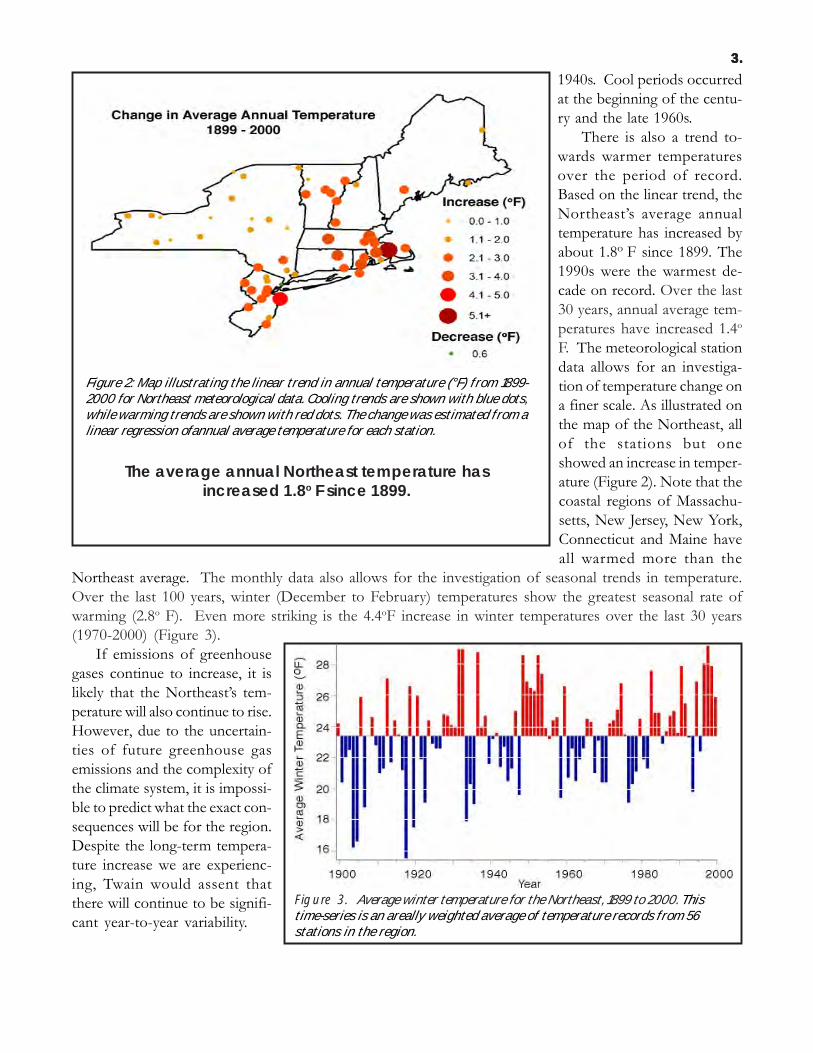
Northeast average. The monthly data also allows for the investigation of seasonal trends in temperature.Over the last 100 years, winter (December to February) temperatures show the greatest seasonal rate ofwarming (2.8o F). Even more striking is the 4.4oF increase in winter temperatures over the last 30 years(1970-2000) (Figure 3).

If emissions of greenhousegases continue to increase, it islikely that the Northeast’s tem-perature will also continue to rise.However, due to the uncertain-ties of future greenhouse gasemissions and the complexity ofthe climate system, it is impossi-ble to predict what the exact con-sequences will be for the region.Despite the long-term tempera-ture increase we are experienc-ing, Twain would assent thatthere will continue to be signifi-cant year-to-year variability.

3 .3 .3 .3 .3 .

Figure 3. Average winter temperature for the Northeast, 1899 to 2000. Thistime-series is an areally weighted average of temperature records from 56stations in the region.

Figure 2: Map illustrating the linear trend in annual temperature (°F) from 1899-2000 for Northeast meteorological data. Cooling trends are shown with blue dots,while warming trends are shown with red dots. The change was estimated from alinear regression ofannual average temperature for each station.

The average annual Northeast temperature hasincreased 1.8o F since 1899.

Length of Growing SeasonLength of Growing SeasonLength of Growing SeasonLength of Growing SeasonLength of Growing Season1874 - 20011874 - 20011874 - 20011874 - 20011874 - 2001

Indicator OverviewIndicator OverviewIndicator OverviewIndicator OverviewIndicator OverviewLength of the growing season is de-

fined as the number of days between thelast frost of spring and the first frost ofwinter. This period is called the growingseason because it roughly marks the peri-od during which plants, especially agricul-tural crops, grow most successfully.

RRRRReeeeegggggioioioioionnnnnaaaaal Il Il Il Il ImmmmmpopopopoportrtrtrtrtancancancancanceeeeeThe length of the growing season is

important to any outdoor activity. Whilefreezing temperatures affect all commer-cial, agricultural, industrial, recreation-al, and ecological systems, the humansystem most sensitive to changes in thelength of the growing season is agricul-ture.4

An early fall frost may lead to crop failure and economic misfortune to the farmer. Earlier starts to thegrowing season may provide an opportunity to diversify crops, or to produce two or more harvests from thesame plot. However, the majority of the Northeast’s most competitive crops are “cool-season” crops. While

it might seem that a successful response to a shorter growing season would befor farmers to switch to alternative warm-season crops, they would then havenew competitors who might have advantages such as better soils and a longergrowing season.5 In either case, the length of the growing season is very im-portant to successful agriculture in this region.

In addition, the length of the growing season is a defining characteristicof different ecosystems.6 It is possible that a significant change in the lengthof the growing season could alter the ecology of the Northeast landscape.

SSSSSeeeeensnsnsnsnsiiiiitttttiiiiivvvvviiiiittttty ty ty ty ty to Co Co Co Co Climlimlimlimlimaaaaattttte and Oe and Oe and Oe and Oe and Ottttthhhhheeeeer Fr Fr Fr Fr FactactactactactooooorrrrrsssssGrowing season length is an event-driven phenomenon. An increase in theaverage temperature for a region does not necessarily imply an increase in thegrowing season, and vice versa. As the growing season is defined by the lastfrost of the spring and the first of the fall, it is solely dependent on specificcold weather events, rather than monthly or annual averages.

There are two types of frost events, radiation and advective frosts.7 Energy absorbed from the sun byday radiates upward to space by night, causing the air near the surface to cool. On most nights there isenough wind to mix the warmer, upper air with the surface air and keep surface temperatures relativelywarm. However, on calm, dry nights, the air near the surface radiates heat upward without mixing with it,

4 .4 .4 .4 .4 .

-20

-10

0

10

20

30

1900 1920 1940 1960 1980 2000

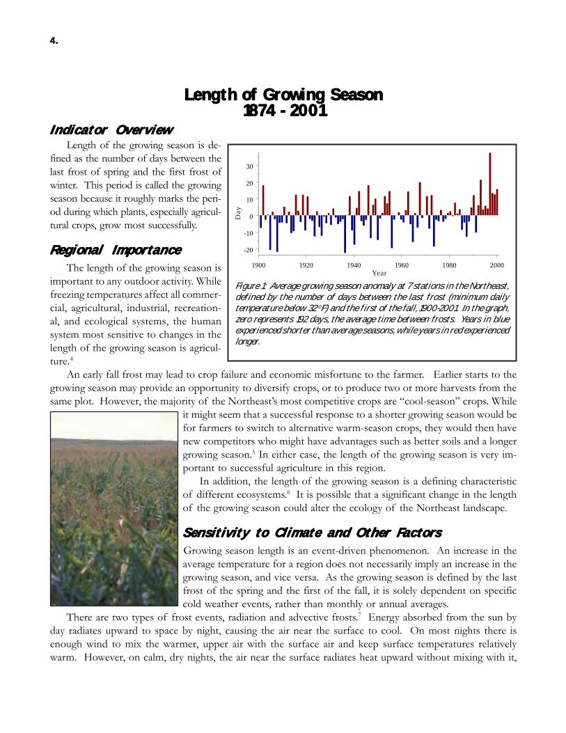
Figure 1: Average growing season anomaly at 7 stations in the Northeast,defined by the number of days between the last frost (minimum dailytemperature below 32 oF) and the first of the fall, 1900-2001. In the graph,zero represents 192 days, the average time between frosts. Years in blueexperienced shorter than average seasons, while years in red experiencedlonger.

Day

Year

creating very cold air at the surface— a radiation frost. This type of frostgenerally impacts relatively small geo-graphic regions and occurs mostly invalleys.

Advective frosts are caused by acold, polar airmass moving into theregion. This type of frost is associat-ed with strong winds and a well-mixedatmosphere and tends to affect largegeographic areas. The most damag-ing frosts are combinations of thesetwo types. First the polar airmassmoves through and cools down a re-gion, after which the winds slowdown and can create ideal conditionsfor a radiative frost.

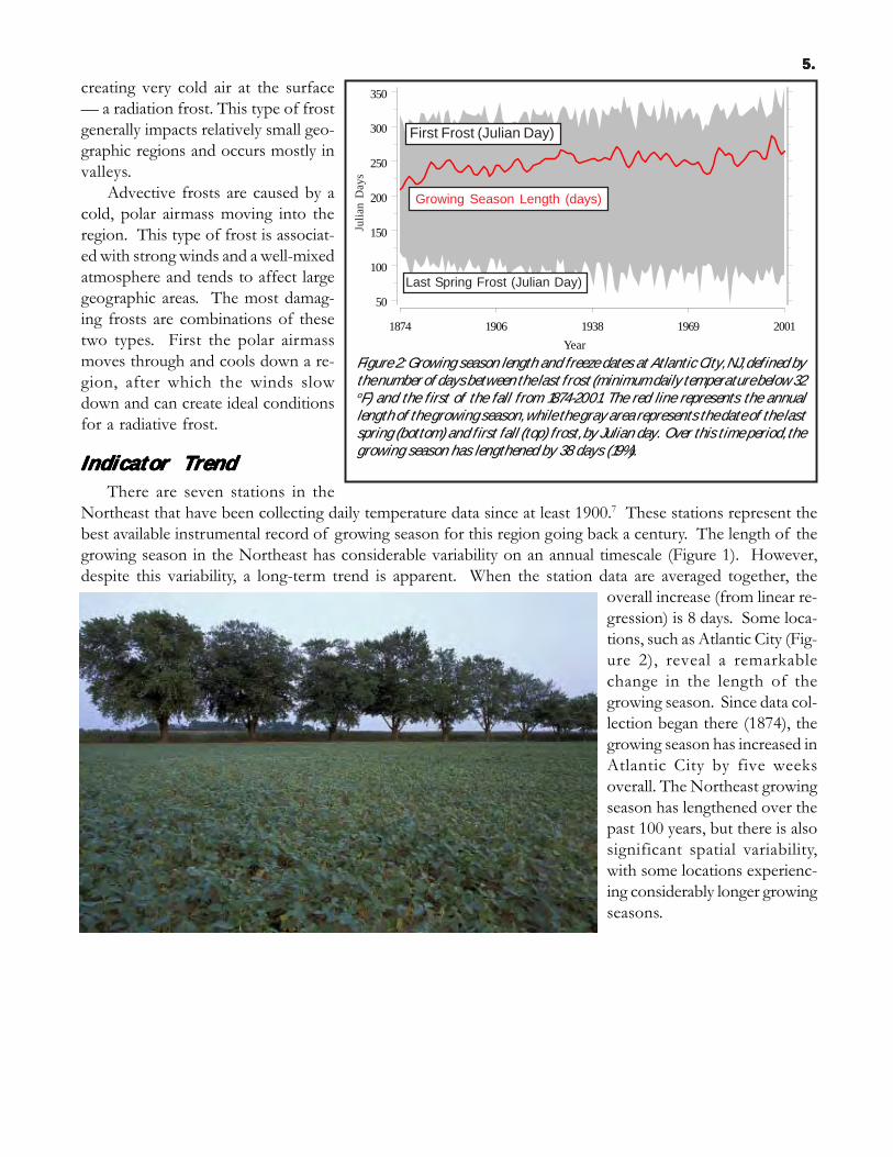
IIIIIndicndicndicndicndicaaaaatttttooooor Tr Tr Tr Tr TrrrrreeeeendndndndndThere are seven stations in the

Northeast that have been collecting daily temperature data since at least 1900.7 These stations represent thebest available instrumental record of growing season for this region going back a century. The length of thegrowing season in the Northeast has considerable variability on an annual timescale (Figure 1). However,despite this variability, a long-term trend is apparent. When the station data are averaged together, the

overall increase (from linear re-gression) is 8 days. Some loca-tions, such as Atlantic City (Fig-ure 2), reveal a remarkablechange in the length of thegrowing season. Since data col-lection began there (1874), thegrowing season has increased inAtlantic City by five weeksoverall. The Northeast growingseason has lengthened over thepast 100 years, but there is alsosignificant spatial variability,with some locations experienc-ing considerably longer growingseasons.

5 .5 .5 .5 .5 .

1874 1906 1938 1969 2001Year

50

100

150

200

250

300

350

Last Spring Frost (julian day)

Growing Season Length (days)

First Fall Frost (julian day)

Last Spring Frost (Julian Day)

First Frost (Julian Day)

Growing Season Length (days)

Figure 2: Growing season length and freeze dates at Atlantic City, NJ, defined bythe number of days between the last frost (minimum daily temperature below 32oF) and the first of the fall from 1874-2001. The red line represents the annuallength of the growing season, while the gray area represents the date of the lastspring (bottom) and first fall (top) frost, by Julian day. Over this time period, thegrowing season has lengthened by 38 days (19%).

Julia

n D

ays

BBBBBloolooloolooloom Dm Dm Dm Dm Datatatatates fes fes fes fes for Lilor Lilor Lilor Lilor Lilacsacsacsacsacs,,,,, A A A A Apppppplesplesplesplesples,,,,, and Gr and Gr and Gr and Gr and Graaaaapespespespespes

Indicator OverviewIndicator OverviewIndicator OverviewIndicator OverviewIndicator OverviewAs evidence of climate change mounts, scientists have begun to search for signs of biological or ecological

responses to this change. A shift in seasonal events in the life of plants and animals, such as flower bloom,spring arrival of migrating birds and insects, etc., are potential “bioindicators” of climate change.

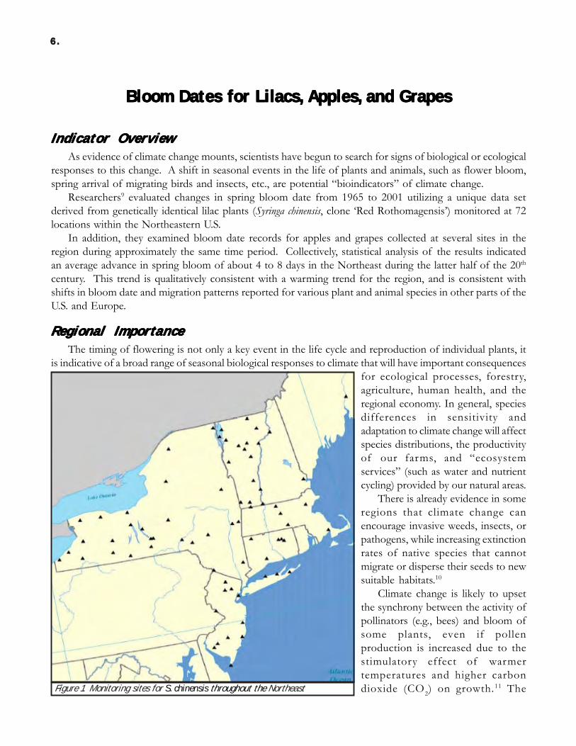
Researchers9 evaluated changes in spring bloom date from 1965 to 2001 utilizing a unique data setderived from genetically identical lilac plants (Syringa chinensis, clone ‘Red Rothomagensis’) monitored at 72locations within the Northeastern U.S.

In addition, they examined bloom date records for apples and grapes collected at several sites in theregion during approximately the same time period. Collectively, statistical analysis of the results indicatedan average advance in spring bloom of about 4 to 8 days in the Northeast during the latter half of the 20th

century. This trend is qualitatively consistent with a warming trend for the region, and is consistent withshifts in bloom date and migration patterns reported for various plant and animal species in other parts of theU.S. and Europe.

RRRRReeeeegggggioioioioionnnnnaaaaal Il Il Il Il ImmmmmpopopopoportrtrtrtrtancancancancanceeeeeThe timing of flowering is not only a key event in the life cycle and reproduction of individual plants, it

is indicative of a broad range of seasonal biological responses to climate that will have important consequencesfor ecological processes, forestry,agriculture, human health, and theregional economy. In general, speciesdifferences in sensitivity andadaptation to climate change will affectspecies distributions, the productivityof our farms, and “ecosystemservices” (such as water and nutrientcycling) provided by our natural areas.

There is already evidence in someregions that climate change canencourage invasive weeds, insects, orpathogens, while increasing extinctionrates of native species that cannotmigrate or disperse their seeds to newsuitable habitats.10

Climate change is likely to upsetthe synchrony between the activity ofpollinators (e.g., bees) and bloom ofsome plants, even if pollenproduction is increased due to thestimulatory effect of warmertemperatures and higher carbondioxide (CO2) on growth.11 The

6 .6 .6 .6 .6 .

Figure 1. Monitoring sites for S. chinensis throughout the Northeast

pollen-allergy season is likely to arrive earlier in the spring and could be more severe in a warmer high-CO2world.12 Finally, flowering time and fruit set are driving factors in the food web upon which humans alldepend. Pollen, nectar, fruit, or seeds are important resources for many animals, including farmers, humanconsumers of farm products, and those involved in the agricultural economy of the region.

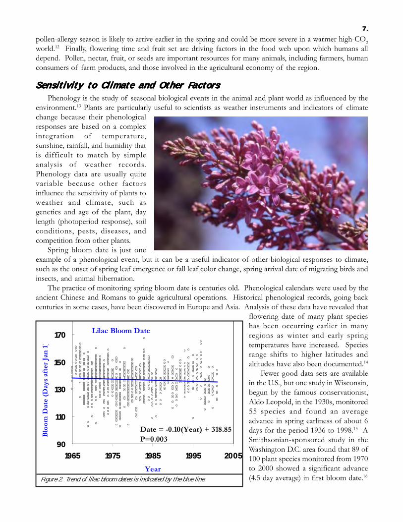
SSSSSeeeeensnsnsnsnsiiiiitttttiiiiivvvvviiiiittttty ty ty ty ty to Co Co Co Co Climlimlimlimlimaaaaattttte and Oe and Oe and Oe and Oe and Ottttthhhhheeeeer Fr Fr Fr Fr FactactactactactooooorrrrrsssssPhenology is the study of seasonal biological events in the animal and plant world as influenced by the

environment.13 Plants are particularly useful to scientists as weather instruments and indicators of climatechange because their phenologicalresponses are based on a complexintegration of temperature,sunshine, rainfall, and humidity thatis difficult to match by simpleanalysis of weather records.Phenology data are usually quitevariable because other factorsinfluence the sensitivity of plants toweather and climate, such asgenetics and age of the plant, daylength (photoperiod response), soilconditions, pests, diseases, andcompetition from other plants.

Spring bloom date is just oneexample of a phenological event, but it can be a useful indicator of other biological responses to climate,such as the onset of spring leaf emergence or fall leaf color change, spring arrival date of migrating birds andinsects, and animal hibernation.

The practice of monitoring spring bloom date is centuries old. Phenological calendars were used by theancient Chinese and Romans to guide agricultural operations. Historical phenological records, going backcenturies in some cases, have been discovered in Europe and Asia. Analysis of these data have revealed that

flowering date of many plant specieshas been occurring earlier in manyregions as winter and early springtemperatures have increased. Speciesrange shifts to higher latitudes andaltitudes have also been documented.14

Fewer good data sets are availablein the U.S., but one study in Wisconsin,begun by the famous conservationist,Aldo Leopold, in the 1930s, monitored55 species and found an averageadvance in spring earliness of about 6days for the period 1936 to 1998.15 ASmithsonian-sponsored study in theWashington D.C. area found that 89 of100 plant species monitored from 1970to 2000 showed a significant advance(4.5 day average) in first bloom date.16

7 .7 .7 .7 .7 .

Lilac Bloom Date

Date = -0.10(Year) + 318.85P=0.003

90

110

130

150

170

1965 1975 1985 1995 2005

Year

Blo

om D

ate

(Day

s af

ter

Jan

1)

Figure 2. Trend of lilac bloom dates is indicated by the blue line.

8 .8 .8 .8 .8 .

The results presented here focusspecifically on the northeastern U.S., whereaverage annual temperatures increased 1.8o F,and winter temperatures (December throughFebruary) increased 2.8o F from 1899 to 2000.Records were evaluated from 72 locations inthis region (see map, Fig. 1) where geneticallyidentical lilac plants (S. chinensis, clone ‘RedRothomagensis’) were planted and monitoredfor first flower (bloom) date during the period1965 to 2001. Not all sites were establishedin the same year, and most sites were missingsome years of record. On average, the sitesused had 21 years of record. These plantingswere originally established by a U.S. Department of Agriculture project17 for the purpose of using phenologicalinformation to optimize farming practices (e.g., seeding date and pest control), and predict yield potential(crop “futures”) for several economically important crops.

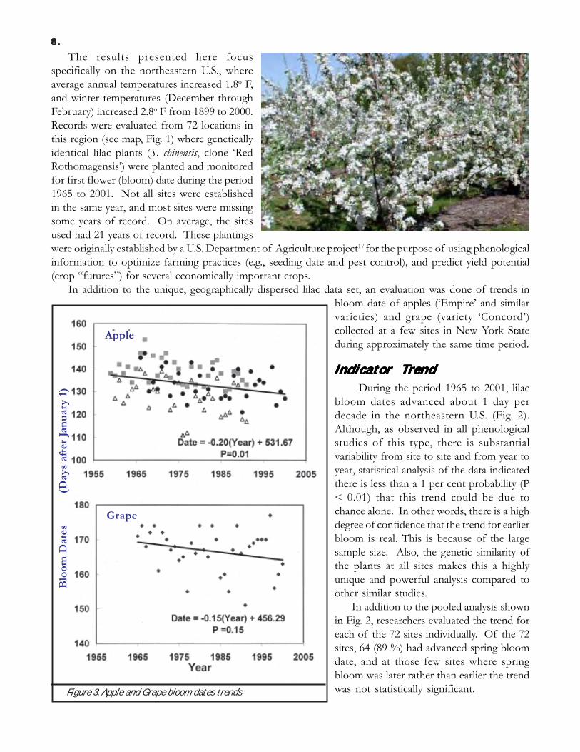
In addition to the unique, geographically dispersed lilac data set, an evaluation was done of trends inbloom date of apples (‘Empire’ and similarvarieties) and grape (variety ‘Concord’)collected at a few sites in New York Stateduring approximately the same time period.

IIIIIndicndicndicndicndicaaaaatttttooooor Tr Tr Tr Tr TrrrrreeeeendndndndndDuring the period 1965 to 2001, lilac

bloom dates advanced about 1 day perdecade in the northeastern U.S. (Fig. 2).Although, as observed in all phenologicalstudies of this type, there is substantialvariability from site to site and from year toyear, statistical analysis of the data indicatedthere is less than a 1 per cent probability (P< 0.01) that this trend could be due tochance alone. In other words, there is a highdegree of confidence that the trend for earlierbloom is real. This is because of the largesample size. Also, the genetic similarity ofthe plants at all sites makes this a highlyunique and powerful analysis compared toother similar studies.

In addition to the pooled analysis shownin Fig. 2, researchers evaluated the trend foreach of the 72 sites individually. Of the 72sites, 64 (89 %) had advanced spring bloomdate, and at those few sites where springbloom was later rather than earlier the trendwas not statistically significant.Figure 3. Apple and Grape bloom dates trends

Apple

Grape

Blo

om D

ates

(D

ays

afte

r Ja

nu

ary

1)

9 .9 .9 .9 .9 .

Analysis of the more geographically limited apple and grape datasets (Fig. 3) suggests a slightly more rapid advance in spring bloom(about 2 days per decade, or 8 days since the 1960s) for these speciescompared to lilac.

The implications of earlier bloom for agricultural crops will dependon many factors. In some cases, it may translate in a straightforwardfashion to earlier yields. This will benefit farmers who receive higherprices for earlier production, but could have a negative effect if there isincreased competition from farmers in other regions earlier in the season.

Earlier bloom could potentially reduce yields if spring temperaturesbecome more variable as the climate changes and an early bloomincreases the risk of frost damage to flowers and developing fruit. Arecent analysis of historical apple yields in the New York State region18

found that warmer temperatures during the January 1 to bud breakperiod was correlated with lower, not higher yields.

Collectively, analyses for the northeastern U.S. indicate that, onaverage, lilacs are blooming about four days earlier, and apple and grapesare blooming about eight days earlier than they were half a century ago.The magnitude of this climate impact on woody perennials in theNortheast is similar to that reported for bloom of other plant species,

and for bird and insect spring migration arrivals, by researchers in other parts of the U.S. and Europe (references:see footnotes 9-11). Results are also qualitatively in agreement with reports of earlier spring “green wave”advancement in the northern hemisphere based on satellite imagery of vegetative cover.19

This and other recent phenology studies have relied on historical records that were initially maintainedfor purposes other than examination of climate change. Given the importance of reliable data on ecologicalresponses to climate change for policy-makers, strengthening the existing regional and global phenologymonitoring networks20 should be a high priority in the future.

TTTTTimimimimiminininining of Hg of Hg of Hg of Hg of Higigigigigh Sh Sh Sh Sh Sppppprrrrrinininining Fg Fg Fg Fg Flololololowwwwwand River Ice-Outand River Ice-Outand River Ice-Outand River Ice-Outand River Ice-Out

Indicator OverviewIndicator OverviewIndicator OverviewIndicator OverviewIndicator OverviewMeasurements associated with river discharge make it possible to rigorously and consistently record both

the timing of high spring flow and the dates of ice-affected flow across the New England region. Both ofthese variables have been collected by the U.S. Geological Survey using consistent methods for many yearson a substantial number of rivers that are free from any significant flow regulation by human activities.

The date marking the point where 50% of the water flow during the period January 1 to May 31 hasoccurred significantly earlier at most of the sites studied for periods ranging from 50 to 95 years through theyear 2000. The date in the Spring when the ice on rivers broke up (ice-out date) has also occurred earlier andthe total number of ice-affected flow days during the winter has decreased on most of the rivers studied.

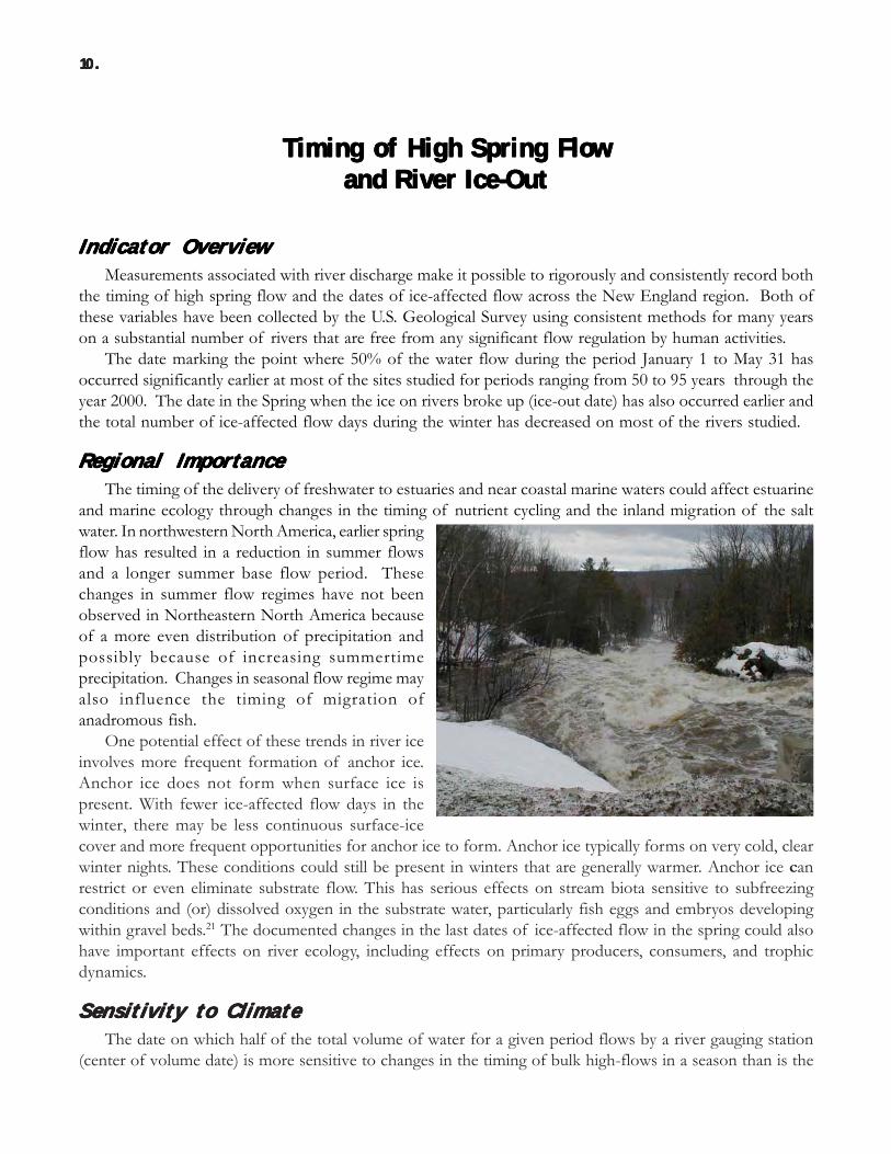
RRRRReeeeegggggioioioioionnnnnaaaaal Il Il Il Il ImmmmmpopopopoportrtrtrtrtancancancancanceeeeeThe timing of the delivery of freshwater to estuaries and near coastal marine waters could affect estuarine

and marine ecology through changes in the timing of nutrient cycling and the inland migration of the saltwater. In northwestern North America, earlier springflow has resulted in a reduction in summer flowsand a longer summer base flow period. Thesechanges in summer flow regimes have not beenobserved in Northeastern North America becauseof a more even distribution of precipitation andpossibly because of increasing summertimeprecipitation. Changes in seasonal flow regime mayalso influence the timing of migration ofanadromous fish.

One potential effect of these trends in river iceinvolves more frequent formation of anchor ice.Anchor ice does not form when surface ice ispresent. With fewer ice-affected flow days in thewinter, there may be less continuous surface-icecover and more frequent opportunities for anchor ice to form. Anchor ice typically forms on very cold, clearwinter nights. These conditions could still be present in winters that are generally warmer. Anchor ice canrestrict or even eliminate substrate flow. This has serious effects on stream biota sensitive to subfreezingconditions and (or) dissolved oxygen in the substrate water, particularly fish eggs and embryos developingwithin gravel beds.21 The documented changes in the last dates of ice-affected flow in the spring could alsohave important effects on river ecology, including effects on primary producers, consumers, and trophicdynamics.

Sensitivity to ClimateSensitivity to ClimateSensitivity to ClimateSensitivity to ClimateSensitivity to ClimateThe date on which half of the total volume of water for a given period flows by a river gauging station

(center of volume date) is more sensitive to changes in the timing of bulk high-flows in a season than is the

10.10.10.10.10.

date of peak flow. This center-of-volumedate is a more robust indicator of seasonalflow timing, since the peak flow date canoccur before or after the bulk of seasonalflows in response to a single storm. Climatewarming results in earlier winter/springseasonal center-of-volume dates because ofan increased ratio of rainfall to snowfall andan earlier snowmelt.

The presence of ice in a river channelaffects the relation between river height andflow; therefore, the presence of ice in rivershas been historically determined andrecorded so that discharge records can beadjusted for the presence of ice. Theformation of ice in river channels is asensitive climate indicator that affects theriver height/flow relation by causingbackwater (a higher-than-normal riverheight for a given flow). This backwater

varies with the quantity and nature of the ice, as well as with the flow. Backwater at a gauging station can becaused by anchor ice or by surface ice. The presence of river ice is readily detected because it results insignature anomalies in the temporal pattern of river stage.

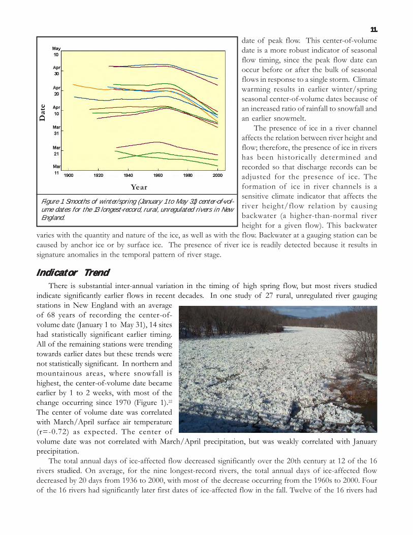
IIIIIndicndicndicndicndicaaaaatttttooooor Tr Tr Tr Tr TrrrrreeeeendndndndndThere is substantial inter-annual variation in the timing of high spring flow, but most rivers studied

indicate significantly earlier flows in recent decades. In one study of 27 rural, unregulated river gaugingstations in New England with an averageof 68 years of recording the center-of-volume date (January 1 to May 31), 14 siteshad statistically significant earlier timing.All of the remaining stations were trendingtowards earlier dates but these trends werenot statistically significant. In northern andmountainous areas, where snowfall ishighest, the center-of-volume date becameearlier by 1 to 2 weeks, with most of thechange occurring since 1970 (Figure 1).22

The center of volume date was correlatedwith March/April surface air temperature(r=-0.72) as expected. The center ofvolume date was not correlated with March/April precipitation, but was weakly correlated with Januaryprecipitation.

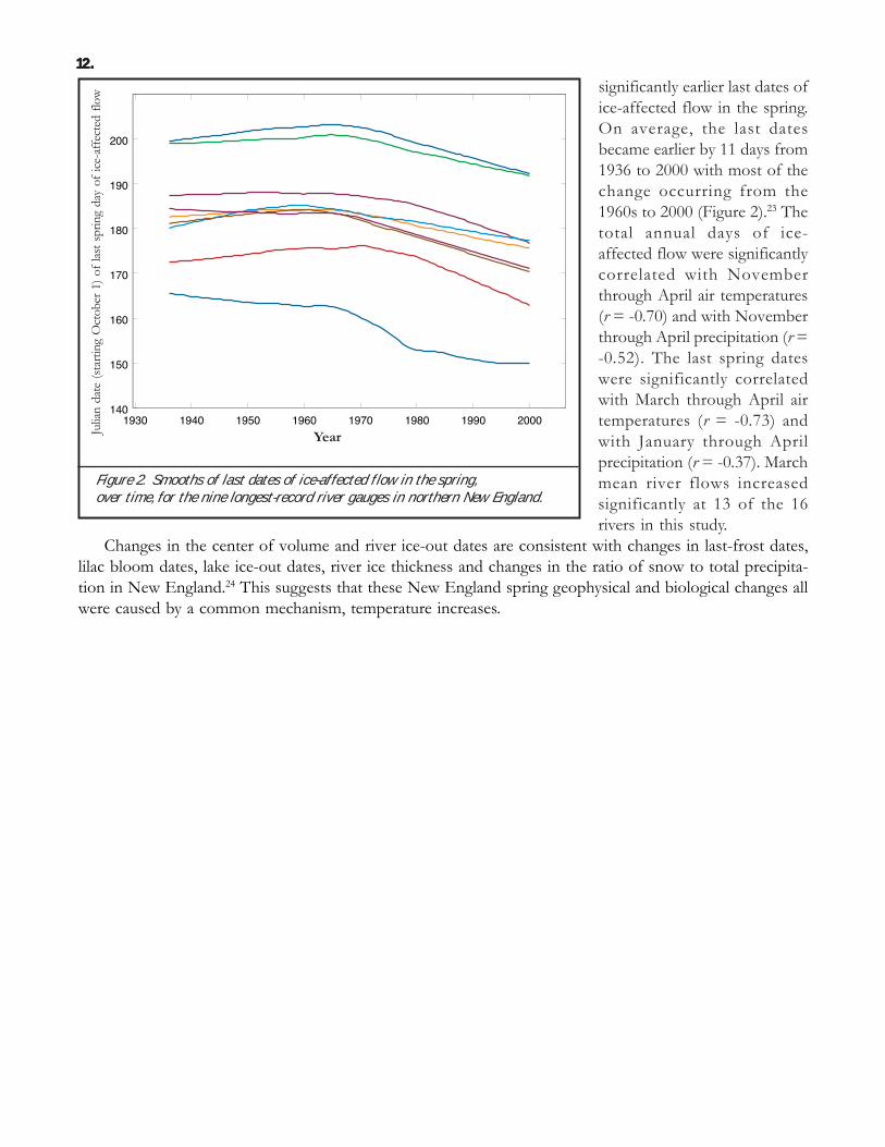
The total annual days of ice-affected flow decreased significantly over the 20th century at 12 of the 16rivers studied. On average, for the nine longest-record rivers, the total annual days of ice-affected flowdecreased by 20 days from 1936 to 2000, with most of the decrease occurring from the 1960s to 2000. Fourof the 16 rivers had significantly later first dates of ice-affected flow in the fall. Twelve of the 16 rivers had

1 1 .1 1 .1 1 .1 1 .1 1 .

Figure 1. Smooths of winter/spring (January 1 to May 31) center-of-vol-ume dates for the 13 longest-record, rural, unregulated rivers in NewEngland.

Year

Dat

e

12 .12 .12 .12 .12 .

significantly earlier last dates ofice-affected flow in the spring.On average, the last datesbecame earlier by 11 days from1936 to 2000 with most of thechange occurring from the1960s to 2000 (Figure 2).23 Thetotal annual days of ice-affected flow were significantlycorrelated with Novemberthrough April air temperatures(r = -0.70) and with Novemberthrough April precipitation (r =-0.52). The last spring dateswere significantly correlatedwith March through April airtemperatures (r = -0.73) andwith January through Aprilprecipitation (r = -0.37). Marchmean river flows increasedsignificantly at 13 of the 16rivers in this study.

Changes in the center of volume and river ice-out dates are consistent with changes in last-frost dates,lilac bloom dates, lake ice-out dates, river ice thickness and changes in the ratio of snow to total precipita-tion in New England.24 This suggests that these New England spring geophysical and biological changes allwere caused by a common mechanism, temperature increases.

Julia

n da

te (s

tarti

ng O

ctob

er 1

) of l

ast s

prin

g da

y of

ice-

affe

cted

flow

Year1930 1940 1950 1960 1970 1980 1990 2000

140

150

160

170

180

190

200

Figure 2. Smooths of last dates of ice-affected flow in the spring,over time, for the nine longest-record river gauges in northern New England.

LLLLLaaaaakkkkke Ie Ie Ie Ie Ice-Ice-Ice-Ice-Ice-In and -Out Dn and -Out Dn and -Out Dn and -Out Dn and -Out Datatatatateseseseses1801801801801807 - 20007 - 20007 - 20007 - 20007 - 2000

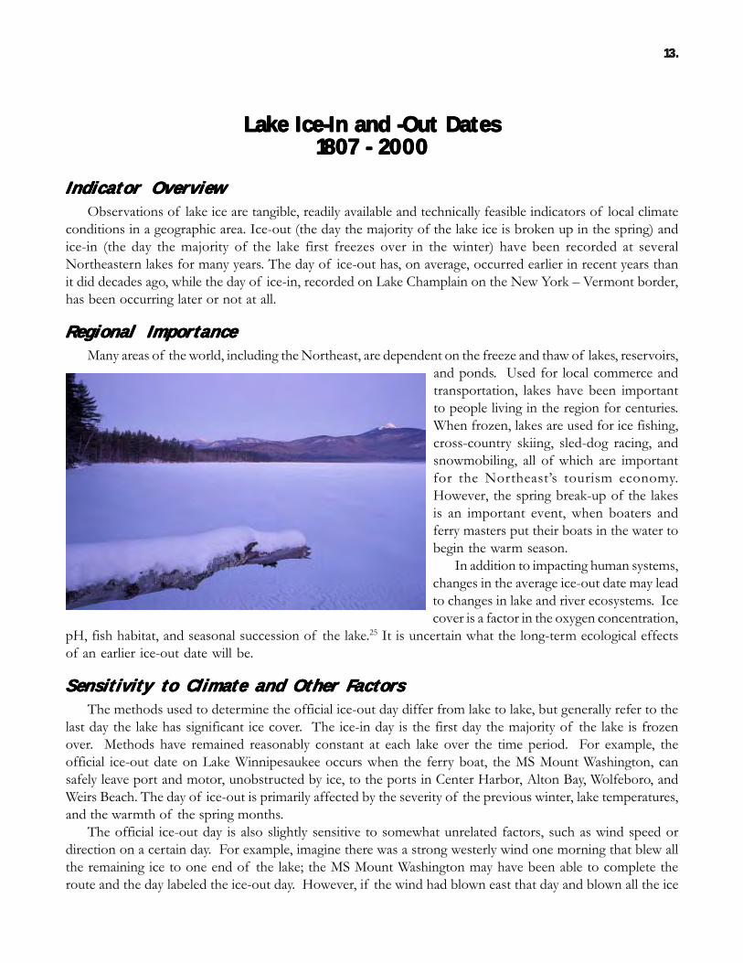
Indicator OverviewIndicator OverviewIndicator OverviewIndicator OverviewIndicator OverviewObservations of lake ice are tangible, readily available and technically feasible indicators of local climate

conditions in a geographic area. Ice-out (the day the majority of the lake ice is broken up in the spring) andice-in (the day the majority of the lake first freezes over in the winter) have been recorded at severalNortheastern lakes for many years. The day of ice-out has, on average, occurred earlier in recent years thanit did decades ago, while the day of ice-in, recorded on Lake Champlain on the New York – Vermont border,has been occurring later or not at all.

RRRRReeeeegggggioioioioionnnnnaaaaal Il Il Il Il ImmmmmpopopopoportrtrtrtrtancancancancanceeeeeMany areas of the world, including the Northeast, are dependent on the freeze and thaw of lakes, reservoirs,

and ponds. Used for local commerce andtransportation, lakes have been importantto people living in the region for centuries.When frozen, lakes are used for ice fishing,cross-country skiing, sled-dog racing, andsnowmobiling, all of which are importantfor the Northeast’s tourism economy.However, the spring break-up of the lakesis an important event, when boaters andferry masters put their boats in the water tobegin the warm season.

In addition to impacting human systems,changes in the average ice-out date may leadto changes in lake and river ecosystems. Icecover is a factor in the oxygen concentration,

pH, fish habitat, and seasonal succession of the lake.25 It is uncertain what the long-term ecological effectsof an earlier ice-out date will be.

SSSSSeeeeensnsnsnsnsiiiiitttttiiiiivvvvviiiiittttty ty ty ty ty to Co Co Co Co Climlimlimlimlimaaaaattttte and Oe and Oe and Oe and Oe and Ottttthhhhheeeeer Fr Fr Fr Fr FactactactactactooooorrrrrsssssThe methods used to determine the official ice-out day differ from lake to lake, but generally refer to the

last day the lake has significant ice cover. The ice-in day is the first day the majority of the lake is frozenover. Methods have remained reasonably constant at each lake over the time period. For example, theofficial ice-out date on Lake Winnipesaukee occurs when the ferry boat, the MS Mount Washington, cansafely leave port and motor, unobstructed by ice, to the ports in Center Harbor, Alton Bay, Wolfeboro, andWeirs Beach. The day of ice-out is primarily affected by the severity of the previous winter, lake temperatures,and the warmth of the spring months.

The official ice-out day is also slightly sensitive to somewhat unrelated factors, such as wind speed ordirection on a certain day. For example, imagine there was a strong westerly wind one morning that blew allthe remaining ice to one end of the lake; the MS Mount Washington may have been able to complete theroute and the day labeled the ice-out day. However, if the wind had blown east that day and blown all the ice

13 .13 .13 .13 .13 .

14.14.14.14.14.

Mar

Apr

May

Jun

Mar

Apr

May

Jun

Mar

Apr

May

Jun

Year

1820 1860 1900 1940 1980Jan

Feb

Mar

Apr

Mar

Apr

May

Jun

Sebago Lake,Maine

Lake Winnipisauke,New Hampshire

Rangley Lake,Maine

Moosehead Lake,Maine

Lake Champlain,Vermont

Out

into one of the ports, then that day would nothave been recorded as the ice-out. While thisphenomenon may happen occasionally, it wouldnot affect the long term trends evident in theice-out data.

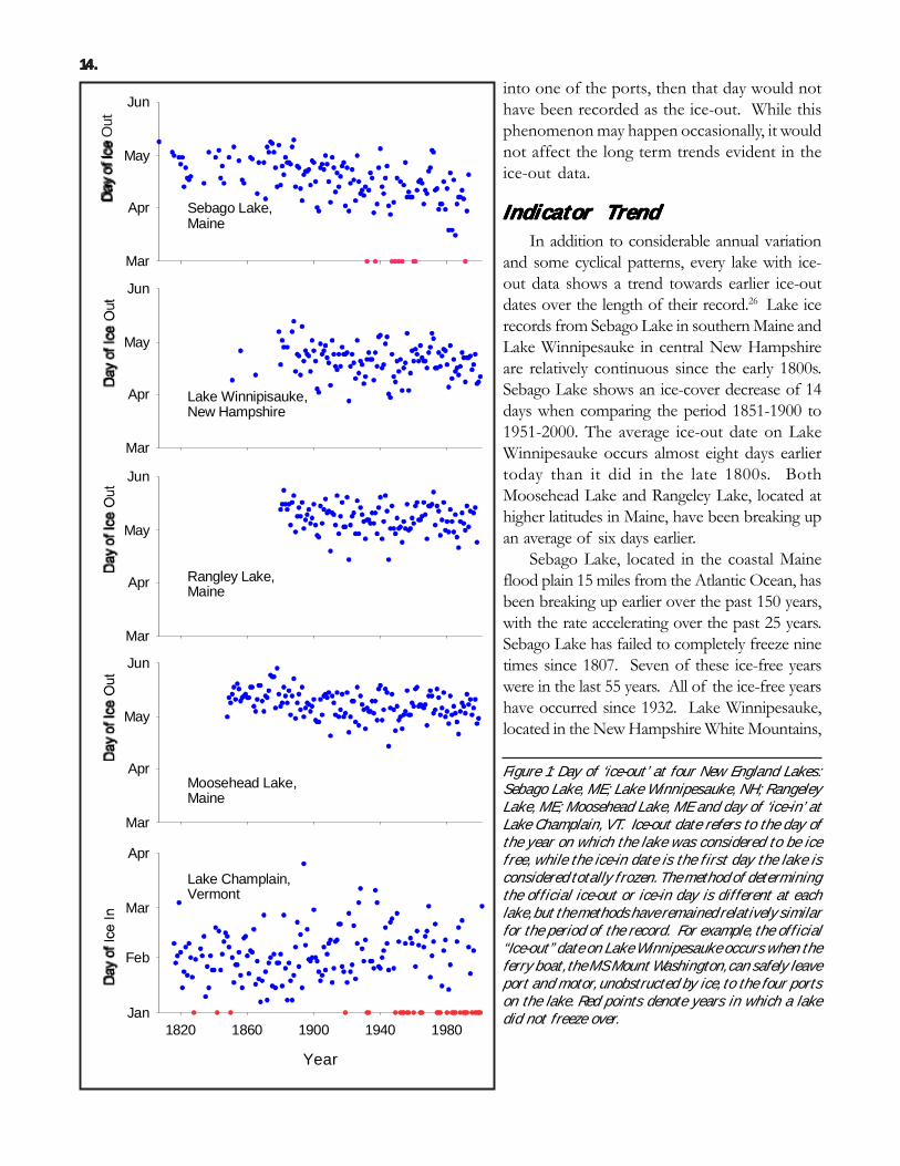
IIIIIndicndicndicndicndicaaaaatttttooooor Tr Tr Tr Tr TrrrrreeeeendndndndndIn addition to considerable annual variation

and some cyclical patterns, every lake with ice-out data shows a trend towards earlier ice-outdates over the length of their record.26 Lake icerecords from Sebago Lake in southern Maine andLake Winnipesauke in central New Hampshireare relatively continuous since the early 1800s.Sebago Lake shows an ice-cover decrease of 14days when comparing the period 1851-1900 to1951-2000. The average ice-out date on LakeWinnipesauke occurs almost eight days earliertoday than it did in the late 1800s. BothMoosehead Lake and Rangeley Lake, located athigher latitudes in Maine, have been breaking upan average of six days earlier.

Sebago Lake, located in the coastal Maineflood plain 15 miles from the Atlantic Ocean, hasbeen breaking up earlier over the past 150 years,with the rate accelerating over the past 25 years.Sebago Lake has failed to completely freeze ninetimes since 1807. Seven of these ice-free yearswere in the last 55 years. All of the ice-free yearshave occurred since 1932. Lake Winnipesauke,located in the New Hampshire White Mountains,

Figure 1: Day of ‘ice-out’ at four New England Lakes:Sebago Lake, ME; Lake Winnipesauke, NH; RangeleyLake, ME; Moosehead Lake, ME and day of ‘ice-in’ atLake Champlain, VT. Ice-out date refers to the day ofthe year on which the lake was considered to be icefree, while the ice-in date is the first day the lake isconsidered totally frozen. The method of determiningthe official ice-out or ice-in day is different at eachlake, but the methods have remained relatively similarfor the period of the record. For example, the official“Ice-out” date on Lake Winnipesauke occurs when theferry boat, the MS Mount Washington, can safely leaveport and motor, unobstructed by ice, to the four portson the lake. Red points denote years in which a lakedid not freeze over.

15.15.15.15.15.

has also broken up earlier. From 1951-2000,ice-out averaged April 20, a full week earlierthan the 1851-1900 average of April 27.

The date Lake Champlain, VT, wasfirst frozen over (‘ice-in’) has alsochanged over the past 150 years.27 Todayit freezes over 8 days later than it did inthe second half of the 1800s. But themost remarkable part of the record is theoccurrence of years in which the lake didnot freeze over all winter. Over the 186year record, the lake has not frozen overin 31 winters, 75% of which were since1900, and almost half of them occurredsince 1970 (years the lake did not freeze

are denoted in the figure with red points).In general, lakes farther from the ocean and at higher elevations show smaller decreases in the length of

ice cover. Lakes at higher latitudes show smaller but equally significant warming trends over the past 150years. Lakes with larger climate variability, those prone to inclement weather and large amounts of precipitationshow ice-out dates more statistically dependent on local events. Overall, ice-out dates were 9 days and 16days earlier between 1850 and 2000 in the northern/mountainous and southern regions of New Englandrespectively.28

Ice-out and ice-in dates recorded in the Northeast are consistent with the warming trend evident in theannual and winter temperature records over the past 100 years.

PrecipitationPrecipitationPrecipitationPrecipitationPrecipitation1900 - 20001900 - 20001900 - 20001900 - 20001900 - 2000

Indicator Overview andIndicator Overview andIndicator Overview andIndicator Overview andIndicator Overview andRRRRReeeeegggggioioioioionnnnnaaaaal Il Il Il Il Immmmmpopopopoportrtrtrtrtancancancancanceeeee

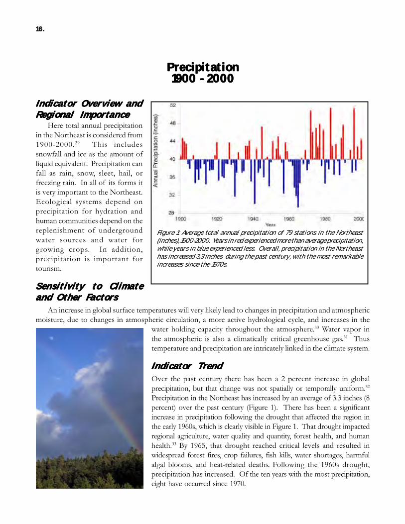
Here total annual precipitationin the Northeast is considered from1900-2000.29 This includessnowfall and ice as the amount ofliquid equivalent. Precipitation canfall as rain, snow, sleet, hail, orfreezing rain. In all of its forms itis very important to the Northeast.Ecological systems depend onprecipitation for hydration andhuman communities depend on thereplenishment of undergroundwater sources and water forgrowing crops. In addition,precipitation is important fortourism.

Sensitivity to ClimateSensitivity to ClimateSensitivity to ClimateSensitivity to ClimateSensitivity to Climateand Oand Oand Oand Oand Ottttthhhhheeeeer Fr Fr Fr Fr Factactactactactooooorrrrrsssss

An increase in global surface temperatures will very likely lead to changes in precipitation and atmosphericmoisture, due to changes in atmospheric circulation, a more active hydrological cycle, and increases in the

water holding capacity throughout the atmosphere.30 Water vapor inthe atmospheric is also a climatically critical greenhouse gas.31 Thustemperature and precipitation are intricately linked in the climate system.

IIIIIndicndicndicndicndicaaaaatttttooooor Tr Tr Tr Tr TrrrrreeeeendndndndndOver the past century there has been a 2 percent increase in globalprecipitation, but that change was not spatially or temporally uniform.32

Precipitation in the Northeast has increased by an average of 3.3 inches (8percent) over the past century (Figure 1). There has been a significantincrease in precipitation following the drought that affected the region inthe early 1960s, which is clearly visible in Figure 1. That drought impactedregional agriculture, water quality and quantity, forest health, and humanhealth.33 By 1965, that drought reached critical levels and resulted inwidespread forest fires, crop failures, fish kills, water shortages, harmfulalgal blooms, and heat-related deaths. Following the 1960s drought,precipitation has increased. Of the ten years with the most precipitation,eight have occurred since 1970.

Figure 1: Average total annual precipitation of 79 stations in the Northeast(inches), 1900-2000. Years in red experienced more than average precipitation,while years in blue experienced less. Overall, precipitation in the Northeasthas increased 3.3 inches during the past century, with the most remarkableincreases since the 1970s.

1 6 .1 6 .1 6 .1 6 .1 6 .

17 .17 .17 .17 .17 .

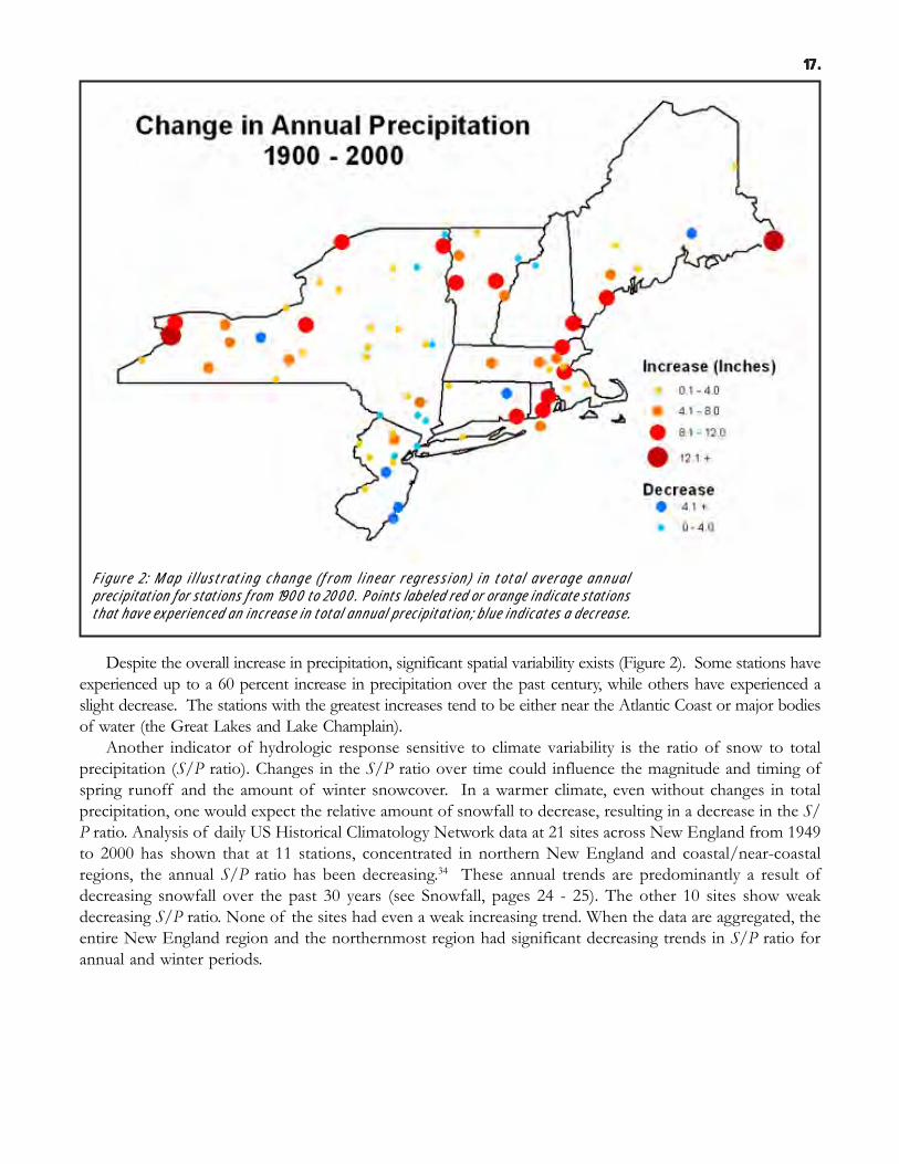
Despite the overall increase in precipitation, significant spatial variability exists (Figure 2). Some stations haveexperienced up to a 60 percent increase in precipitation over the past century, while others have experienced aslight decrease. The stations with the greatest increases tend to be either near the Atlantic Coast or major bodiesof water (the Great Lakes and Lake Champlain).

Another indicator of hydrologic response sensitive to climate variability is the ratio of snow to totalprecipitation (S/P ratio). Changes in the S/P ratio over time could influence the magnitude and timing ofspring runoff and the amount of winter snowcover. In a warmer climate, even without changes in totalprecipitation, one would expect the relative amount of snowfall to decrease, resulting in a decrease in the S/P ratio. Analysis of daily US Historical Climatology Network data at 21 sites across New England from 1949to 2000 has shown that at 11 stations, concentrated in northern New England and coastal/near-coastalregions, the annual S/P ratio has been decreasing.34 These annual trends are predominantly a result ofdecreasing snowfall over the past 30 years (see Snowfall, pages 24 - 25). The other 10 sites show weakdecreasing S/P ratio. None of the sites had even a weak increasing trend. When the data are aggregated, theentire New England region and the northernmost region had significant decreasing trends in S/P ratio forannual and winter periods.

Figure 2: Map illustrating change (from linear regression) in total average annualprecipitation for stations from 1900 to 2000. Points labeled red or orange indicate stationsthat have experienced an increase in total annual precipitation; blue indicates a decrease.

IIIIInnnnntttttense Pense Pense Pense Pense Prrrrrecieciecieciecipitpitpitpitpitatatatatatioioioioion En En En En Evvvvvenenenenentststststs1888 - 20001888 - 20001888 - 20001888 - 20001888 - 2000

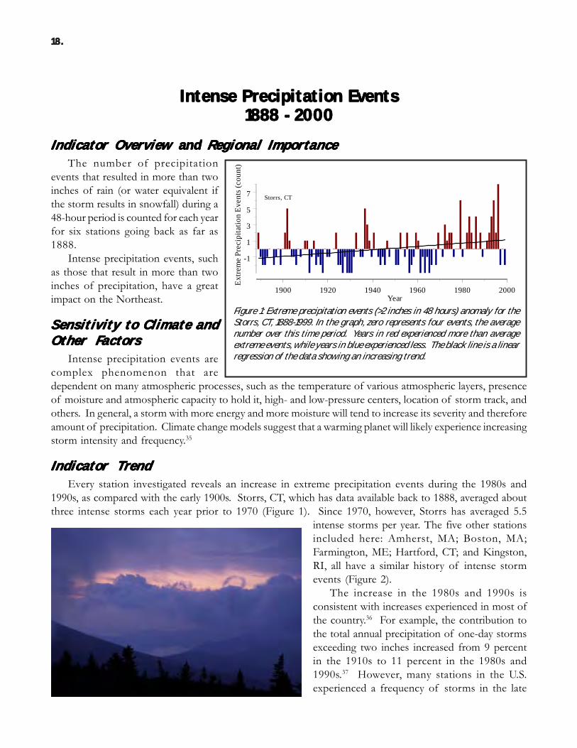
IIIIIndicndicndicndicndicaaaaatttttooooor Or Or Or Or Ovvvvveeeeervrvrvrvrvieieieieiew w w w w and and and and and RRRRReeeeegggggioioioioionnnnnaaaaal Il Il Il Il ImmmmmpopopopoportrtrtrtrtancancancancanceeeeeThe number of precipitation

events that resulted in more than twoinches of rain (or water equivalent ifthe storm results in snowfall) during a48-hour period is counted for each yearfor six stations going back as far as1888.

Intense precipitation events, suchas those that result in more than twoinches of precipitation, have a greatimpact on the Northeast.

Sensitivity to Climate andSensitivity to Climate andSensitivity to Climate andSensitivity to Climate andSensitivity to Climate andOOOOOttttthhhhheeeeer Fr Fr Fr Fr Factactactactactooooorrrrrsssss

Intense precipitation events arecomplex phenomenon that aredependent on many atmospheric processes, such as the temperature of various atmospheric layers, presenceof moisture and atmospheric capacity to hold it, high- and low-pressure centers, location of storm track, andothers. In general, a storm with more energy and more moisture will tend to increase its severity and thereforeamount of precipitation. Climate change models suggest that a warming planet will likely experience increasingstorm intensity and frequency.35

IIIIIndicndicndicndicndicaaaaatttttooooor Tr Tr Tr Tr TrrrrreeeeendndndndndEvery station investigated reveals an increase in extreme precipitation events during the 1980s and

1990s, as compared with the early 1900s. Storrs, CT, which has data available back to 1888, averaged aboutthree intense storms each year prior to 1970 (Figure 1). Since 1970, however, Storrs has averaged 5.5

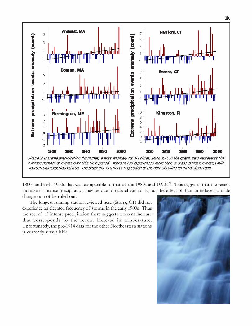
intense storms per year. The five other stationsincluded here: Amherst, MA; Boston, MA;Farmington, ME; Hartford, CT; and Kingston,RI, all have a similar history of intense stormevents (Figure 2).

The increase in the 1980s and 1990s isconsistent with increases experienced in most ofthe country.36 For example, the contribution tothe total annual precipitation of one-day stormsexceeding two inches increased from 9 percentin the 1910s to 11 percent in the 1980s and1990s.37 However, many stations in the U.S.experienced a frequency of storms in the late

1 8 .1 8 .1 8 .1 8 .1 8 .

-1

1

3

5

7

Extre

me

Prec

ipita

tion

Even

ts (c

ount

)

Storrs, CT

1900 1920 1940 1960 1980 2000Year

Figure 1: Extreme precipitation events (>2 inches in 48 hours) anomaly for theStorrs, CT, 1888-1999. In the graph, zero represents four events, the averagenumber over this time period. Years in red experienced more than averageextreme events, while years in blue experienced less. The black line is a linearregression of the data showing an increasing trend.

1 9 .1 9 .1 9 .1 9 .1 9 .

Figure 2: Extreme precipitation (>2 inches) events anomaly for six cities, 1914-2000. In the graph, zero represents theaverage number of events over this time period. Years in red experienced more than average extreme events, whileyears in blue experienced less. The black line is a linear regression of the data showing an increasing trend.

19201920192019201920 1940 1940 1940 1940 1940 1960 1960 1960 1960 1960 1980 20001980 20001980 20001980 20001980 2000 1920 1920 1920 1920 1920 1940 1940 1940 1940 1940 1960 1960 1960 1960 1960 1980 20001980 20001980 20001980 20001980 2000

Ex

tre

me

pre

cip

ita

tio

n e

ven

ts a

no

ma

ly (

cou

nt)

Ex

tre

me

pre

cip

ita

tio

n e

ven

ts a

no

ma

ly (

cou

nt)

Ex

tre

me

pre

cip

ita

tio

n e

ven

ts a

no

ma

ly (

cou

nt)

Ex

tre

me

pre

cip

ita

tio

n e

ven

ts a

no

ma

ly (

cou

nt)

Ex

tre

me

pre

cip

ita

tio

n e

ven

ts a

no

ma

ly (

cou

nt)

-1

1

3

5

7 Hartford, CT

-1

1

3

5

7Storrs, CT

-2

0

2

4

6

8

10Kingston, RI

HHHHHartfartfartfartfartfororororord,d,d,d,d, CT CT CT CT CT

Storrs, CTStorrs, CTStorrs, CTStorrs, CTStorrs, CT

KKKKKininininingstgstgstgstgstooooon,n,n,n,n, R R R R RIIIII

Ex

tre

me

pre

cip

ita

tio

n e

ven

ts a

no

ma

ly (

cou

nt)

Ex

tre

me

pre

cip

ita

tio

n e

ven

ts a

no

ma

ly (

cou

nt)

Ex

tre

me

pre

cip

ita

tio

n e

ven

ts a

no

ma

ly (

cou

nt)

Ex

tre

me

pre

cip

ita

tio

n e

ven

ts a

no

ma

ly (

cou

nt)

Ex

tre

me

pre

cip

ita

tio

n e

ven

ts a

no

ma

ly (

cou

nt)

-1

1

3

5Amherst, MA

-1

1

3

5Boston, MA

-2

-1

0

1

2

3 Farmington, ME

Amherst, MA Amherst, MA Amherst, MA Amherst, MA Amherst, MA

Boston, MABoston, MABoston, MABoston, MABoston, MA

FFFFFarararararmmmmmininininingtgtgtgtgtooooon,n,n,n,n, ME ME ME ME ME

1800s and early 1900s that was comparable to that of the 1980s and 1990s.38 This suggests that the recentincrease in intense precipitation may be due to natural variability, but the effect of human induced climatechange cannot be ruled out.

The longest running station reviewed here (Storrs, CT) did notexperience an elevated frequency of storms in the early 1900s. Thusthe record of intense precipitation there suggests a recent increasethat corresponds to the recent increase in temperature.Unfortunately, the pre-1914 data for the other Northeastern stationsis currently unavailable.

Sea Level RiseSea Level RiseSea Level RiseSea Level RiseSea Level Rise1856-20001856-20001856-20001856-20001856-2000

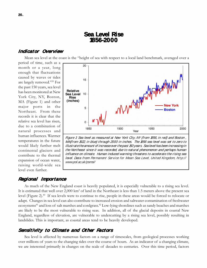
Indicator OverviewIndicator OverviewIndicator OverviewIndicator OverviewIndicator OverviewMean sea level at the coast is the “height of sea with respect to a local land benchmark, averaged over a

period of time, such as amonth or a year, longenough that fluctuationscaused by waves or tidesare largely removed.”39 Forthe past 150 years, sea levelhas been monitored at NewYork City, NY, Boston,MA (Figure 1) and othermajor ports in theNortheast. From theserecords it is clear that therelative sea level has risen,due to a combination ofnatural processes andhuman influences. Warmertemperatures in the futurewould likely further meltcontinental glaciers andcontribute to the thermalexpansion of ocean water,raising world-wide sealevel even further.

RRRRReeeeegggggioioioioionnnnnaaaaal Il Il Il Il Immmmmpopopopoportrtrtrtrtancancancancanceeeee

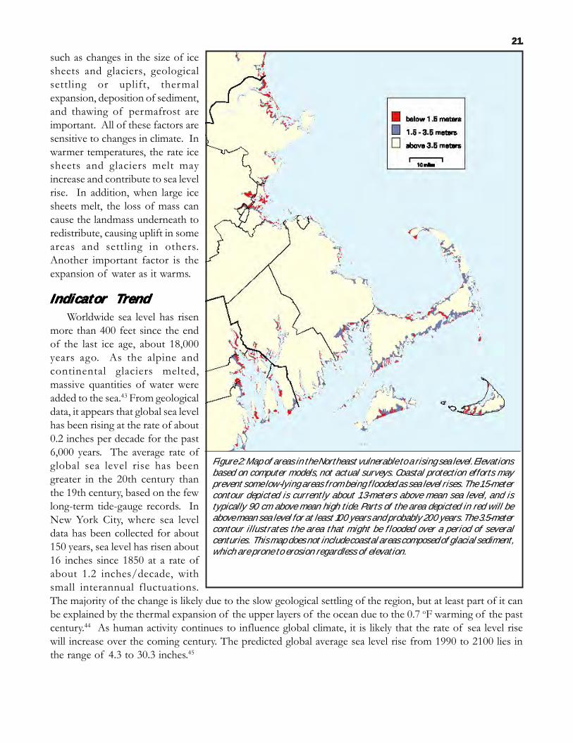
As much of the New England coast is heavily populated, it is especially vulnerable to a rising sea level.It is estimated that well over 2,000 km2 of land in the Northeast is less than 1.5 meters above the present sealevel (Figure 2).40 If sea levels were to continue to rise, people in these areas would be forced to relocate oradapt. Changes in sea level can also contribute to increased erosion and saltwater contamination of freshwaterecosystems41 and loss of salt marshes and cordgrass.42 Low-lying shorelines such as sandy beaches and marshesare likely to be the most vulnerable to rising seas. In addition, all of the glacial deposits in coastal NewEngland, regardless of elevation, are vulnerable to undercutting by a rising sea level, possibly resulting inlandslides. This is important, as coastal areas tend to be heavily developed.

SSSSSeeeeensnsnsnsnsiiiiitttttiiiiivvvvviiiiittttty ty ty ty ty to Co Co Co Co Climlimlimlimlimaaaaattttte and Oe and Oe and Oe and Oe and Ottttthhhhheeeeer Fr Fr Fr Fr FactactactactactooooorrrrrsssssSea level is affected by numerous factors on a range of timescales, from geological processes working

over millions of years to the changing tides over the course of hours. As an indicator of a changing climate,we are interested primarily in changes on the scale of decades to centuries. Over this time period, factors

20.20.20.20.20.

Figure 1: Sea level as measured at New York City, NY (from 1856, in red) and Boston ,MA(from 1922, in blue) through 2000 in inches. The 1856 sea level was set to zero toillustrate the amount of increase over the past 150 years. Sea level has been increasing inthe Northeast since it was recorded, due to natural phenomenon and perhaps humaninfluence on climate. Human induced warming threatens to accelerate the rising sealevel. Data from Permanent Service for Mean Sea Level, United Kingdom, http://www.pol.ac.uk/psmsl/

such as changes in the size of icesheets and glaciers, geologicalsettling or uplift, thermalexpansion, deposition of sediment,and thawing of permafrost areimportant. All of these factors aresensitive to changes in climate. Inwarmer temperatures, the rate icesheets and glaciers melt mayincrease and contribute to sea levelrise. In addition, when large icesheets melt, the loss of mass cancause the landmass underneath toredistribute, causing uplift in someareas and settling in others.Another important factor is theexpansion of water as it warms.

IIIIIndicndicndicndicndicaaaaatttttooooor Tr Tr Tr Tr TrrrrreeeeendndndndndWorldwide sea level has risen

more than 400 feet since the endof the last ice age, about 18,000years ago. As the alpine andcontinental glaciers melted,massive quantities of water wereadded to the sea.43 From geologicaldata, it appears that global sea levelhas been rising at the rate of about0.2 inches per decade for the past6,000 years. The average rate ofglobal sea level rise has beengreater in the 20th century thanthe 19th century, based on the fewlong-term tide-gauge records. InNew York City, where sea leveldata has been collected for about150 years, sea level has risen about16 inches since 1850 at a rate ofabout 1.2 inches/decade, withsmall interannual fluctuations.The majority of the change is likely due to the slow geological settling of the region, but at least part of it canbe explained by the thermal expansion of the upper layers of the ocean due to the 0.7 oF warming of the pastcentury.44 As human activity continues to influence global climate, it is likely that the rate of sea level risewill increase over the coming century. The predicted global average sea level rise from 1990 to 2100 lies inthe range of 4.3 to 30.3 inches.45

21 .21 .21 .21 .21 .

Figure 2: Map of areas in the Northeast vulnerable to a rising sea level. Elevationsbased on computer models, not actual surveys. Coastal protection efforts mayprevent some low-lying areas from being flooded as sea level rises. The 1.5-metercontour depicted is currently about 1.3-meters above mean sea level, and istypically 90 cm above mean high tide. Parts of the area depicted in red will beabove mean sea level for at least 100 years and probably 200 years. The 3.5-metercontour illustrates the area that might be flooded over a period of severalcenturies. This map does not include coastal areas composed of glacial sediment,which are prone to erosion regardless of elevation.

SSSSSea Sea Sea Sea Sea Surfurfurfurfurface Tace Tace Tace Tace Teeeeemmmmmpepepepeperrrrraturaturaturaturatureeeee1855 - 20011855 - 20011855 - 20011855 - 20011855 - 2001

Indicator OverviewIndicator OverviewIndicator OverviewIndicator OverviewIndicator OverviewSurface water temperature data

from buoys, ships and other platformsfrom the late 18th century have beenassembled, quality controlled, and madewidely available to the internationalresearch community. This indicator isa review of the historical sea surfacetemperatures (SST) from 1860-2001 forthe Gulf of Maine and the South Shoreof New England.46

RRRRReeeeegggggioioioioionnnnnaaaaal Il Il Il Il ImmmmmpopopopoportrtrtrtrtancancancancanceeeeeSea surface temperature is an

important moderator of regionalclimate. Areas near the coast generallyexperience warmer winters and coolersummers due to the vast heat storagecapacity of the ocean. SST also playsa key role in storm tracking andintensity. Here SST is presented for twomarine regions; the first is the Gulf ofMaine, off the coast of Maine and New Hampshire. The second region is the South Shore, which extendsfrom Cape Cod, Massachusetts to Long Island, New York.

22.22.22.22.22.

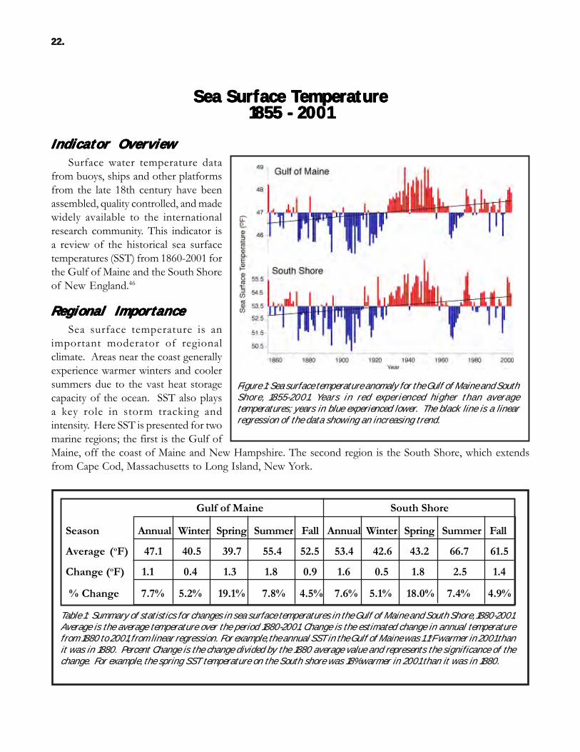
Table 1: Summary of statistics for changes in sea surface temperatures in the Gulf of Maine and South Shore, 1880-2001.Average is the average temperature over the period 1880-2001. Change is the estimated change in annual temperaturefrom 1880 to 2001, from linear regression. For example, the annual SST in the Gulf of Maine was 1.1oF warmer in 2001 thanit was in 1880. Percent Change is the change divided by the 1880 average value and represents the significance of thechange. For example, the spring SST temperature on the South shore was 18% warmer in 2001 than it was in 1880.

Gulf of Maine South Shore

Season Annual Winter Spring Summer Fall Annual Winter Spring Summer Fall

Average (oF) 47.1 40.5 39.7 55.4 52.5 53.4 42.6 43.2 66.7 61.5

Change (oF) 1.1 0.4 1.3 1.8 0.9 1.6 0.5 1.8 2.5 1.4

% Change 7.7% 5.2% 19.1% 7.8% 4.5% 7.6% 5.1% 18.0% 7.4% 4.9%

Figure 1: Sea surface temperature anomaly for the Gulf of Maine and SouthShore, 1855-2001. Years in red experienced higher than averagetemperatures; years in blue experienced lower. The black line is a linearregression of the data showing an increasing trend.

The world’s oceans are continually circulating, moving heat from the tropics to the polar regions at aboutthe same rate as the atmosphere. The oceans are huge reservoirs of heat and thus have a strong influence onglobal and regional temperature. Because of its size, the ocean changes temperature very slowly and can actas a heat sink or source, depending on the temperature of the air above it. While air temperatures can varydramatically over the course of hours, ocean water takes months to warm up or cool down significantly. Inthis way, any change in SST represents changes in temperature on a seasonal, annual, or multi-annual timeframe.

IIIIIndicndicndicndicndicaaaaatttttooooor Tr Tr Tr Tr TrrrrreeeeendndndndndBoth marine regions have experienced significant variability since the 1880s. From 1880 through the

early 1920s, the Gulf of Maine and the South Shore experienced below average temperatures. From the late1920s to the early 1950s, SST was warmer than average. Since that time, SST has mostly remained aboveaverage in the Gulf of Maine and the South Shore.

Overall the SST in these regions has warmed significantly, with an increase of 1.1 oF (8 percent) in theGulf of Maine and 1.6 oF (8 percent) on the South Shore. Most of this warming has taken place in the springand summer months, where there has been an increase of about 1.3 to 1.8oF in both locations (Table 1). These regional trends are generally consistent with global records of SST, which reveal a rapid warmingfrom 1905 to 1940 followed by a slight increase from 1940 to 2001.47

SSSSSeeeeensnsnsnsnsiiiiitttttiiiiivvvvviiiiittttty ty ty ty ty to Co Co Co Co Climlimlimlimlimaaaaattttte and Oe and Oe and Oe and Oe and Ottttthhhhheeeeer Fr Fr Fr Fr Factactactactactooooorrrrrsssss23.23.23.23.23.

SSSSSnononononowfwfwfwfwfaaaaallllllllll1880 - 20011880 - 20011880 - 20011880 - 20011880 - 2001

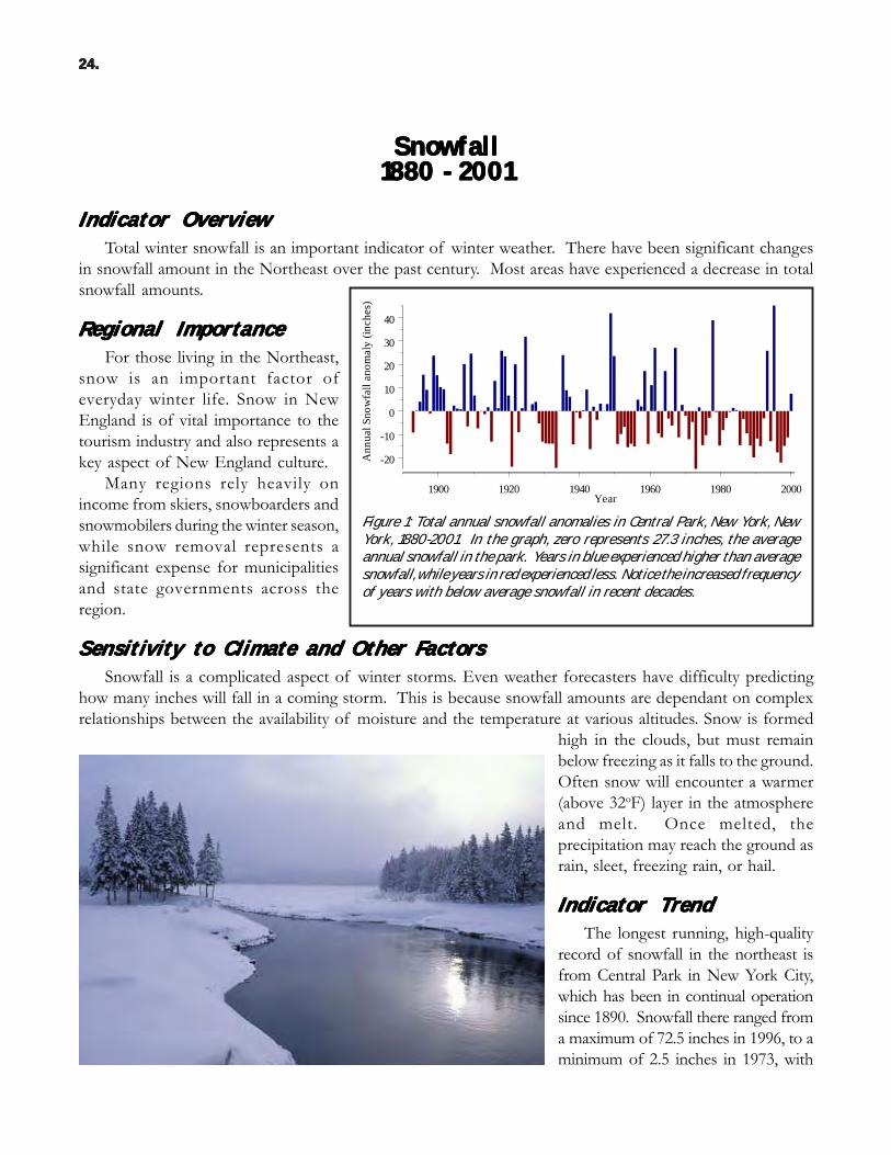
Indicator OverviewIndicator OverviewIndicator OverviewIndicator OverviewIndicator OverviewTotal winter snowfall is an important indicator of winter weather. There have been significant changes

in snowfall amount in the Northeast over the past century. Most areas have experienced a decrease in totalsnowfall amounts.

RRRRReeeeegggggioioioioionnnnnaaaaal Il Il Il Il ImmmmmpopopopoportrtrtrtrtancancancancanceeeeeFor those living in the Northeast,

snow is an important factor ofeveryday winter life. Snow in NewEngland is of vital importance to thetourism industry and also represents akey aspect of New England culture.

Many regions rely heavily onincome from skiers, snowboarders andsnowmobilers during the winter season,while snow removal represents asignificant expense for municipalitiesand state governments across theregion.

SSSSSeeeeensnsnsnsnsiiiiitttttiiiiivvvvviiiiittttty ty ty ty ty to Co Co Co Co Climlimlimlimlimaaaaattttte and Oe and Oe and Oe and Oe and Ottttthhhhheeeeer Fr Fr Fr Fr FactactactactactooooorrrrrsssssSnowfall is a complicated aspect of winter storms. Even weather forecasters have difficulty predicting

how many inches will fall in a coming storm. This is because snowfall amounts are dependant on complexrelationships between the availability of moisture and the temperature at various altitudes. Snow is formed

high in the clouds, but must remainbelow freezing as it falls to the ground.Often snow will encounter a warmer(above 32oF) layer in the atmosphereand melt. Once melted, theprecipitation may reach the ground asrain, sleet, freezing rain, or hail.

IIIIIndicndicndicndicndicaaaaatttttooooor Tr Tr Tr Tr TrrrrreeeeendndndndndThe longest running, high-quality

record of snowfall in the northeast isfrom Central Park in New York City,which has been in continual operationsince 1890. Snowfall there ranged froma maximum of 72.5 inches in 1996, to aminimum of 2.5 inches in 1973, with

24.24.24.24.24.

Year

-20

-10

0

10

20

30

40

Ann

ual S

now

fall

anom

aly

(inch

es)

1900 1920 1940 1960 1980 2000

Figure 1: Total annual snowfall anomalies in Central Park, New York, NewYork, 1880-2001. In the graph, zero represents 27.3 inches, the averageannual snowfall in the park. Years in blue experienced higher than averagesnowfall, while years in red experienced less. Notice the increased frequencyof years with below average snowfall in recent decades.

25.25.25.25.25.

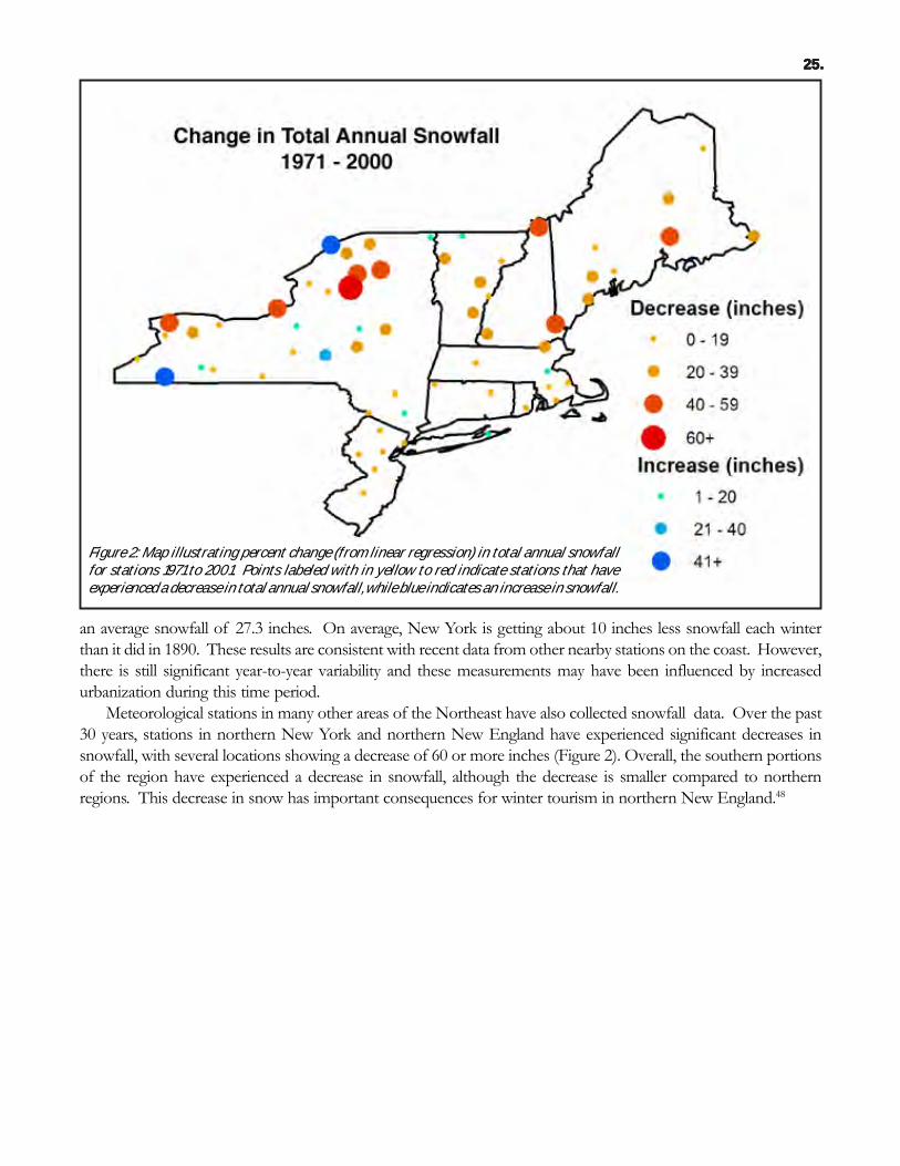
an average snowfall of 27.3 inches. On average, New York is getting about 10 inches less snowfall each winterthan it did in 1890. These results are consistent with recent data from other nearby stations on the coast. However,there is still significant year-to-year variability and these measurements may have been influenced by increasedurbanization during this time period.

Meteorological stations in many other areas of the Northeast have also collected snowfall data. Over the past30 years, stations in northern New York and northern New England have experienced significant decreases insnowfall, with several locations showing a decrease of 60 or more inches (Figure 2). Overall, the southern portionsof the region have experienced a decrease in snowfall, although the decrease is smaller compared to northernregions. This decrease in snow has important consequences for winter tourism in northern New England.48

Figure 2: Map illustrating percent change (from linear regression) in total annual snowfallfor stations 1971 to 2001. Points labeled with in yellow to red indicate stations that haveexperienced a decrease in total annual snowfall, while blue indicates an increase in snowfall.

DDDDDaaaaayyyyys ws ws ws ws wititititith Sh Sh Sh Sh Snononononow ow ow ow ow on Grn Grn Grn Grn Groooooundundundundund1970 - 20011970 - 20011970 - 20011970 - 20011970 - 2001

Indicator OverviewIndicator OverviewIndicator OverviewIndicator OverviewIndicator OverviewLike total snowfall, total days with snow on the ground are an important indicator of winter weather.

Unfortunately, few meteorological stations have been recording the presence of snow on the ground for verylong. As a result, this indicator is onlyavailable for many stations back to1970.

RRRRReeeeegggggioioioioionnnnnaaaaal Il Il Il Il ImmmmmpopopopoportrtrtrtrtancancancancanceeeeeThis indicator is perhaps more

relevant to outdoor recreation thantotal snowfall, because it is a measureof the length of the winter recreationseason. While the total amount ofsnow is important, the length of timeit stays is also a significant factor. Manyforms of winter recreation, such asskiing and snowmobiling, rely on snowcover. In addition, snow affectsecological systems. Snow depth andpersistence of snow cover areimportant factors in the reproductionand growth of plants.49

SSSSSeeeeensnsnsnsnsiiiiitttttiiiiivvvvviiiiittttty ty ty ty ty to Co Co Co Co Climlimlimlimlimaaaaattttte and Oe and Oe and Oe and Oe and Ottttthhhhheeeeer Fr Fr Fr Fr FactactactactactooooorrrrrsssssThe total number of days with snow on the ground for a given year is sensitive to both snowfall

amounts and temperature fluctuations. For example, a single storm may drop two feet of snow in a region,but it could melt in three days of warmweather. Thus snow-on-ground is a usefulindicator of overall winter severity.

IIIIIndicndicndicndicndicaaaaatttttooooor Tr Tr Tr Tr TrrrrreeeeendndndndndSatellite records indicate that snow

cover extent (SCE) in the NorthernHemisphere has decreased by about 10%since 1966 and is strongly related toincreases in temperature.50 Snowfall in theNortheast is extremely variable, withsome stations receiving only a few inchesof snow and others receiving more than100 inches every year. Thus the number of

2 6 .2 6 .2 6 .2 6 .2 6 .

Year

-30

-10

10

30

Day

s with

snow

on

grou

nd (a

nom

olie

s)

1970 1980 1990 2000

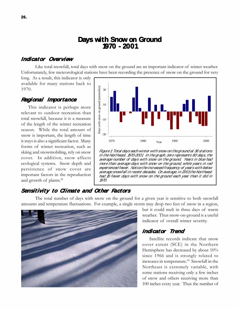
Figure 1: Total days each winter with snow on the ground at 36 stations in the Northeast, 1970-2001. In the graph, zero represents 80 days, the average number of days with snow on the ground. Years in blue had more than average days with snow on the ground, while years in red experienced fewer. Notice the increased frequency of years with below average snowfall in recent decades. On average, in 2001 the Northeast had 16 fewer days with snow on the ground each year than it did in 1970.

27.27 .27 .27 .27 .

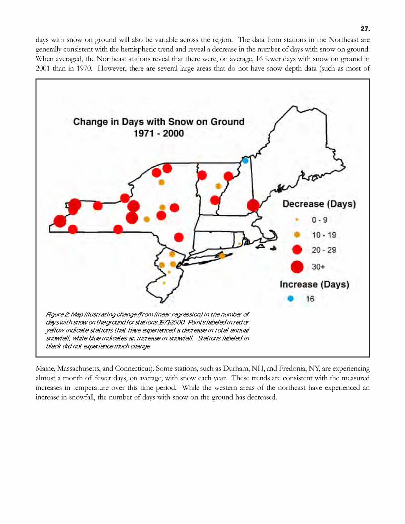
days with snow on ground will also be variable across the region. The data from stations in the Northeast aregenerally consistent with the hemispheric trend and reveal a decrease in the number of days with snow on ground.When averaged, the Northeast stations reveal that there were, on average, 16 fewer days with snow on ground in2001 than in 1970. However, there are several large areas that do not have snow depth data (such as most of

Maine, Massachusetts, and Connecticut). Some stations, such as Durham, NH, and Fredonia, NY, are experiencingalmost a month of fewer days, on average, with snow each year. These trends are consistent with the measuredincreases in temperature over this time period. While the western areas of the northeast have experienced anincrease in snowfall, the number of days with snow on the ground has decreased.

Figure 2: Map illustrating change (from linear regression) in the number ofdays with snow on the ground for stations 1971-2000. Points labeled in red oryellow indicate stations that have experienced a decrease in total annualsnowfall, while blue indicates an increase in snowfall. Stations labeled inblack did not experience much change.

SSSSSUMMUMMUMMUMMUMMAAAAARRRRRYYYYY

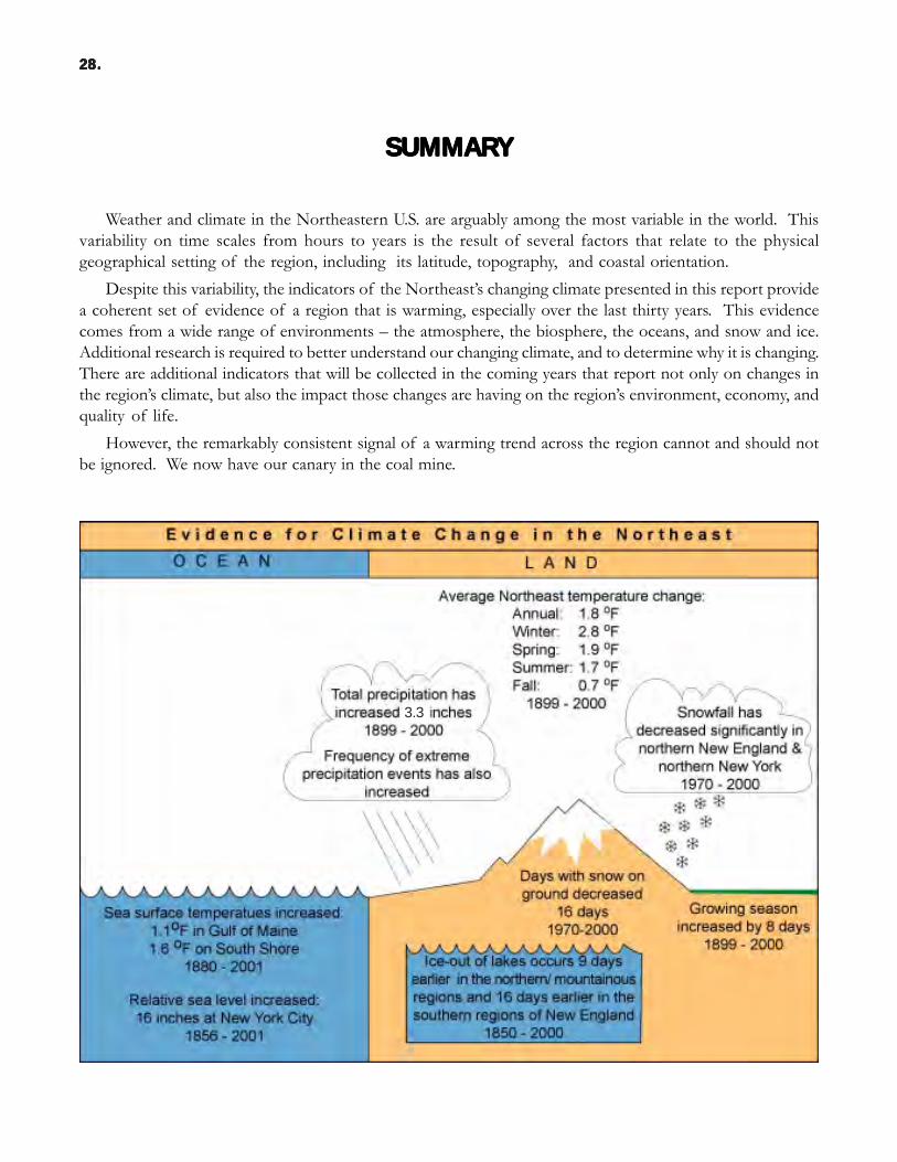
Weather and climate in the Northeastern U.S. are arguably among the most variable in the world. Thisvariability on time scales from hours to years is the result of several factors that relate to the physicalgeographical setting of the region, including its latitude, topography, and coastal orientation.

Despite this variability, the indicators of the Northeast’s changing climate presented in this report providea coherent set of evidence of a region that is warming, especially over the last thirty years. This evidencecomes from a wide range of environments – the atmosphere, the biosphere, the oceans, and snow and ice.Additional research is required to better understand our changing climate, and to determine why it is changing.There are additional indicators that will be collected in the coming years that report not only on changes inthe region’s climate, but also the impact those changes are having on the region’s environment, economy, andquality of life.

However, the remarkably consistent signal of a warming trend across the region cannot and should notbe ignored. We now have our canary in the coal mine.

2 8 .2 8 .2 8 .2 8 .2 8 .

3.3

2 9 .2 9 .2 9 .2 9 .2 9 .

RRRRReeeeefffffeeeeerrrrrencesencesencesencesences

30.30.30.30.30.

1 The data used in this analysis is from the National Climatic Data Center (ftp://ftp.ncdc.noaa.gov/pub/data/ushcn/). The series for the New England region comprises areally weighted values. The station data were firstaveraged by climate division. Then the climate division data were averaged, giving proportional weight to the largerdivisions. The mean of the series is 44.6 oF. Keim, B.D., A. Wilson, C. Wake, and T.G. Huntington. 2003. Are therespurious temperature trends in the United States Climate Division Database? Geophys. Res. Lett. 30(27), 1404,doi:10.1029/2002GL016295 30:1404, doi:10.1029/2002GL016295.Trombulak, S.C., and R. Wolfson. 2004.Twentieth-century climate change in New England and New York, USA. J. Geophys. Res. 31:L19202, doi:10.1029/2004GL020574.2 “Speech on the Weather” was given at the New England Society’s seventy-first annual dinner, in New York City onDecember 22, 1876. From The Family Mark Twain, New York: Harper & Row, 1975.3 Climate Change 2001: The Scientific Basis. Intergovernmental Panel on Climate Change. Cambridge University Press,UK. 2001. http://www.ipcc.ch4 Frich, P., L.V. Alexander, P. Della-Marta, B. Gleason, M. Haylock, A.M.G. Klein-Tank, and T.C. Peterson. 2002.Observed coherent changes in climatic extremes during the second half of the twentieth century. Clim. Res. 19:193-212. Kunkel, K.E., Easterling, D.R., Hubbard, K., Redmond, K., 2004. Temporal variations in frost-free season in theUnited States: 1895–2000. Geophys. Res. Lett. 31, L03201, doi: 10.1029/2003 GL0186. Cooter, E.J., and S. LeDuc.1995. Recent frost date trends in the Northeastern U.S. Intl. J. Climatol. 15:65-75.5 US National Assessment of the Potential Consequences of Climate Variability and Change Educational ResourcesRegional Paper: The Northeast. US Climate Change Science Program. http://www.usgcrp.gov/usgcrp/nacc/education/northeast/ (2003). Parmesan, C., and G. Yohe. 2003. A globally coherent fingerprint of climate changeimpacts across natural systems. Nature 421:37-42. Walther, G.-P., E. Post, P. Convey, A. Menzel, C. Parmesan, T.J.C.Beebee, J.-M. Fromentin, O. Hoegh-Guldberg, and F. Bairlein. 2002. Ecological responses to recent climate change.Nature 416:389-395.6 Ricklefs, R. The Economy of Nature, 4th ed. W.H. Freeman and Company. New York. (1997)7 Baron, W. and D. Smith. Growing Season Parameter Reconstructions for New England Using Killing Frost Records, 1697 - 1947.Maine Agricultural And Forest Experimental Station Bulletin 846, University of Maine, Orono. (1996).8 The stations included in this average are Atlantic City, NJ; Blue Hill, MA; Burlington, VT; Eastport, ME; New Brunswick,NJ; Central Park, NY; and Storrs, CT. All data from the United States Historical Climate Network daily dataset, whichis available at: http://www.ncdc.noaa.gov/oa/climate/research/ushcn/daily.html9 Wolfe, D.W., M.D. Schwartz, A.N. Lakso, Y. Otsuki, R.M. Poole, N.J. Shaulis. 2005. Climate change and shifts in springphenology of three horticultural woody perennials in the northeastern United States. International Journal ofBiometeorology (in press).10 Weltsin, J.F., R.T. Belote, N.J. Sanders. 2003. Biological invaders in a greenhouse world: will elevated CO2 fuel plantinvasions? Frontiers in Ecology and Environment1(3):146-153. Thomas, C.D. et al. 2004. Extinction risk from climatechange. Nature 427: 145-148.11 Van Vliet, A.J.H., A. Overeem, R.S. Groot, A.F.G. Jacobs, and F.T.M. Spieksma. 2002. The influence oftemperature and climate change on the timing of pollen release in the Netherlands. Intl. J. Climatology 22:1757-1767.Jager, S, 2003, Global warming: trends in start, duration and intensity of the pollen seasons in Europe. Allergo J.12:314-315. Ziska, L.H., D.E. Gebhard, D.A. Frenz, S. Faulkner, B.D. Singer, and J.G. Straka. 2003. Cities asharbingers of climate change: Common ragweed, urbanization and public health. J of Allergy and Clinical Immunology111:290-295.

31 .31 .31 .31 .31 .

12 Ziska L, F. Caulfield. 2000. The potential influence of rising CO2 on public health: pollen production of thecommon ragweed as a test case. World Research Reviews 12: 449-457.13 Aono, Y. 1998. Climate change in March temperature deduced from phenologocal record for flowering ofcherry tree in Tokyo since the late 18th century. Bull. Osaka Prefecture University, Ser.B 50:11-19. Aono, Y., and Y.Omo. 1994. Estimation of temperature at Kyoto since the 11th century using flowering data of cherry trees in olddocuments. J. Agric. Meteorology 49:263-272.14 Walther, G.-R. et al. 2002. Ecological responses to recent climate change. Nature 416:389-395.15 Bradley, N.L., A.C. Leopold, J. Ross, W. Huffaker. 1999. Phenological changes reflect climate change in Wisconsin.Proceedings National Academy of Sciences USA 96:9701-9704.16 Abu-Asab, M.S. et al. 2001. Earlier plant flowering in spring as a response to global warming in the WashingtonD.C. area. Biodiversity and Conservation. 10:597-612.17 Hopp, R.J. 1974. Plant phenology observation networks. IN: Leith, H. (ed.) Phenology and Seasonality Modeling. Springer-Verlag, Heidelberg, pp. 25-43.18 A. Lakso, Cornell University, personal communication19 Zhou, L. et al. 2001. Variations in northern vegetation activity inferred from satellite data of vegetation indexduring 1981-99. Journal Geophysical Research 16:20069-20083. Zhou, L., R.K. Kaufmann, Y. Tian, C.J. Tucker, and R.B.Myneni. 2003. Relation between interannual variations in satellite measurements of northern forest greenness andclimate between 1982 and 1999. J. Geophys. Res. Atmos. 108(D):4004, doi:10.1029/2002JD002510.20 See: European phenology network site: www.dow.wau.nl/msa/epn; UK site: www.phenology.org.uk; and lilacphenology site in development for the U.S.: www.uwm.edu/~mds/markph.html.21 Prowse, T. D.: 1994, ‘Environmental significance of ice to streamflow in cold regions,’ Freshwater Biol. 32:241–259.22 Hodgkins, G A, R. W. Dudley, and T. G. Huntington. 2003. Changes in the timing of high river flows in NewEngland over the 20th century. Journal of Hydrology 278:244 - 252.23 Hodgkins, G A, R. W. Dudley, and T. G. Huntington. In Press, Changes in the number and timing of ice-affectedflow days on New England rivers, 1930-2000. Climatic Change.24 Huntington, T. G., G. A. Hodgkins, B. D. Keim, R.W. Dudley, 2004. Changes in the proportion of precipitationoccurring as snow in New England (1949 to 2000), Journal of Climate 17:2626-2636.25 IPCC, Climate Change 2001:The Science of Climate Change. Cambridge University Press, NY, NY. 200126 New England Regional Assessment Group, Preparing for a Changing Climate, New England Regional Overview, U.S.Global Change Research Program, 96 pp., University of New Hampshire. (2001)27 Hodgkins, Glenn A., Ivan C. James II, and Thomas G. Huntington, 2002: Historical changes in lake ice-out datesas indicators of climate change in New England, 1850-2000. Int. J. Climatol., 22 (15), 1819-1827.28 http://www.erh.noaa.gov/er/btv/climo/lakeclose.html29 Keim, Barry D., Fischer, Michelle Russo, Wilson, Adam M. 2005. Are there spurious precipitation trends in theUnited States Climate Division database? Geophys. Res. Lett., Vol. 32, No. 4, L04702 10.1029/2004GL021985.30 Held, I.M., and B.J. Soden. 2000. Water vapor feedback and global warming. Annual Review of Energy and theEnvironment 25:441-475.31 Climate Change 2001: The Scientific Basis. Intergovernmental Panel on Climate Change. Cambridge University Press,UK. 2001. Section 2.5.1. http://www.ipcc.ch32 Climate Change 2001: The Scientific Basis. Intergovernmental Panel on Climate Change. Cambridge University Press,UK. 2001. Section 2.5.2.1. http://www.ipcc.ch

33 The New England Regional Assessment: Key Issues and Relevant Case Studies. US Global Change Research Program.http://www.necci.sr.unh.edu/reports.html34 Huntington, T. G., G.A. Hodgkins, B.D. Keim, and R.W. Dudley. (2004) Changes in the proportion ofprecipitation occurring as snow in New England (1949 to 2000). Journal of Climate, 17, 2626-2636.35 Climate Change 2001: The Scientific Basis. Intergovernmental Panel on Climate Change. Cambridge University Press,UK. 2001.pp 572-576. http://www.ipcc.ch36 Groisman, P.Y., R.W. Knight, T.R. Karl, D.R. Easterling, B. Sun, and J. Lawrimore. 2004. Contemporary changesof the hydrological cycle over the contiguous United States: Trends. J. Hydrometeor. 5:64–85.37 Karl, T. R., R. W. Knight, D. R. Easterling, and R. G. Quayle, Trends in U.S. climate during the twentieth century,Consequences, 1, 3 – 12, 1995.38 Kunkel, K. E., D. R. Easterling, K. Redmond, and K. Hubbard, Temporal variations of extreme precipitationevents in the United States: 1895–2000, Geophys. Res. Lett., 30(17), 1900, doi:10.1029/2003GL018052, 2003.39 Climate Change 2001: The Scientific Basis. Intergovernmental Panel on Climate Change. Cambridge University Press,UK. 2001. http://www.ipcc.ch40 J.G.Titus and C.Richman, 2000, “Maps of Lands Vulnerable to Sea Level Rise: Modeled Elevations Along theU.S. Atlantic and Gulf Coasts.” Climate Research (in press)41 Climate Change 2001: The Scientific Basis. Intergovernmental Panel on Climate Change. Cambridge University Press,UK. 2001. http://www.ipcc.ch42 Donnelly, J.P., and M.D. Bertness. 2001. Rapid shoreward encroachment of salt marsh cordgrass in response toaccelerated sea-level rise. Proc. Natl Acad. Sci. 98:14218-14223.43 Climate Change 2001: The Scientific Basis. Intergovernmental Panel on Climate Change. Cambridge University Press,UK. 2001. http://www.ipcc.ch44 Barth, M. and J. Titus. Greenhouse Effect and Sea Level Rise: A Challenge for this Generation. Van Nostrand ReinholdCompany Inc, (1984)45 Climate Change 2001: The Scientific Basis. Intergovernmental Panel on Climate Change. Cambridge University Press,UK. 2001. http://www.ipcc.ch46 NOAA Extended Reconstructed SST data provided by the NOAA-CIRES Climate Diagnostics Center,Boulder, Colorado, USA, www.cdc.noaa.gov. For details on the dataset, see Smith, T.M., and R.W. Reynolds, 2003:Extended Reconstruction of Global Sea Surface Temperatures Based on COADS Data (1854-1997). Journal ofClimate, 16, 1495-1510.47 Smith, T.M., and R.W. Reynolds, 2003: Extended Reconstruction of Global Sea Surface Temperatures Based onCOADS Data (1854-1997). Journal of Climate, 16, 1495-1510.48 Hamilton, L.C., D.E. Rohall, C. Brown, G. Hayward, and B.D. Keim. 2003. Warming winters and NewHampshire’s lost ski areas: An Integrated Case Study. International Journal of Sociology and Social Policy 23: 52-73.49 Post, E., and N. Stenseth. Climatic variability, plant phenology, and northern ungulates. Ecology 80:1322-1339(1999)50 Climate Change 2001: The Scientific Basis. Intergovernmental Panel on Climate Change. Cambridge University Press,UK. 2001.pp 123-124. http://www.ipcc.ch

32.32.32.32.32.

100 Market Street, Suite 204, Portsmouth, NH 03801161 Cherry Street, New Canaan, CT 06840

603-422-6464 • 203-966-5429www.cleanair-coolplanet.org