using climate impacts indicators to evaluate climate model ... · using climate impacts indicators...

Using climate impacts indicators to evaluate climate modelensembles: temperature suitability of premium winegrapecultivation in the United States

Noah S. Diffenbaugh • Martin Scherer

Received: 31 October 2011 / Accepted: 20 April 2012 / Published online: 18 May 2012

� Springer-Verlag 2012

Abstract We explore the potential to improve under-

standing of the climate system by directly targeting climate

model analyses at specific indicators of climate change

impact. Using the temperature suitability of premium

winegrape cultivation as a climate impacts indicator, we

quantify the inter- and intra-ensemble spread in three cli-

mate model ensembles: a physically uniform multi-mem-

ber ensemble consisting of the RegCM3 high-resolution

climate model nested within the NCAR CCSM3 global

climate model; the multi-model NARCCAP ensemble

consisting of single realizations of multiple high-resolution

climate models nested within multiple global climate

models; and the multi-model CMIP3 ensemble consisting

of realizations of multiple global climate models. We find

that the temperature suitability for premium winegrape

cultivation is substantially reduced throughout the high-

value growing areas of California and the Columbia Valley

region (eastern Oregon and Washington) in all three

ensembles in response to changes in temperature projected

for the mid-twenty first century period. The reductions in

temperature suitability are driven primarily by projected

increases in mean growing season temperature and occur-

rence of growing season severe hot days. The intra-

ensemble spread in the simulated climate change impact

is smaller in the single-model ensemble than in the

multi-model ensembles, suggesting that the uncertainty

arising from internal climate system variability is smaller

than the uncertainty arising from climate model formula-

tion. In addition, the intra-ensemble spread is similar in the

NARCCAP nested climate model ensemble and the CMIP3

global climate model ensemble, suggesting that the

uncertainty arising from the model formulation of fine-

scale climate processes is not smaller than the uncertainty

arising from the formulation of large-scale climate pro-

cesses. Correction of climate model biases substantially

reduces both the inter- and intra-ensemble spread in

projected climate change impact, particularly for the multi-

model ensembles, suggesting that—at least for some sys-

tems—the projected impacts of climate change could be

more robust than the projected climate change. Extension

of this impacts-based analysis to a larger suite of impacts

indicators will deepen our understanding of future climate

change uncertainty by focusing on the climate phenomena

that most directly influence natural and human systems.

Keywords Climate change � Climate impacts � CMIP3 �NARCCAP � RegCM3 � Winegrape

1 Introduction

Although it is clearly established that increasing concen-

trations of atmospheric greenhouse gases increase the

radiative forcing of the climate system and the global-mean

surface temperature of the planet (IPCC 2007), there

remain a number of important uncertainties about the

response of the climate system to elevated greenhouse

forcing. These uncertainties include the magnitude of the

global-scale temperature response to a given level of

forcing (e.g., Knutti et al. 2008; Knutti and Hegerl 2008;

N. S. Diffenbaugh (&) � M. Scherer

Department of Environmental Earth System Science,

Woods Institute for the Environment, Stanford University,

473 Via Ortega, Stanford, CA 94305-4216, USA

e-mail: [email protected]

N. S. Diffenbaugh

Department of Earth and Atmospheric Sciences,

Purdue Climate Change Research Center,

Purdue University, West Lafayette, IN, USA

123

Clim Dyn (2013) 40:709–729

DOI 10.1007/s00382-012-1377-1

Zickfeld et al. 2009), the response of the large-scale cli-

mate dynamics to changes in the global-scale energy bal-

ance (e.g., Neelin et al. 2006; Yamaguchi and Noda 2006;

Annamalai et al. 2007) and the response of fine-scale cli-

mate dynamics to changes in the large-scale climate

dynamics (e.g., Deque et al. 2005; Diffenbaugh et al. 2005;

Gao et al. 2006; Rauscher et al. 2008; Seneviratne et al.

2010). By influencing the magnitude and/or spatial heter-

ogeneity of climate change, each of these uncertainties

presents challenges not only for predicting future climate

change, but also for predicting the impacts of that climate

change on natural and human systems (Giorgi et al. 2008).

Here we explore the potential to improve understanding

of the climate system by directly targeting analyses of

climate model ensembles at specific indicators of climate

change impact. Although climate impacts are a product of

both the climate system and a host of non-climatic condi-

tions (e.g., Kelly and Adger 2000; Adger et al. 2004; Smit

and Wandel 2006; Diffenbaugh et al. 2007; Ahmed et al.

2009), understanding the sensitivity of natural and human

systems to climate-related stresses requires understanding

of the climate phenomena that determine those stresses, as

well as the uncertainty in the response of those climate

phenomena to changes in radiative forcing. Therefore, by

focusing on the climate phenomena that most directly

influence natural and human systems, impacts indicators

can be used as a probe for analyzing the contribution of

different sources of uncertainty to the spread in future

climate projections.

Climate change uncertainty is often partitioned between

different sources based on the experimental dimensions of

the model ensemble, such as between ‘‘model’’, ‘‘scenario’’

and ‘‘internal variability’’ uncertainty in the case of the

Coupled Model Intercomparison Project (CMIP3) (Meehl

et al. 2007a) atmosphere–ocean general circulation model

(AOGCM) ensemble (Hawkins and Sutton 2009; Hawkins

and Sutton 2010). However, although many studies have

employed multi-model ensembles to analyze potential cli-

mate change impacts (e.g., Maurer 2007; Williams et al.

2007; Ahmed et al. 2009; Loarie et al. 2009; Ahmed et al.

2010; Gao et al. 2011; Pryor and Barthelmie 2011;

Rasmussen et al. 2011), and some have attempted to par-

tition the spread in the projected impacts between climatic

and non-climatic sources (e.g., Nicholls 2004; Parry et al.

2004; Tebaldi and Lobell 2008), partitioning the spread in

the projected impacts between different sources of climate

change uncertainty has received far less attention. Of par-

ticular concern is the contribution of fine-scale climate

processes, which can play a key role in shaping climate at

the spatial and temporal scales that most directly determine

climate impacts, including the frequency and magnitude of

extreme events (e.g., Christensen and Christensen 2003;

Duffy et al. 2003; Diffenbaugh et al. 2005; White et al.

2006; Rauscher et al. 2008; Diffenbaugh and Ashfaq 2010).

Although insight has been gained into the contribution of

fine-scale processes to the spread in nested climate model

ensembles, these systematic multi-model analyses have

been focused on bulk climate metrics that are not imme-

diately translatable into the impacts domain (e.g., Deque

et al. 2005; Marengo et al. 2009).

Impacts-targeted climate model analysis can provide

particular insight into the influence of climate model biases

on the ensemble spread. Assessment of climate model

errors is routine (e.g., Randall et al. 2007), and comparison

of model biases with simulated climate change is common

in the literature (e.g., Christensen et al. 2007). However,

systematic assessment of the influence of these biases on

the simulated climate change is far less common (e.g., Hall

et al. 2008; Pierce et al. 2009; Santer et al. 2009; Ashfaq

et al. 2010a; Ashfaq et al. 2010b; Giorgi and Coppola

2011; Sun et al. 2011). The work that has been undertaken

suggests that climate model biases can substantially influ-

ence the magnitude and even sign of simulated climate

change (Hall et al. 2008; Pierce et al. 2009; Ashfaq et al.

2010a; Ashfaq et al. 2010b), including the simulated

change in the frequency and magnitude of extreme events

(Ashfaq et al. 2010a). Given the importance of critical

thresholds for climate-sensitive systems (e.g., Mote et al.

2005; White et al. 2006; Donner 2011), climate model

biases are likely to be important in shaping the projected

impacts of climate change. However, although investiga-

tion of such impacts clearly acknowledges the importance

of climate model biases (as evidenced by the routine

practice of ‘‘bias correcting’’ climate model fields), the

influence of model biases on the spread in the projected

impacts remains under-explored.

In the present study, we employ the temperature suit-

ability of premium winegrape cultivation as an illustrative

impacts indicator for probing the spread within and

between climate model ensembles. As discussed elsewhere

(e.g., White et al. 2006; Diffenbaugh et al. 2011a), wine-

grape suitability offers an important test case for exploring

the impacts of climate on natural and human systems.

Although premium winegrapes are grown around the

world, cultivation is restricted to a relatively small geo-

graphic area that comprises a narrow temperature space,

with excessive cold and excessive heat both limiting cul-

tivation (White et al. 2006). The narrowness of the suitable

temperature range suggests that global warming could alter

the suitability of premium growing regions if climatic

changes are sufficient to make the new temperature regime

similar to that of areas that do not currently support pre-

mium cultivation (e.g., Hayhoe et al. 2004; Jones et al.

2005; Lobell et al. 2006; White et al. 2006; Webb et al.

2008; Hall and Jones 2009). Likewise, the sensitivity to

both cold and hot conditions creates the possibility for

710 N. S. Diffenbaugh, M. Scherer

123

competing influences of global warming, with warming

potentially expanding suitable area by relieving cold lim-

itation and simultaneously contracting suitable area by

inducing heat limitation. The potential for impacts on

quality at both the hot and cold margins of the overall

suitability range raises important cost/benefit consider-

ations for decision makers (Diffenbaugh et al. 2011a).

Further, changes in the occurrence of extreme temperature

events can create impacts that are not seen in the aggre-

gated seasonal temperature changes (White et al. 2006).

Together these nuances make the temperature suitability of

premium winegrape cultivation a potentially instructive

indicator for quantifying and analyzing the spread in

ensemble climate model experiments.

2 Methods

2.1 Climate model experiments

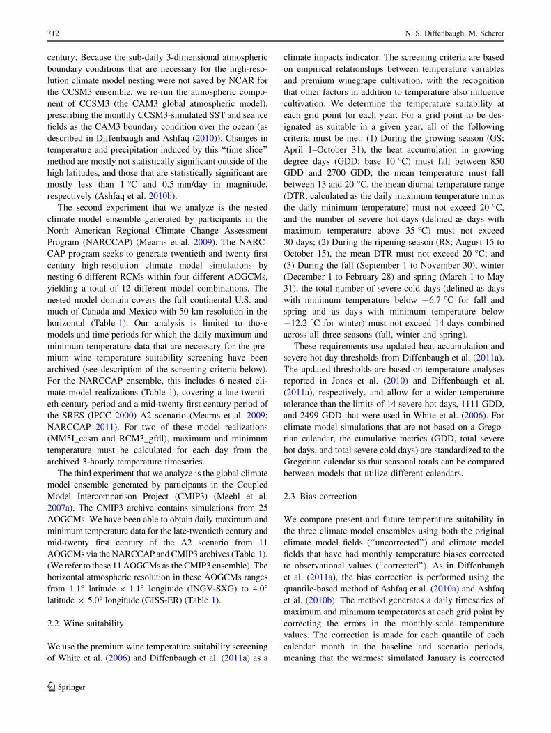
We analyze three ensemble climate model experiments

(Table 1). The first experiment is the high-resolution nested

climate model experiment generated by Diffenbaugh and

Ashfaq (2010), which we have extended to cover the period

from 1950 through 2099 in the SRES (IPCC 2000) A1B

scenario (Giorgi et al. 2011; Diffenbaugh et al. 2011b). The

ensemble consists of five realizations of the ICTP RegCM3

high-resolution climate model (Pal et al. 2007), each nested

within a different A1B realization of the NCAR CCSM3

global climate model (Collins et al. 2006) (Table 1). The

grid follows that of Diffenbaugh et al. (2005), covering the

full contiguous U.S. with 25-km resolution in the horizontal

and 18 levels in the vertical. The physics options also follow

those of Diffenbaugh et al. (2005), and are identical

between the five ensemble members. The five members are

thus physically uniform, but differ in the large-scale

boundary conditions provided by the respective CCSM3

realizations in which the RegCM3 realizations are nested.

The differences between the five CCSM3 realizations arise

from internal climate system variability, with the five

realizations initialized from different points in the CCSM3

pre-industrial control integration and then prescribed iden-

tical transient atmospheric constituent concentrations from

the mid-nineteenth century through the late-twenty first

Table 1 Climate model ensembles

Model realization Nested model Global model Resolution of atmosphere (km or degrees) Source

RegCM3 nested model ensemble (SRES A1B scenario)

RegCM3_bES RegCM3 ncar_ccsm3_0 25 D11a

RegCM3_c RegCM3 ncar_ccsm3_0 25 D11

RegCM3_e RegCM3 ncar_ccsm3_0 25 D11

RegCM3_fES RegCM3 ncar_ccsm3_0 25 D11

RegCM3_gES RegCM3 ncar_ccsm3_0 25 D11

NARCCAP nested model ensemble (SRES A2 scenario)

CRCM_cgcm3 CRCM cccma_cgcm3_1 50 NARCCAP

CRCM_ccsm CRCM ncar_ccsm3_0 50 NARCCAP

HRM3_hadcm3 HRM3 hadcm3 50 NARCCAP

MM5I_ccsm MM5I ncar_ccsm3_0 50 NARCCAP

RCM_gfdl RegCM3 gfdl_cm2_1 50 NARCCAP

WRFG_ccsm WRFG ncar_ccsm3_0 50 NARCCAP

CMIP3 global model ensemble (SRES A2 scenario)

GFDL-CM2.1 gfdl_cm2_1 2.0� 9 2.5� NARCCAP

CGCM3.1(T47) cccma_cgcm3_1 3.7� 9 3.8� NARCCAP

CNRM-CM3 cnrm_cm3 2.8� 9 2.8� PCMDI

CSIRO-Mk3.0 csiro_mk3_0 1.9� 9 1.9� PCMDI

CSIRO-Mk3.5 csiro_mk3_5 1.9� 9 1.9� PCMDI

GISS-ER giss_model_e_r 4.0� 9 5.0� PCMDI

INGV-SXG ingv_echam4 1.1� 9 1.1� PCMDI

IPSL-CM4 ipsl_cm4 2.5� 9 3.8� PCMDI

MIROC3.2(medres) miroc3_2_medres 2.8� 9 2.8� PCMDI

ECHO-G miub_echo_g 3.7� 9 3.8� PCMDI

ECHAM5/MPI-OM mpi_echam5 1.9� 9 1.9� PCMDI

a D11 = Diffenbaugh et al. (2011b)

Using climate impacts indicators to evaluate climate model ensembles 711

123

century. Because the sub-daily 3-dimensional atmospheric

boundary conditions that are necessary for the high-reso-

lution climate model nesting were not saved by NCAR for

the CCSM3 ensemble, we re-run the atmospheric compo-

nent of CCSM3 (the CAM3 global atmospheric model),

prescribing the monthly CCSM3-simulated SST and sea ice

fields as the CAM3 boundary condition over the ocean (as

described in Diffenbaugh and Ashfaq (2010)). Changes in

temperature and precipitation induced by this ‘‘time slice’’

method are mostly not statistically significant outside of the

high latitudes, and those that are statistically significant are

mostly less than 1 �C and 0.5 mm/day in magnitude,

respectively (Ashfaq et al. 2010b).

The second experiment that we analyze is the nested

climate model ensemble generated by participants in the

North American Regional Climate Change Assessment

Program (NARCCAP) (Mearns et al. 2009). The NARC-

CAP program seeks to generate twentieth and twenty first

century high-resolution climate model simulations by

nesting 6 different RCMs within four different AOGCMs,

yielding a total of 12 different model combinations. The

nested model domain covers the full continental U.S. and

much of Canada and Mexico with 50-km resolution in the

horizontal (Table 1). Our analysis is limited to those

models and time periods for which the daily maximum and

minimum temperature data that are necessary for the pre-

mium wine temperature suitability screening have been

archived (see description of the screening criteria below).

For the NARCCAP ensemble, this includes 6 nested cli-

mate model realizations (Table 1), covering a late-twenti-

eth century period and a mid-twenty first century period of

the SRES (IPCC 2000) A2 scenario (Mearns et al. 2009;

NARCCAP 2011). For two of these model realizations

(MM5I_ccsm and RCM3_gfdl), maximum and minimum

temperature must be calculated for each day from the

archived 3-hourly temperature timeseries.

The third experiment that we analyze is the global climate

model ensemble generated by participants in the Coupled

Model Intercomparison Project (CMIP3) (Meehl et al.

2007a). The CMIP3 archive contains simulations from 25

AOGCMs. We have been able to obtain daily maximum and

minimum temperature data for the late-twentieth century and

mid-twenty first century of the A2 scenario from 11

AOGCMs via the NARCCAP and CMIP3 archives (Table 1).

(We refer to these 11 AOGCMs as the CMIP3 ensemble). The

horizontal atmospheric resolution in these AOGCMs ranges

from 1.1� latitude 9 1.1� longitude (INGV-SXG) to 4.0�latitude 9 5.0� longitude (GISS-ER) (Table 1).

2.2 Wine suitability

We use the premium wine temperature suitability screening

of White et al. (2006) and Diffenbaugh et al. (2011a) as a

climate impacts indicator. The screening criteria are based

on empirical relationships between temperature variables

and premium winegrape cultivation, with the recognition

that other factors in addition to temperature also influence

cultivation. We determine the temperature suitability at

each grid point for each year. For a grid point to be des-

ignated as suitable in a given year, all of the following

criteria must be met: (1) During the growing season (GS;

April 1–October 31), the heat accumulation in growing

degree days (GDD; base 10 �C) must fall between 850

GDD and 2700 GDD, the mean temperature must fall

between 13 and 20 �C, the mean diurnal temperature range

(DTR; calculated as the daily maximum temperature minus

the daily minimum temperature) must not exceed 20 �C,

and the number of severe hot days (defined as days with

maximum temperature above 35 �C) must not exceed

30 days; (2) During the ripening season (RS; August 15 to

October 15), the mean DTR must not exceed 20 �C; and

(3) During the fall (September 1 to November 30), winter

(December 1 to February 28) and spring (March 1 to May

31), the total number of severe cold days (defined as days

with minimum temperature below -6.7 �C for fall and

spring and as days with minimum temperature below

-12.2 �C for winter) must not exceed 14 days combined

across all three seasons (fall, winter and spring).

These requirements use updated heat accumulation and

severe hot day thresholds from Diffenbaugh et al. (2011a).

The updated thresholds are based on temperature analyses

reported in Jones et al. (2010) and Diffenbaugh et al.

(2011a), respectively, and allow for a wider temperature

tolerance than the limits of 14 severe hot days, 1111 GDD,

and 2499 GDD that were used in White et al. (2006). For

climate model simulations that are not based on a Grego-

rian calendar, the cumulative metrics (GDD, total severe

hot days, and total severe cold days) are standardized to the

Gregorian calendar so that seasonal totals can be compared

between models that utilize different calendars.

2.3 Bias correction

We compare present and future temperature suitability in

the three climate model ensembles using both the original

climate model fields (‘‘uncorrected’’) and climate model

fields that have had monthly temperature biases corrected

to observational values (‘‘corrected’’). As in Diffenbaugh

et al. (2011a), the bias correction is performed using the

quantile-based method of Ashfaq et al. (2010a) and Ashfaq

et al. (2010b). The method generates a daily timeseries of

maximum and minimum temperatures at each grid point by

correcting the errors in the monthly-scale temperature

values. The correction is made for each quantile of each

calendar month in the baseline and scenario periods,

meaning that the warmest simulated January is corrected


123

by the error in the warmest simulated January, the second

warmest January is corrected by the error in the second

warmest January, and so on for all quantiles of each month

of the calendar. The method is thereby constructed to

preserve the simulated monthly- and daily-scale changes in

temperature at each grid point. As in Ashfaq et al. (2010a),

we perform the correction using the PRISM observational

monthly-mean daily maximum and minimum temperature

fields (Daly et al. 2000). Following both Ashfaq et al.

(2010a) and Diffenbaugh et al. (2011a), we first interpolate

the climate model and PRISM fields to a common 1/8th-

degree grid. Although the bias correction is performed at

the monthly scale, the baseline simulation of daily-scale

statistics is substantially improved by the correction

(Ashfaq et al. 2010a).

We compare the suitability screening in the three cli-

mate model ensembles with that in the NCEP North

American Regional Reanalysis (NARR) (Mesinger et al.

2006). The NARR reanalysis data are available with a

resolution of 32 km for the years 1979 through 2011. We

correct the biases in the NARR temperature fields using

the same approach as we use for the climate model

ensembles.

The quantile-based bias correction requires the time-

series to be of equal lengths in the baseline and scenario

periods. Our comparison of the climate model ensembles

and the reanalysis is therefore limited by the availability of

the different datasets. Based on the overlap of available

time period, we select 20 years to be our period of record.

Given the availability of the different datasets, we correct

the 20-year period from 1979 to 1998 in the NARR

reanalysis, and the 20-year periods from 1976 to 1995 and

2046 to 2065 in the three climate model ensembles.

Although the A2 and A1B emissions scenarios are not

identical over this period, the twenty first century cumu-

lative CO2 emissions are very similar in the two scenarios

[e.g., 731 and 893 GtC in 2050 and 2060, respectively, of

the A1B scenario and 729 and 912 GtC in 2050 and 2060,

respectively, of the A2 scenario (IPCC 2000)], and the

projected global warming over this mid-twentyfirst-century

period is indistinguishable (Meehl et al. 2007b).

As with the bias corrected datasets, all uncorrected

datasets are interpolated to a common 1/8th-degree grid

prior to analysis. In calculating the respective ensemble

means, we first calculate the temperature metrics for each

realization in the ensemble, and then calculate the mean of

the metrics across the realizations. In addition to compar-

ing the three climate model ensembles, we also create a

‘‘Superensemble’’ that includes projected mid-twenty first

century changes from all 22 realizations in the three cli-

mate model ensembles. This Superensemble allows us to

compare the mean and spread of the members of the

respective uncorrected and corrected ensembles with the

mean and spread of all members of all uncorrected and

corrected ensembles.

3 Results and discussion

3.1 Temperature suitability in the late-twentieth

century climate

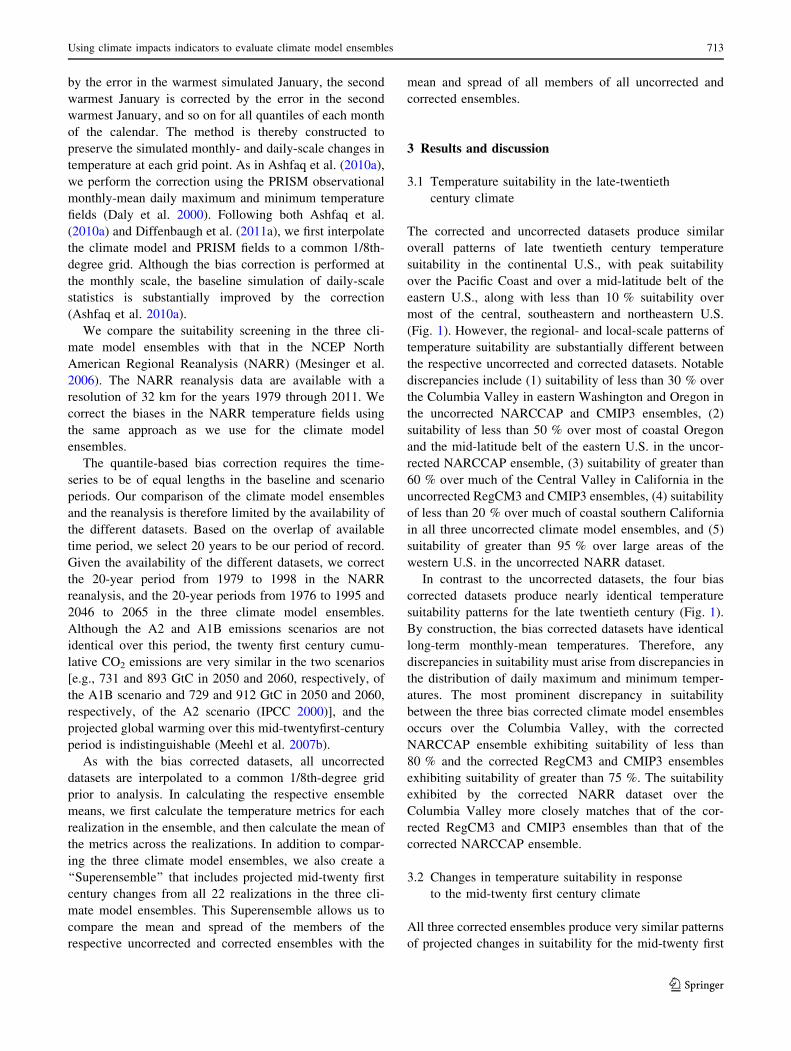
The corrected and uncorrected datasets produce similar

overall patterns of late twentieth century temperature

suitability in the continental U.S., with peak suitability

over the Pacific Coast and over a mid-latitude belt of the

eastern U.S., along with less than 10 % suitability over

most of the central, southeastern and northeastern U.S.

(Fig. 1). However, the regional- and local-scale patterns of

temperature suitability are substantially different between

the respective uncorrected and corrected datasets. Notable

discrepancies include (1) suitability of less than 30 % over

the Columbia Valley in eastern Washington and Oregon in

the uncorrected NARCCAP and CMIP3 ensembles, (2)

suitability of less than 50 % over most of coastal Oregon

and the mid-latitude belt of the eastern U.S. in the uncor-

rected NARCCAP ensemble, (3) suitability of greater than

60 % over much of the Central Valley in California in the

uncorrected RegCM3 and CMIP3 ensembles, (4) suitability

of less than 20 % over much of coastal southern California

in all three uncorrected climate model ensembles, and (5)

suitability of greater than 95 % over large areas of the

western U.S. in the uncorrected NARR dataset.

In contrast to the uncorrected datasets, the four bias

corrected datasets produce nearly identical temperature

suitability patterns for the late twentieth century (Fig. 1).

By construction, the bias corrected datasets have identical

long-term monthly-mean temperatures. Therefore, any

discrepancies in suitability must arise from discrepancies in

the distribution of daily maximum and minimum temper-

atures. The most prominent discrepancy in suitability

between the three bias corrected climate model ensembles

occurs over the Columbia Valley, with the corrected

NARCCAP ensemble exhibiting suitability of less than

80 % and the corrected RegCM3 and CMIP3 ensembles

exhibiting suitability of greater than 75 %. The suitability

exhibited by the corrected NARR dataset over the

Columbia Valley more closely matches that of the cor-

rected RegCM3 and CMIP3 ensembles than that of the

corrected NARCCAP ensemble.

3.2 Changes in temperature suitability in response

to the mid-twenty first century climate

All three corrected ensembles produce very similar patterns

of projected changes in suitability for the mid-twenty first


123

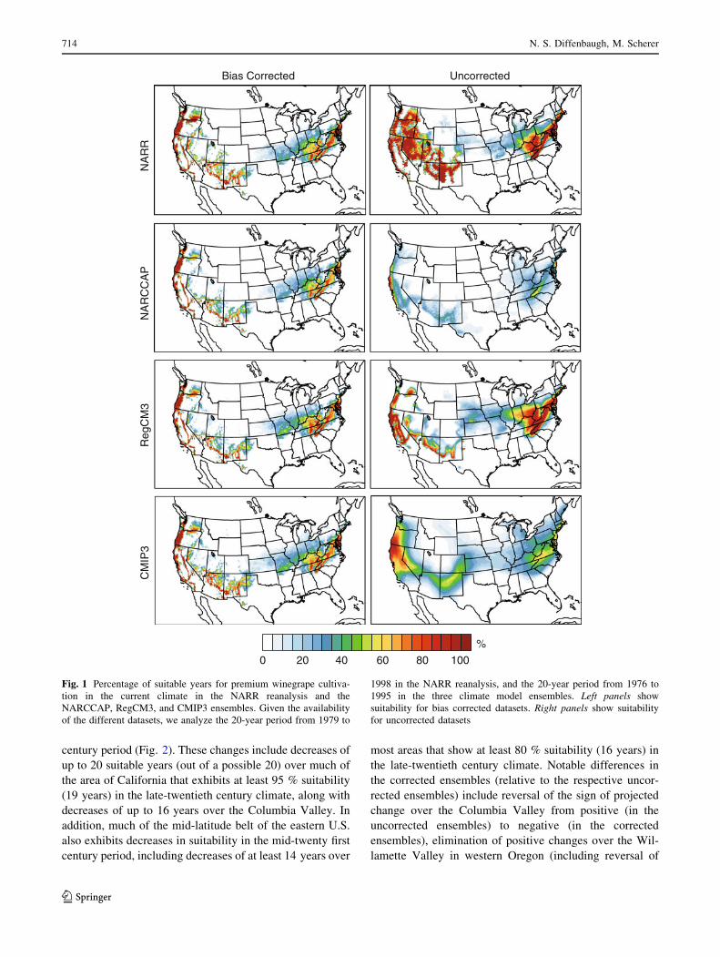
century period (Fig. 2). These changes include decreases of

up to 20 suitable years (out of a possible 20) over much of

the area of California that exhibits at least 95 % suitability

(19 years) in the late-twentieth century climate, along with

decreases of up to 16 years over the Columbia Valley. In

addition, much of the mid-latitude belt of the eastern U.S.

also exhibits decreases in suitability in the mid-twenty first

century period, including decreases of at least 14 years over

most areas that show at least 80 % suitability (16 years) in

the late-twentieth century climate. Notable differences in

the corrected ensembles (relative to the respective uncor-

rected ensembles) include reversal of the sign of projected

change over the Columbia Valley from positive (in the

uncorrected ensembles) to negative (in the corrected

ensembles), elimination of positive changes over the Wil-

lamette Valley in western Oregon (including reversal of

CM

IP3

Reg

CM

3N

AR

CC

AP

NA

RR

Bias Corrected Uncorrected

0 10020 40 60 80

%

Fig. 1 Percentage of suitable years for premium winegrape cultiva-

tion in the current climate in the NARR reanalysis and the

NARCCAP, RegCM3, and CMIP3 ensembles. Given the availability

of the different datasets, we analyze the 20-year period from 1979 to

1998 in the NARR reanalysis, and the 20-year period from 1976 to

1995 in the three climate model ensembles. Left panels show

suitability for bias corrected datasets. Right panels show suitability

for uncorrected datasets


123

sign in the NARCCAP ensemble), and reduction in the

spatial extent of negative changes over California.

Many of the largest projected future decreases in the

corrected ensembles occur over areas that currently repre-

sent important fractions of U.S. premium winegrape pro-

duction (Fig. 2) (Hodgen 2008). For example, the twenty

first century reductions in suitable years exceed 70 % of

the baseline suitable years over the northern and southern

Pacific coasts of California in all three corrected ensem-

bles, including at least 90 % reduction over the northern

Pacific coast in the NARCCAP and RegCM3 ensembles

and at least 90 % reduction over the southern Pacific coast

in the RegCM3 ensemble. Similarly, decreases over much

of the Columbia Valley exceed 50 % of the baseline suit-

able years in the NARCCAP and RegCM3 ensembles, and

exceed 40 % in the CMIP3 ensemble.


CM

IP3

Reg

CM

3N

AR

CC

AP

Sup

eren

sem

ble

0-10-20 10 20

years

Fig. 2 Change in suitable years for premium winegrape cultivation in

the NARCCAP, RegCM3, and CMIP3 ensembles, as well as the

combined Superensemble. Changes are calculated 2046–2065 minus

1976–1995. Positive changes reflect increasing suitability. Negative

changes reflect decreasing suitability. Left panels show suitability for

bias corrected datasets. Right panels show suitability for uncorrected

datasets


123

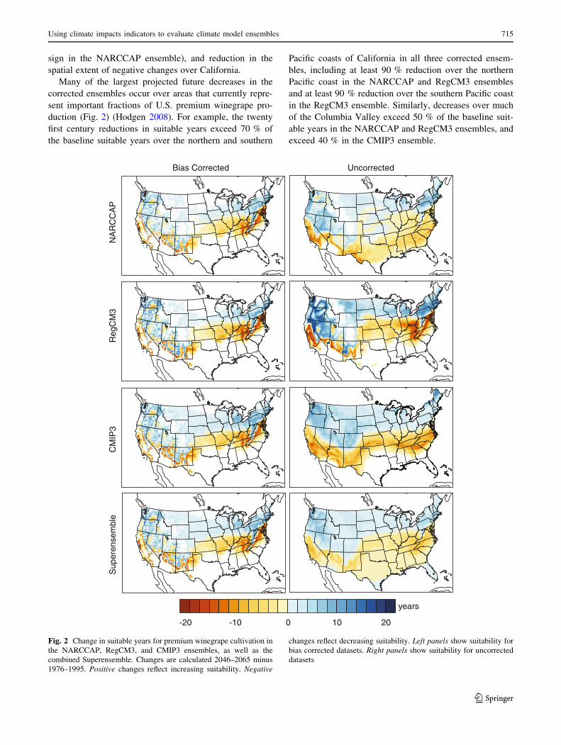
It is also notable that many of the largest projected

increases in suitable years occur over what are presently

the cool margins of temperature suitability. These include

widespread increases of at least 16 years (out of a possible

20) over higher-elevation areas of the western U.S. that are

adjacent to lower-elevation areas of high twentieth-century

suitability, and widespread increases of at least 8 years

over higher-latitude areas of the eastern U.S. that are

adjacent to lower-latitude areas of high twentieth-century

suitability (Fig. 1). These changes suggest a shift in

suitability upward in elevation and poleward in latitude as

cold limitation is removed in response to mid-twenty first

century warming.

3.3 Causes of mid-twenty first century changes

in temperature suitability

The projected mid-twenty first century decreases in overall

temperature suitability in the corrected ensembles are

associated with increases in the number of years in which

0-10-20 10 20

years

Severe Cold Days Severe Hot Days

Growing Season DTR Ripening Season DTR

Heat Accumulation Growing Season Temperature

Fig. 3 Change in the number of years in which the overall suitability

is limited by individual screening criteria in the bias corrected

Superensemble. Changes are calculated 2046–2065 minus

1976–1995. Positive changes reflect increasing limitation by an

individual criterion, and decreasing overall suitability. Negativechanges reflect decreasing limitation by an individual criterion, and

increasing overall suitability


123

the overall suitability is limited by the mean growing

season temperature and/or the number of severe hot days

(Fig. 3). For example, most areas of California that exhibit

decreases in overall suitability of at least 16 years in the

Superensemble also exhibit increases of at least 16 years in

limitation by mean growing season temperature (Figs. 2, 3).

In addition, areas of northern California that show

decreases in suitability of at least 16 years in the Supe-

rensemble also show increases of at least 14 years in lim-

itation by growing season hot days. Areas of the Columbia

Valley that exhibit decreases in overall suitability of at

least 8 years likewise exhibit increases of at least 10 years

in limitation by growing season hot days, while areas of the

eastern U.S. that show decreases in suitability of at least

12 years show increases of at least 16 years in limitation

by mean growing season temperature. The increase in the

number of years limited by an individual factor can be

greater than the decrease in total suitable years if other

individual criteria limit the baseline suitability. Indeed,

while large areas of the U.S. exhibit increases of at least

14 years in limitation by heat accumulation in the mid-

twenty first century period, the fact that other criteria limit

the late-twentieth century suitability to near-zero (Fig. 1)

causes the mid-twenty first century change in suitability

over those areas to also be near-zero (Fig. 2).

Areas of the western U.S. that show mid-twenty first

century increases in overall temperature suitability are

associated primarily with decreases in limitation by mean

growing season temperature and severe cold days (with

some areas also exhibiting decreased limitation by growing

season heat accumulation), while areas of the eastern U.S.

that show increased suitability are associated primarily with

decreases in limitation by severe cold days (Fig. 3). How-

ever, a number of high elevation areas of the western U.S.

and northerly areas of the eastern U.S. that exhibit decreases

in limitation by growing season heat accumulation and

mean growing season temperature in the bias corrected

ensembles also show no change in limitation by severe cold

days (Fig. 3). This continued limitation by severe cold days

during the twenty first century period limits the change in

overall temperature suitability over these areas, in spite of

increasing growing season suitability (Fig. 2).

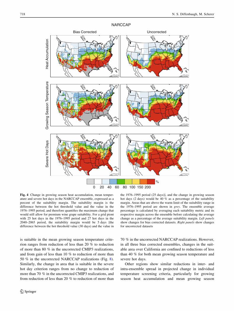
The climate model biases influence the projected twenty

first century change in temperature suitability by influ-

encing the ‘‘suitability margin’’, or the difference between

the threshold criterion value and the late-twentieth century

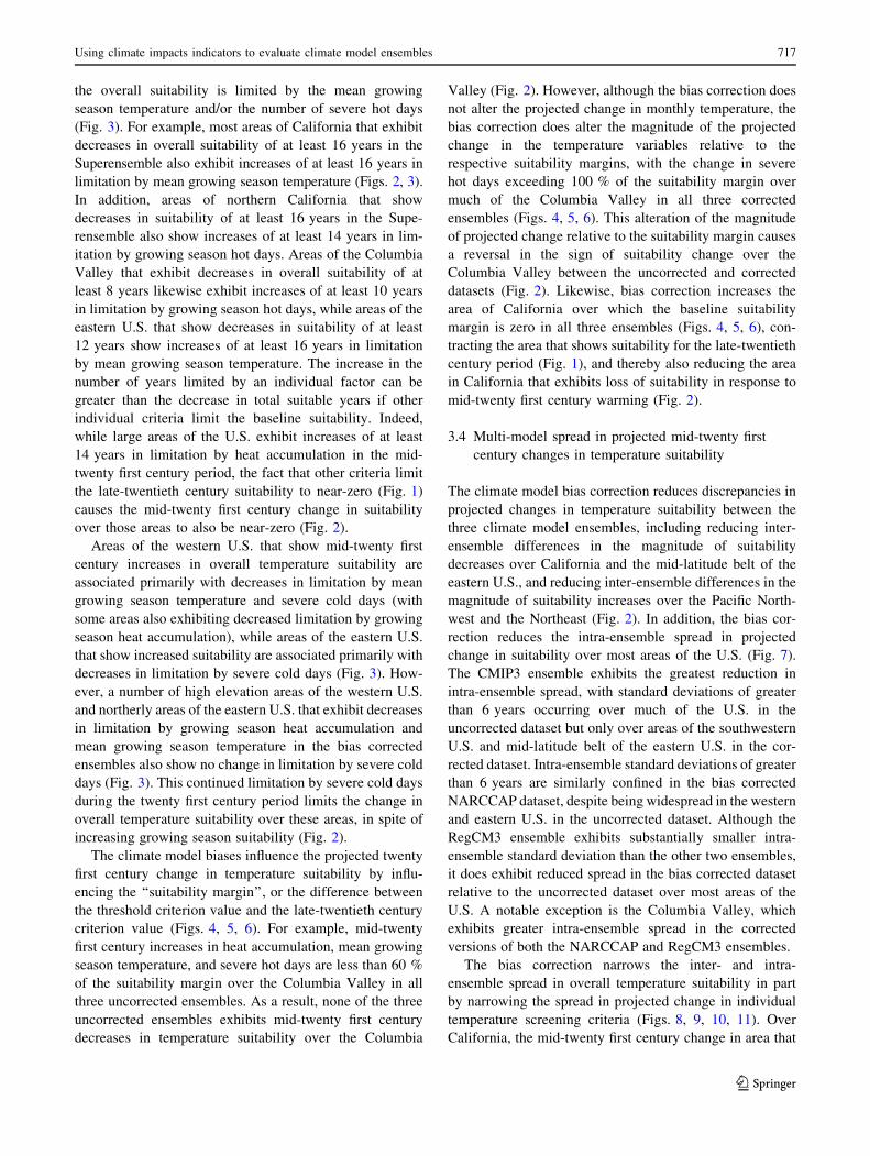
criterion value (Figs. 4, 5, 6). For example, mid-twenty

first century increases in heat accumulation, mean growing

season temperature, and severe hot days are less than 60 %

of the suitability margin over the Columbia Valley in all

three uncorrected ensembles. As a result, none of the three

uncorrected ensembles exhibits mid-twenty first century

decreases in temperature suitability over the Columbia

Valley (Fig. 2). However, although the bias correction does

not alter the projected change in monthly temperature, the

bias correction does alter the magnitude of the projected

change in the temperature variables relative to the

respective suitability margins, with the change in severe

hot days exceeding 100 % of the suitability margin over

much of the Columbia Valley in all three corrected

ensembles (Figs. 4, 5, 6). This alteration of the magnitude

of projected change relative to the suitability margin causes

a reversal in the sign of suitability change over the

Columbia Valley between the uncorrected and corrected

datasets (Fig. 2). Likewise, bias correction increases the

area of California over which the baseline suitability

margin is zero in all three ensembles (Figs. 4, 5, 6), con-

tracting the area that shows suitability for the late-twentieth

century period (Fig. 1), and thereby also reducing the area

in California that exhibits loss of suitability in response to

mid-twenty first century warming (Fig. 2).

3.4 Multi-model spread in projected mid-twenty first

century changes in temperature suitability

The climate model bias correction reduces discrepancies in

projected changes in temperature suitability between the

three climate model ensembles, including reducing inter-

ensemble differences in the magnitude of suitability

decreases over California and the mid-latitude belt of the

eastern U.S., and reducing inter-ensemble differences in the

magnitude of suitability increases over the Pacific North-

west and the Northeast (Fig. 2). In addition, the bias cor-

rection reduces the intra-ensemble spread in projected

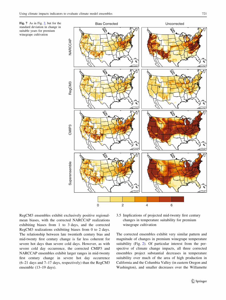
change in suitability over most areas of the U.S. (Fig. 7).

The CMIP3 ensemble exhibits the greatest reduction in

intra-ensemble spread, with standard deviations of greater

than 6 years occurring over much of the U.S. in the

uncorrected dataset but only over areas of the southwestern

U.S. and mid-latitude belt of the eastern U.S. in the cor-

rected dataset. Intra-ensemble standard deviations of greater

than 6 years are similarly confined in the bias corrected

NARCCAP dataset, despite being widespread in the western

and eastern U.S. in the uncorrected dataset. Although the

RegCM3 ensemble exhibits substantially smaller intra-

ensemble standard deviation than the other two ensembles,

it does exhibit reduced spread in the bias corrected dataset

relative to the uncorrected dataset over most areas of the

U.S. A notable exception is the Columbia Valley, which

exhibits greater intra-ensemble spread in the corrected

versions of both the NARCCAP and RegCM3 ensembles.

The bias correction narrows the inter- and intra-

ensemble spread in overall temperature suitability in part

by narrowing the spread in projected change in individual

temperature screening criteria (Figs. 8, 9, 10, 11). Over

California, the mid-twenty first century change in area that


123

is suitable in the mean growing season temperature crite-

rion ranges from reduction of less than 20 % to reduction

of more than 80 % in the uncorrected CMIP3 realizations,

and from gain of less than 10 % to reduction of more than

50 % in the uncorrected NARCCAP realizations (Fig. 8).

Similarly, the change in area that is suitable in the severe

hot day criterion ranges from no change to reduction of

more than 70 % in the uncorrected CMIP3 realizations, and

from reduction of less than 20 % to reduction of more than

70 % in the uncorrected NARCCAP realizations. However,

in all three bias corrected ensembles, changes in the suit-

able area over California are confined to reductions of less

than 40 % for both mean growing season temperature and

severe hot days.

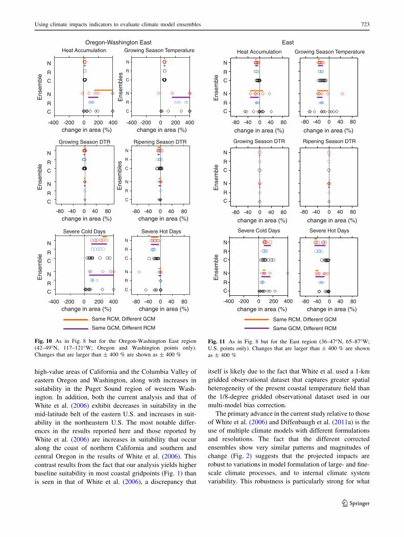
Other regions show similar reductions in inter- and

intra-ensemble spread in projected change in individual

temperature screening criteria, particularly for growing

season heat accumulation and mean growing season

NARCCAP

Sev

ere

Hot

Day

sH

eat A

ccum

ulat

ion

Gro

win

g S

easo

n Te

mpe

ratu

re


0 20 8040 60 100 150 200

%

Fig. 4 Change in growing season heat accumulation, mean temper-

ature and severe hot days in the NARCCAP ensemble, expressed as a

percent of the suitability margin. The suitability margin is the

difference between the hot threshold value and the value in the

1976–1995 period, and therefore quantifies the maximum change that

would still allow for premium wine grape suitability. For a grid piont

with 25 hot days in the 1976–1995 period and 27 hot days in the

2040–2065 period, the suitability margin would be 5 days [the

difference between the hot threshold value (30 days) and the value in

the 1976–1995 period (25 days)], and the change in growing season

hot days (2 days) would be 40 % as a percentage of the suitability

margin. Areas that are above the warm limit of the suitability range in

the 1976–1995 period are shown in grey. The ensemble average

percentage is calculated by averaging each suitability metric and its

respective margin across the ensemble before calculating the average

change as a percentage of the average suitability margin. Left panelsshow changes for bias corrected datasets. Right panels show changes

for uncorrected datasets


123

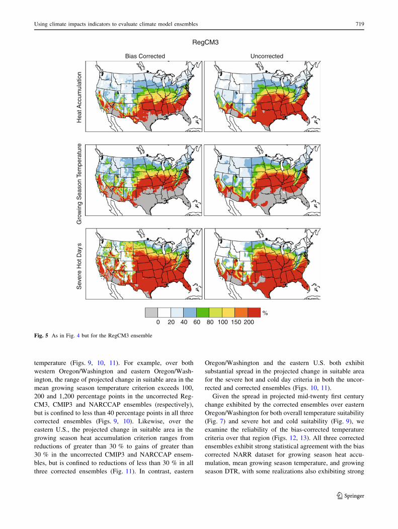
temperature (Figs. 9, 10, 11). For example, over both

western Oregon/Washington and eastern Oregon/Wash-

ington, the range of projected change in suitable area in the

mean growing season temperature criterion exceeds 100,

200 and 1,200 percentage points in the uncorrected Reg-

CM3, CMIP3 and NARCCAP ensembles (respectively),

but is confined to less than 40 percentage points in all three

corrected ensembles (Figs. 9, 10). Likewise, over the

eastern U.S., the projected change in suitable area in the

growing season heat accumulation criterion ranges from

reductions of greater than 30 % to gains of greater than

30 % in the uncorrected CMIP3 and NARCCAP ensem-

bles, but is confined to reductions of less than 30 % in all

three corrected ensembles (Fig. 11). In contrast, eastern

Oregon/Washington and the eastern U.S. both exhibit

substantial spread in the projected change in suitable area

for the severe hot and cold day criteria in both the uncor-

rected and corrected ensembles (Figs. 10, 11).

Given the spread in projected mid-twenty first century

change exhibited by the corrected ensembles over eastern

Oregon/Washington for both overall temperature suitability

(Fig. 7) and severe hot and cold suitability (Fig. 9), we

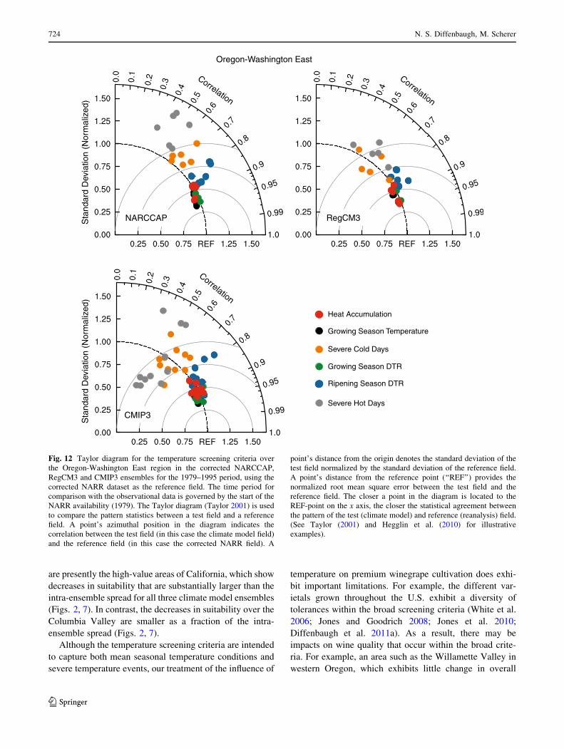
examine the reliability of the bias-corrected temperature

criteria over that region (Figs. 12, 13). All three corrected

ensembles exhibit strong statistical agreement with the bias

corrected NARR dataset for growing season heat accu-

mulation, mean growing season temperature, and growing

season DTR, with some realizations also exhibiting strong

RegCM3

Sev

ere

Hot

Day

sH

eat A

ccum

ulat

ion

Gro

win

g S

easo

n Te

mpe

ratu

re


0 20 8040 60 100 150 200

%

Fig. 5 As in Fig. 4 but for the RegCM3 ensemble


123

agreement for ripening season DTR (Fig. 12). However, all

three corrected ensembles show considerably weaker

agreement for severe hot and cold day occurrence, with the

NARCCAP- and CMIP3-simulated severe cold day values

showing the weakest agreement with the corrected NARR

dataset.

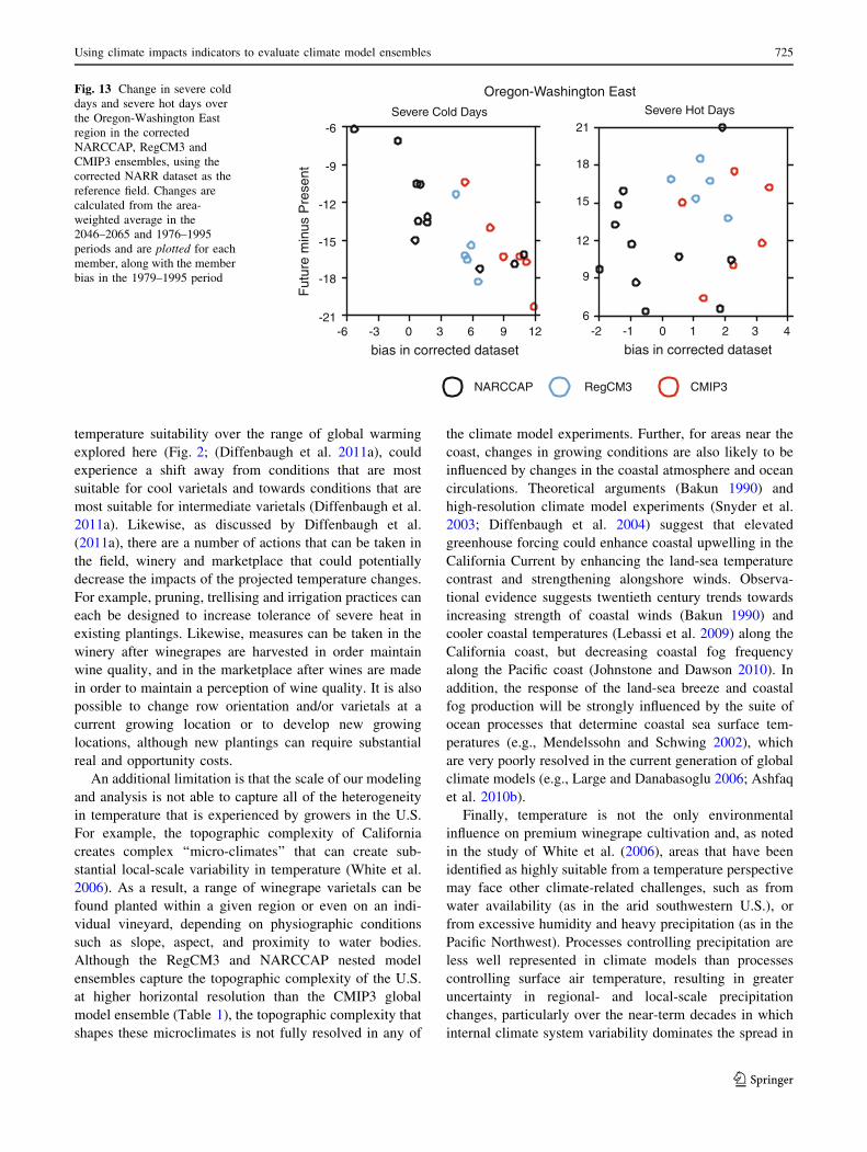
The regional-mean severe cold day bias ranges from -5

to 11 days over eastern Oregon-Washington in the cor-

rected CMIP3 ensemble (Fig. 13). The smaller NARCCAP

and RegCM3 ensembles exhibit exclusively positive

regional-mean biases, with the corrected NARCCAP real-

izations exhibiting biases from 5 to 11 days, and the cor-

rected RegCM3 realizations exhibiting biases from 4 to

7 days. In all three corrected ensembles, the most negative

severe cold day biases are associated with the least

negative mid-twenty first century changes in severe cold

day occurrence, while the most positive severe cold day

biases are associated with the most negative mid-twenty

first century changes. This relationship could be expected

given that the number of severe cold days is zero-bounded,

and that the projected mid-twenty first century period is

warmer than the late-twentieth century period: for a

reduction in severe cold day occurrence in response to

mean warming, negative biases artificially decrease the

reduction in severe cold days that is possible before

reaching zero, while positive biases artificially increase the

reduction that is possible.

The regional-mean severe hot day bias ranges from -2

to 2 days in the corrected CMIP3 ensemble (Fig. 13). As

with the severe cold day bias, the smaller NARCCAP and

CMIP3

Sev

ere

Hot

Day

sH

eat A

ccum

ulat

ion

Gro

win

g S

easo

n Te

mpe

ratu

re


0 20 8040 60 100 150 200

%

Fig. 6 As in Fig. 5 but for the CMIP3 ensemble


123

RegCM3 ensembles exhibit exclusively positive regional-

mean biases, with the corrected NARCCAP realizations

exhibiting biases from 1 to 3 days, and the corrected

RegCM3 realizations exhibiting biases from 0 to 2 days.

The relationship between late twentieth century bias and

mid-twenty first century change is far less coherent for

severe hot days than severe cold days. However, as with

severe cold day occurrence, the corrected CMIP3 and

NARCCAP ensembles exhibit larger ranges in mid-twenty

first century change in severe hot day occurrence

(6–21 days and 7–17 days, respectively) than the RegCM3

ensemble (13–19 days).

3.5 Implications of projected mid-twenty first century

changes in temperature suitability for premium

winegrape cultivation

The corrected ensembles exhibit very similar pattern and

magnitude of changes in premium winegrape temperature

suitability (Fig. 2). Of particular interest from the per-

spective of climate change impacts, all three corrected

ensembles project substantial decreases in temperature

suitability over much of the area of high production in

California and the Columbia Valley (in eastern Oregon and

Washington), and smaller decreases over the Willamette


CM

IP3

Reg

CM

3N

AR

CC

AP

Sup

eren

sem

ble

0 2 4 6

Fig. 7 As in Fig. 2, but for the

standard deviation in change in

suitable years for premium

winegrape cultivation


123

Valley (in western Oregon). These decreases in suitability

are primarily associated with increases in excessive mean

growing season temperature and excessive occurrence of

growing season severe hot days. In addition, projected

increases in suitable years in the corrected ensembles are

concentrated in areas that do not currently exhibit high

temperature suitability.

The results are broadly similar to those reported by

White et al. (2006) analyzing a single model, single real-

ization climate model experiment for the late-twenty first

century in the A2 scenario, and those reported by Dif-

fenbaugh et al. (2011a) analyzing a single model, multiple

realization climate model experiment for the early-twenty

first century in the A1B scenario. For example, all three

studies report substantial decreases in suitability in the

California




change in area (%) change in area (%)


change in area (%) change in area (%)0 40 80-40-800 40 80-40-80

Ens

embl

e

N

R

C

N

R

C

Ens

embl

e

N

R

C

N

R

C

Ens

embl

e

N

R

C

N

R

C

-80 0 40 80-40

Same RCM, Different GCM

Same GCM, Different RCM

-80 0 40 80-40

-80 0 40 80-40-80 0 40 80-40

Fig. 8 The projected change in area that is suitable in each of the

temperature screening criteria in the California region (34–42�N,

118–125�W; California points only). Each realization is shown from

the NARCCAP (N), RegCM3 (R) and CMIP3 (C) ensembles.

Changes are calculated 2046–2065 minus 1976–1995, and are

presented as area normalized to the total area of the region in

percentage. Circles denote bias corrected data and diamonds denote

uncorrected data. Red symbols denote the NARCCAP ensemble, bluesymbols denote the RegCM3 ensemble, and black symbols denote the

CMIP3 ensemble. The orange bars show the range of values for the

NARCCAP realizations that use the same nested climate model but

different global climate models. The purple bars show the range of

values for the NARCCAP realizations that use the same global

climate model but different nested climate models

Oregon-Washington West






change in area (%) change in area (%)0 200 400-200-4000 200 400-200-400

Ens

embl

e

N

R

C

N

R

C

Ens

embl

e

N

R

C

N

R

CE

nsem

ble

N

R

C

N

R

C

0 40 80-40-80 0 40 80-40-80



0 40 80-40-800 40 80-40-80

Fig. 9 As in Fig. 8 but for the Oregon-Washington West region

(42–49�N, 121–25�W; Oregon and Washington points only). Changes

that are larger than ±400 % are shown as ±400 %


123

high-value areas of California and the Columbia Valley of

eastern Oregon and Washington, along with increases in

suitability in the Puget Sound region of western Wash-

ington. In addition, both the current analysis and that of

White et al. (2006) exhibit decreases in suitability in the

mid-latitude belt of the eastern U.S. and increases in suit-

ability in the northeastern U.S. The most notable differ-

ences in the results reported here and those reported by

White et al. (2006) are increases in suitability that occur

along the coast of northern California and southern and

central Oregon in the results of White et al. (2006). This

contrast results from the fact that our analysis yields higher

baseline suitability in most coastal gridpoints (Fig. 1) than

is seen in that of White et al. (2006), a discrepancy that

itself is likely due to the fact that White et al. used a 1-km

gridded observational dataset that captures greater spatial

heterogeneity of the present coastal temperature field than

the 1/8-degree gridded observational dataset used in our

multi-model bias correction.

The primary advance in the current study relative to those

of White et al. (2006) and Diffenbaugh et al. (2011a) is the

use of multiple climate models with different formulations

and resolutions. The fact that the different corrected

ensembles show very similar patterns and magnitudes of

change (Fig. 2) suggests that the projected impacts are

robust to variations in model formulation of large- and fine-

scale climate processes, and to internal climate system

variability. This robustness is particularly strong for what

Oregon-Washington East







Ens

embl

e

Ens

embl

es

N

R

C

N

R

C

Ens

embl

e

N

R

C

N

R

C

Ens

embl

e

N

R

C

N

R

C

0 200 400-200-4000 200 400-200-400

0 200 400-200-400

0 40 80-40-80



Ens

embl

es

0 40 80-40-80

0 40 80-40-80

Fig. 10 As in Fig. 8 but for the Oregon-Washington East region

(42–49�N, 117–121�W; Oregon and Washington points only).

Changes that are larger than ± 400 % are shown as ± 400 %

East







Ens

embl

e

N

R

C

N

R

C

Ens

embl

e

N

R

C

N

R

C

Ens

embl

e

N

R

C

N

R

C

0 40 80-40-80

0 200 400-200-400



0 40 80-40-80

0 40 80-40-80

0 40 80-40-80

0 40 80-40-80

Fig. 11 As in Fig. 8 but for the East region (36–47�N, 65–87�W;

U.S. points only). Changes that are larger than ± 400 % are shown

as ± 400 %


123

are presently the high-value areas of California, which show

decreases in suitability that are substantially larger than the

intra-ensemble spread for all three climate model ensembles

(Figs. 2, 7). In contrast, the decreases in suitability over the

Columbia Valley are smaller as a fraction of the intra-

ensemble spread (Figs. 2, 7).

Although the temperature screening criteria are intended

to capture both mean seasonal temperature conditions and

severe temperature events, our treatment of the influence of

temperature on premium winegrape cultivation does exhi-

bit important limitations. For example, the different var-

ietals grown throughout the U.S. exhibit a diversity of

tolerances within the broad screening criteria (White et al.

2006; Jones and Goodrich 2008; Jones et al. 2010;

Diffenbaugh et al. 2011a). As a result, there may be

impacts on wine quality that occur within the broad crite-

ria. For example, an area such as the Willamette Valley in

western Oregon, which exhibits little change in overall

Severe Cold Days

Severe Hot Days

Growing Season DTR

Ripening Season DTR

Heat Accumulation

Growing Season Temperature


Correlation

Correlation

Correlation

Sta

ndar

d D

evia

tion

(Nor

mal

ized

)S

tand

ard

Dev

iatio

n (N

orm

aliz

ed)

NARCCAP RegCM3

CMIP3

Fig. 12 Taylor diagram for the temperature screening criteria over

the Oregon-Washington East region in the corrected NARCCAP,

RegCM3 and CMIP3 ensembles for the 1979–1995 period, using the

corrected NARR dataset as the reference field. The time period for

comparison with the observational data is governed by the start of the

NARR availability (1979). The Taylor diagram (Taylor 2001) is used

to compare the pattern statistics between a test field and a reference

field. A point’s azimuthal position in the diagram indicates the

correlation between the test field (in this case the climate model field)

and the reference field (in this case the corrected NARR field). A

point’s distance from the origin denotes the standard deviation of the

test field normalized by the standard deviation of the reference field.

A point’s distance from the reference point (‘‘REF’’) provides the

normalized root mean square error between the test field and the

reference field. The closer a point in the diagram is located to the

REF-point on the x axis, the closer the statistical agreement between

the pattern of the test (climate model) and reference (reanalysis) field.

(See Taylor (2001) and Hegglin et al. (2010) for illustrative

examples).


123

temperature suitability over the range of global warming

explored here (Fig. 2; (Diffenbaugh et al. 2011a), could

experience a shift away from conditions that are most

suitable for cool varietals and towards conditions that are

most suitable for intermediate varietals (Diffenbaugh et al.

2011a). Likewise, as discussed by Diffenbaugh et al.

(2011a), there are a number of actions that can be taken in

the field, winery and marketplace that could potentially

decrease the impacts of the projected temperature changes.

For example, pruning, trellising and irrigation practices can

each be designed to increase tolerance of severe heat in

existing plantings. Likewise, measures can be taken in the

winery after winegrapes are harvested in order maintain

wine quality, and in the marketplace after wines are made

in order to maintain a perception of wine quality. It is also

possible to change row orientation and/or varietals at a

current growing location or to develop new growing

locations, although new plantings can require substantial

real and opportunity costs.

An additional limitation is that the scale of our modeling

and analysis is not able to capture all of the heterogeneity

in temperature that is experienced by growers in the U.S.

For example, the topographic complexity of California

creates complex ‘‘micro-climates’’ that can create sub-

stantial local-scale variability in temperature (White et al.

2006). As a result, a range of winegrape varietals can be

found planted within a given region or even on an indi-

vidual vineyard, depending on physiographic conditions

such as slope, aspect, and proximity to water bodies.

Although the RegCM3 and NARCCAP nested model

ensembles capture the topographic complexity of the U.S.

at higher horizontal resolution than the CMIP3 global

model ensemble (Table 1), the topographic complexity that

shapes these microclimates is not fully resolved in any of

the climate model experiments. Further, for areas near the

coast, changes in growing conditions are also likely to be

influenced by changes in the coastal atmosphere and ocean

circulations. Theoretical arguments (Bakun 1990) and

high-resolution climate model experiments (Snyder et al.

2003; Diffenbaugh et al. 2004) suggest that elevated

greenhouse forcing could enhance coastal upwelling in the

California Current by enhancing the land-sea temperature

contrast and strengthening alongshore winds. Observa-

tional evidence suggests twentieth century trends towards

increasing strength of coastal winds (Bakun 1990) and

cooler coastal temperatures (Lebassi et al. 2009) along the

California coast, but decreasing coastal fog frequency

along the Pacific coast (Johnstone and Dawson 2010). In

addition, the response of the land-sea breeze and coastal

fog production will be strongly influenced by the suite of

ocean processes that determine coastal sea surface tem-

peratures (e.g., Mendelssohn and Schwing 2002), which

are very poorly resolved in the current generation of global

climate models (e.g., Large and Danabasoglu 2006; Ashfaq

et al. 2010b).

Finally, temperature is not the only environmental

influence on premium winegrape cultivation and, as noted

in the study of White et al. (2006), areas that have been

identified as highly suitable from a temperature perspective

may face other climate-related challenges, such as from

water availability (as in the arid southwestern U.S.), or

from excessive humidity and heavy precipitation (as in the

Pacific Northwest). Processes controlling precipitation are

less well represented in climate models than processes

controlling surface air temperature, resulting in greater

uncertainty in regional- and local-scale precipitation

changes, particularly over the near-term decades in which

internal climate system variability dominates the spread in

Severe Hot DaysSevere Cold Days

bias in corrected dataset-6 -3 0 3 6 9 12 10-1-2 2 3 4

6

9

12

15

18

21-6

-9

-12

-15

-18

-21F

utur

e m

inus

Pre

sent

NARCCAP RegCM3 CMIP3


bias in corrected dataset

Fig. 13 Change in severe cold

days and severe hot days over

the Oregon-Washington East

region in the corrected

NARCCAP, RegCM3 and

CMIP3 ensembles, using the

corrected NARR dataset as the

reference field. Changes are

calculated from the area-

weighted average in the

2046–2065 and 1976–1995

periods and are plotted for each

member, along with the member

bias in the 1979–1995 period


123

climate model projections of precipitation over the western

U.S. (Hawkins and Sutton 2010). However, given that

much of the water consumed for agriculture in the western

U.S. is delivered and stored as snowpack (Mock 1996;

Hamlet and Lettenmaier 1999), the prospect of tempera-

ture-driven shifts towards decreased snow-to-precipitation

ratio and earlier snowmelt timing (Leung and Ghan 1999;

Hamlet et al. 2005; Maurer and Duffy 2005; Mote et al.

2005; Maurer 2007; Rauscher et al. 2008) suggests that

premium winegrape cultivation may require increasing

tolerance of severe heat and decreased water availability in

the coming decades.

4 Conclusions

Our results suggest that global warming that is projected to

occur by the mid-twenty first century could substantially

displace the geographic distribution of optimal temperature

conditions for the cultivation of premium winegrapes, with

the areas that currently account for most of the U.S. pro-

duction experiencing growing conditions that are substan-

tially warmer than present, and the optimal temperature

conditions in the future occurring in areas that are currently

at the cool margin of premium winegrape suitability.

Although previous research has suggested similar wine-

grape impacts using single-model climate modeling

frameworks (e.g., White et al. 2006; Diffenbaugh et al.

2011a), this is the first such national-scale analysis using a

multi-model ensemble approach. The agreement between

those previous studies and the multi-model analysis pre-

sented here suggests that the previously reported results are

robust.

Comparing the spread within and between different

climate model ensembles can help to constrain the mag-

nitude of different sources of uncertainty in future climate

change (e.g., Deque et al. 2005; Giorgi et al. 2008;

Hawkins and Sutton 2009, 2010). Like most multi-model

ensembles created to date, the three ensembles analyzed

here are not perfectly uniform in their experimental design

(e.g., Table 1). However, despite the fact that they do not

form a perfect experiment, some insight about climate

change uncertainty can be drawn from comparing the intra-

and inter-ensemble variations.

For example, comparison of the three ensembles shows

that the RegCM3 ensemble exhibits the smallest intra-

ensemble spread in the impact of mid-twenty first century

climate change on premium winegrape temperature suit-

ability (Figs. 7, 8, 9, 10, 11). Because the five RegCM3

realizations are physically uniform, this result suggests

that—for the temperature suitability examined here—the

uncertainty arising from internal climate system variability

is smaller than the uncertainty arising from climate model

formulation. In addition, the 6-member NARCCAP

ensemble and the 11-member CMIP3 ensemble exhibit

similar mid-twenty first century intra-ensemble spread over

the regions of high temperature suitability (Figs. 7, 8, 9, 10,

11). Further, in most cases, the range between realizations

using the same nested model but different AOGCMs is

equal to or less than the range between realizations using

different nested models but the same AOGCM (Figs. 8, 9,

10, 11). Although the population size is small (the 6

NARCCAP realizations are nested within only 4 AOGCM

realizations; Table 1), these results suggest that the

uncertainty arising from the model formulation of fine-

scale climate processes is not smaller than the uncertainty

arising from the model formulation of large-scale climate

processes.

Comparison of the three ensembles also shows that bias

correction reduces the inter-ensemble spread, along with

the intra-ensemble spread within the NARCCAP and

CMIP3 ensembles (Figs 2, 7, 8, 9, 10, 11). These results

suggest that the climate model biases dominate the multi-

model spread, particularly through the suitability margin

between baseline temperature values and critical tempera-

ture thresholds (Figs. 4, 6). The fact that climate model

biases have been found not to dominate the multi-model

regional temperature change (Giorgi and Coppola 2011)

highlights the importance of using climate impacts indi-

cators to evaluate the spread in climate model ensembles,

as the simulated climate change and the simulated climate

change impacts may show different sensitivities to model

biases.

Identification and quantification of the importance of

climate model biases is certainly not new. Indeed, the

importance of bias correction has long been recognized in

the climate modeling community, and is used particularly

prominently in hydrologic impacts work (e.g., Maurer and

Duffy 2005; Maurer 2007) and seasonal climate prediction

(e.g., Landman and Goddard 2002; Baigorria et al. 2007).

What has received less attention is the importance of cli-

mate model biases in shaping the model agreement in

simulated climate change impacts. In our approach, the

simulated monthly-scale temperature change between the

present and future periods is preserved in each model

realization. As a result, the model differences in simulated

temperature change are also preserved. These model dif-

ferences can be substantial, and understanding the causes

of such differences has received considerable attention in

the literature (e.g., Meehl et al. 2007b). However, to the

best of our knowledge, this is the first attempt to system-

atically evaluate the contributions of intra-model variabil-

ity, inter-model differences, and climate model bias to the

spread in the simulated impacts of climate change. The fact

that the corrected ensembles show very similar results over

most of the U.S. even though the model differences in the


123

simulated temperature changes are preserved suggests

that—at least for some systems—the projected climate

change impacts could be more robust than the projected

climate change.

In addition, the fact that some areas do show substantial

variation between the corrected ensembles helps to identify

sources of particular uncertainty in future climate change

impacts. In our analyses, variations in the corrected

ensembles are seen most prominently in areas where errors

in the temperature extremes persist after bias correction,

such as for severe hot and cold days over eastern Oregon-

Washington (Figs. 12, 13). These errors further highlight

the importance of continued efforts to improve the climate

model representation of extreme events. Specifically, the

fact that the three corrected climate model ensembles have

identical mean monthly temperature values in the baseline

period but exhibit substantial variation in the occurrence of

extreme hot and cold events suggests that the processes that

dictate daily temperature variability require further under-

standing. This is likely to also be a prominent need for

precipitation, as changes in the extremes of precipitation

are not always linearly correlated with changes in the mean

of the precipitation distribution (e.g., Wehner 2004).

It is important to consider that this study examines only

one impacts indicator for one human system, and that this

indicator is based only on surface air temperature.

Although the cultivation of premium winegrapes exhibits

well-developed relationships with temperature, the contri-

bution of different sources of uncertainty to the overall

spread in the response to enhanced radiative forcing is

likely to vary between climate-sensitive systems. While it

is clearly not feasible to conduct a case study of every

conceivable climate-sensitive system, our finding that cli-

mate model bias dominates the spread in projected climate

change impact should be tested across a range of impacts

indicators. By increasing the focus on the climate phe-

nomena that most directly influence natural and human

systems, extension of this analysis to a larger suite of

impacts indicators will help to deepen our understanding of

the mechanisms and uncertainty of future climate change.

Acknowledgments We thank two anonymous reviewers for

insightful and constructive comments. We wish to thank the North

American Regional Climate Change Assessment Program (NARC-

CAP) for providing the NARCCAP data used in this paper. NARC-

CAP is funded by the National Science Foundation (NSF), the U.S.

Department of Energy (DoE), the National Oceanic and Atmospheric

Administration (NOAA), and the U.S. Environmental Protection

Agency Office of Research and Development (EPA). We acknowl-

edge the modeling groups, the Program for Climate Model Diagnosis

and Intercomparison (PCMDI) and the WCRP’s Working Group on

Coupled Modelling (WGCM) for their roles in making available the

WCRP CMIP3 multi-model dataset. Support of the CMIP3 dataset is

provided by the Office of Science, U.S. Department of Energy. We

thank the National Centers for Environmental Prediction (NCEP) for

providing access to the North American Regional Reanalysis (NARR)

dataset, and the PRISM Climate Group and Oregon State University

for providing access to the PRISM observational temperature dataset.

Our RegCM3 climate model experiments were generated and stored

using computing resources provided by the Rosen Center for

Advanced Computing (RCAC) at Purdue University, and our analyses

of all datasets were performed using computing resources provided

by the Center for Computational Earth and Environmental Sci-

ence (CEES) at Stanford University. The research reported

here was supported by NSF award 0955283 and NIH award

1R01AI090159-01.

References

Adger WN, Brooks N, et al. (2004) New indicators of vulnerability

and adaptive capacity. Technical report 7. Norwich, U.K.,

Tyndall Centre for Climate Change Research

Ahmed SA, Diffenbaugh NS, et al. (2009) Climate volatility deepens

poverty vulnerability in developing countries. Environ Res Lett

4(3):034004. doi:10.1088/1748-9326/4/3/034004

Ahmed SA, Diffenbaugh NS, et al. (2010) Climate volatility and

poverty vulnerability in Tanzania. Global Environ Change. doi:

10.1016/j.gloenvcha.2010.1010.1003

Annamalai H, Hamilton K et al (2007) The South Asian summer

monsoon and its relationship with ENSO in the IPCC AR4

simulations. J Clim 20(6):1071–1092

Ashfaq M, Bowling LC, et al. (2010a). Influence of climate model

biases and daily-scale temperature and precipitation events on

hydrological impacts assessment: a case study of the United

States. J Geophys Res 115:D14116. doi:14110.11029/12009JD

012965

Ashfaq M, Skinner CB, et al. (2010b). Influence of SST biases on

future climate change projections. Climate Dynam. doi:10.1007/

s00382-00010-00875-00382

Baigorria GA, Jones JW et al (2007) Assessing uncertainties in crop

model simulations using daily bias-corrected regional circulation

model outputs. Climate Res 34(3):211–222

Bakun A (1990) Global climate change and intensification of coastal

ocean upwelling. Science 247(4939):198–201

Christensen JH, Christensen OB (2003) Climate modelling: severe

summertime flooding in Europe. Nature 421(6925):805–806

Christensen JH, Hewitson B, et al. (2007) Regional climate projec-

tions. Climate change 2007: the physical science basis. Contri-

bution of working group I to the fourth assessment report of the

intergovernmental panel on climate change. Solomon S, Qin D,

Manning M, et al. Cambridge, United Kingdom and New York,

NY, USA, Cambridge University Press

Collins WD, Bitz CM et al (2006) The community climate system

model version 3 (CCSM3). J Clim 19(11):2122–2143

Daly C, Taylor GH et al (2000) High-quality spatial climate data sets

for the United States and beyond. Transactions of the ASAE

43(6):1957–1962

Deque M, Jones RG et al (2005) Global high resolution versus limited

area model climate change projections over Europe: quantifying

confidence level from PRUDENCE results. Clim Dyn 25(6):

653–670

Diffenbaugh NS, Ashfaq M (2010) Intensification of hot extremes in

the United States. Geophys Res Lett 37:L15701. doi:15710.

11029/12010GL043888

Diffenbaugh NS, Snyder MA et al (2004) Could CO2-induced land

cover feedbacks alter near-shore upwelling regimes? Proc Nat

Acad Sci 101(1):27–32

Diffenbaugh NS, Pal JS et al (2005) Fine-scale processes regulate the

response of extreme events to global climate change. Proc Nat

Acad Sci USA 102(44):15774–15778


123

http://dx.doi.org/10.1088/1748-9326/4/3/034004

http://dx.doi.org/10.1016/j.gloenvcha.2010.1010.1003

http://dx.doi.org/14110.11029/12009JD012965

http://dx.doi.org/14110.11029/12009JD012965

http://dx.doi.org/10.1007/s00382-00010-00875-00382

http://dx.doi.org/10.1007/s00382-00010-00875-00382

http://dx.doi.org/15710.11029/12010GL043888

http://dx.doi.org/15710.11029/12010GL043888

Diffenbaugh NS, Giorgi F et al (2007) Indicators of 21st century

socioclimatic exposure. Proc Nat Acad Sci USA 104(51):20195–

20198

Diffenbaugh NS, White MA et al (2011a) Cimate adaptation wedges:

a case study of premium wine in the western United States.

Environ Res Lett 6:024024

Diffenbaugh NS, Ashfaq M, Scherer M (2011b) Transient regional

climate change: analysis of the summer climate response in a

high-resolution, century-scale ensemble experiment over the

continental United States. J Geophys Res 116:D24111. doi:

10.1029/2011JD016458

Donner SD (2011) An evaluation of the effect of recent temperature

variability on the prediction of coral bleaching events. Ecol Appl

21(5):1718–1730

Duffy PB, Govindasamy B et al (2003) High-resolution simulations of

global climate, part 1: present climate. Clim Dyn 21(5–6):371–390

Gao XJ, Pal JS et al (2006) Projected changes in mean and extreme

precipitation over the Mediterranean region from a high

resolution double nested RCM simulation. Geophys Res Lett

33(3):L03706. doi:03710.01029/02005GL024954

Gao Y, Vano JA, Zhu C, Lettenmaier DP (2011) Evaluating climate

change over the Colorado River basin using regional climate

models. J Geophys Res 116:D13104. doi:10.1029/2010JD015278

Giorgi F, Coppola E (2011) Does the model regional bias affect the

projected regional climate change? An analysis of global model

projections. Climatic Change 100(3):787–795

Giorgi F, Diffenbaugh NS et al (2008) The regional climate change

hyper-matrix framework. Eos 89(45):445–446

Giorgi F, Coppola E et al (2011) Higher hydroclimatic intensity with

global warming. J Clim 24(20):5309–5324

Hall A, Qu X, Neelin JD (2008) Improving predictions of summer

climate change in the United States. Geophys Res Lett

35:L01702. doi:10.1029/2007GL032012

Hall A, Jones GV (2009) Effect of potential atmospheric warming on

temperature-based indices describing Australian winegrape

growing conditions. Aust J Grape Wine Res 15(2):97–119

Hamlet AF, Lettenmaier DP (1999) Effects of climate change on

hydrology and water resources in the Columbia River basin.

J Am Water Resour Assoc 35(6):1597–1623

Hamlet AF, Mote PW et al (2005) Effects of temperature and

precipitation variability on snowpack trends in the western

United States. J Clim 18(21):4545–4561

Hawkins E, Sutton R (2009) The potential to narrow uncertainty in

regional climate predictions. Bull Am Meteorol Soc 90(8):1095–

1107

Hawkins E, Sutton R (2010) The potential to narrow uncertainty in

projections of regional precipitation change. Climate Dynam.

doi:10.1007/s00382-00010-00810-00386

Hayhoe K, Cayan D et al (2004) Emissions pathways, climate change,

and impacts on California. Proc Nat Acad Sci USA 101(34):

12422–12427

Hegglin MI, Gettelman A, et al. (2010) Multimodel assessment of the

upper troposphere and lower stratosphere: Extratropics. J Geo-

phys Res Atmos 115:D00M09. doi:10.1029/2010JD013884

Hodgen DA (2008). U.S. wine industry 2008. Washington, D.C., U.S.

Department of Commerce: http://www.trade.gov/td/ocg/wine

2008.pdf

IPCC, W. G. I. (2000) Special report on emissions scenarios.

Cambridge University Press, Cambridge

IPCC, W. G. I. (2007). Climate change 2007: the physical science

basis: contribution of working group I to the fourth assessment

report of the intergovernmental panel on climate change.

Cambridge, UK, Cambridge University Press

Johnstone JA, Dawson TE (2010) Climatic context and ecological

implications of summer fog decline in the coast redwood region.

Proc Nat Acad Sci 107(10):4533–4538

Jones GV, Goodrich GB (2008) Influence of climate variability on

wine regions in the western USA and on wine quality in the

Napa Valley. Climate Res 35(3):241–254

Jones GV, White MA et al (2005) Climate change and global wine

quality. Climatic Change 73(3):319–343

Jones GV, Duff AA et al (2010) Spatial analysis of climate in

winegrape growing regions in the Western United States. Am J

Enol Viticult 61(3):313–326

Kelly PM, Adger WN (2000) Theory and practice in assessing

vulnerability to climate change and facilitating adaptation.

Climatic Change 47(4):325–352

Knutti R, Hegerl GC (2008) The equilibrium sensitivity of the Earth’s

temperature to radiation changes. Nat Geosci 1(11):735–743

Knutti R, Allen MR et al (2008) A review of uncertainties in global

temperature projections over the twenty first century. J Clim

21(11):2651–2663

Landman WA, Goddard L (2002) Statistical recalibration of GCM

forecasts over southern Africa using model output statistics.

J Clim 15(15):2038–2055

Large WG, Danabasoglu G (2006) Attribution and impacts of upper

ocean biases in CCSM3. J Clim 19(11):2325–2346

Lebassi B, Gonzalez J et al (2009) Observed 1970–2005 cooling of

summer daytime temperatures in coastal California. J Clim

22(13):3558–3573

Leung LR, Ghan SJ (1999) Pacific northwest climate sensitivity

simulated by a regional climate model driven by a GCM. Part II:

2 9 CO(2) simulations. J Clim 12(7):2031–2053

Loarie SR, Duffy PB et al (2009) The velocity of climate change.

Nature 462(7276):U1052–U1111

Lobell DB, Field CB et al (2006) Impacts of future climate change on

California perennial crop yields: model projections with climate

and crop uncertainties. Agric For Meteorol 141(2–4):208–218

Marengo J, Ambrizzi T et al (2009) Future change of climate in South

America in the late twenty first century: intercomparison of

scenarios from three regional climate models. Clim Dyn

35(6):1073–1097

Maurer EP (2007) Uncertainty in hydrologic impacts of climate

change in the Sierra Nevada, California, under two emissions

scenarios. Climatic Change 82(3–4):309–325

Maurer EP, Duffy PB (2005) Uncertainty in projections of streamflow

changes due to climate change in California. Geophys Res Lett

32(3):L03704. doi:10.1029/2004GL021462

Mearns LO, Gutowski WJ, Jones R, Leung L-Y, McGinnis S, Nunes

AMB, Qian Y (2009) A regional climate change assessment

program for North America. Eos 90(36):311–312

Meehl GA, Covey C et al (2007a) The WCRP CMIP3 multimodel

dataset—a new era in climate change research. Bull Am

Meteorol Soc 88(9):1383–1394

Meehl GA, Stocker TF, et al. (2007b). Global climate projections.

Climate change 2007: The physical science basis. Contribution

of working group I to the fourth assessment report of the

intergovernmental panel on climate change. Solomon S, Qin D,

Manning M, et al. Cambridge, United Kingdom and New York,

NY, USA, Cambridge University Press

Mendelssohn R, Schwing FB (2002) Common and uncommon trends

in SST and wind stress in the California and Peru-Chile Current

Systems. Prog Oceanogr 53(2–4):141–162

Mesinger F, DiMego G et al (2006) North American regional

reanalysis. Bull Am Meteorol Society 87(3):343–360

Mock CJ (1996) Climatic controls and spatial variations of precip-

itation in the western United States. J Clim 9(5):1111–1125

Mote PW, Hamlet AF et al (2005) Declining mountain snowpack in

western north America. Bull Am Meteorol Soc 86(1):39–49

NARCCAP (2011) North American Regional Climate Change

Assessment Program, http://www.narccap.ucar.edu/about/index.

html


123

http://dx.doi.org/10.1029/2011JD016458

http://dx.doi.org/03710.01029/02005GL024954

http://dx.doi.org/10.1029/2010JD015278

http://dx.doi.org/10.1029/2007GL032012

http://dx.doi.org/10.1007/s00382-00010-00810-00386

http://dx.doi.org/10.1029/2010JD013884

http://www.trade.gov/td/ocg/wine2008.pdf

http://www.trade.gov/td/ocg/wine2008.pdf

http://dx.doi.org/10.1029/2004GL021462

http://www.narccap.ucar.edu/about/index.html

http://www.narccap.ucar.edu/about/index.html

Neelin JD, Munnich M et al (2006) Tropical drying trends in global

warming models and observations. Proc Nat Acad Sci 103(16):

6110–6115

Nicholls RJ (2004) Coastal flooding and wetland loss in the 21st

century: changes under the SRES climate and socio-economic

scenarios. Global Environ Change Human Policy Dimensions

14(1):69–86

Pal JS, Giorgi F et al (2007) Regional climate modeling for the

developing world: the ICTP RegCM3 and RegCNET. Bull Am

Meteorol Soc 89(9):1395–1409

Parry ML, Rosenzweig C et al (2004) Effects of climate change on

global food production under SRES emissions and socio-

economic scenarios. Global Environ Change Human Policy

Dimensions 14(1):53–67

Pierce DW, Barnett TP et al (2009) Selecting global climate model

for regional climate change studies. Proc Nat Acad Sci

106(21):8441–8446

Pryor SC, Barthelmie RJ (2011) Assessing climate change impacts on

the near-term stability of the wind energy resource over the

United States. Proceedings of the National Academy of Sciences

Randall DA, Wood RA, et al. (2007). Cilmate models and their

evaluation. climate change 2007: The physical science basis.

Contribution of working group I to the fourth assessment report

of the intergovernmental panel on climate change. Solomon S,

Qin D, Manning M et al. Cambridge, United Kingdom and New

York, NY, USA

Rasmussen DJ, Holloway T et al (2011) Opportunities and challenges

in assessing climate change impacts on wind energy: a critical

comparison of wind speed projections in California. Environ Res

Lett 6:024008. doi:024010.021088/021748-029326/024006/

024002/024008

Rauscher SA, Pal JS et al (2008) Future changes in snowmelt-driven

runoff timing over the western US. Geophys Res Lett

35(16):L16703. doi:16710.11029/12008GL034424

Santer BD, Taylor KE et al (2009) Incorporating model quality

information in climate change detection and attribution studies.

Proc Nat Acad Sci USA 106(35):14778–14783

Seneviratne SI, Corti T et al (2010) Investigating soil moisture-

climate interactions in a changing climate: A review. Earth Sci

Rev 99(3–4):125–161

Smit B, Wandel J (2006) Adaptation, adaptive capacity and vulner-

ability. Global Environ Change 16(3):282–292

Snyder MA, Sloan LC et al (2003) Future climate change and

upwelling in the California Current. Geophys Res Lett

30(15):1823. doi:1810.1029/2003GL017647

Sun F, Roderick ML et al (2011) Hydroclimatic projections for the

Murray-Darling Basin based on an ensemble derived from

intergovernmental panel on climate change AR4 climate models.

Water Resour Res 47:W00G02

Taylor KE (2001) Summarizing multiple aspects of model perfor-

mance in a single diagram. J Geophys Res Atmos 106(D7):

7183–7192

Tebaldi C, Lobell DB (2008) Towards probabilistic projections of

climate change impacts on global crop yields. Geophys Res Lett

35:L08705. doi:08710.01029/02008GL033423

Webb LB, Whetton PH et al (2008) Climate change and winegrape

quality in Australia. Climate Res 36(2):99

Wehner MF (2004) Predicted twenty first-century changes in seasonal

extreme precipitation events in the parallel climate model.

J Clim 17(21):4281–4290

White MA, Diffenbaugh NS et al (2006) Extreme heat reduces and

shifts United States premium wine production in the 21st

century. Proc Nat Acad Sci 103(30):11217–11222

Williams JW, Jackson ST et al (2007) Projected distributions of novel

and disappearing climates by 2100AD. Proc Nat Acad Sci

104(14):5738–5742

Yamaguchi K, Noda A (2006) Global warming patterns over the

North Pacific: ENSO versus AO. J Meteorol Soc Jpn 84(1):

221–241

Zickfeld K, Eby M et al (2009) Setting cumulative emissions targets

to reduce the risk of dangerous climate change. Proc Nat Acad

Sci USA 106(38):16129–16134


123

http://dx.doi.org/024010.021088/021748-029326/024006/024002/024008

http://dx.doi.org/024010.021088/021748-029326/024006/024002/024008

http://dx.doi.org/16710.11029/12008GL034424

http://dx.doi.org/1810.1029/2003GL017647

http://dx.doi.org/08710.01029/02008GL033423

Copyright of Climate Dynamics is the property of Springer Science & Business Media B.V. and its content may

not be copied or emailed to multiple sites or posted to a listserv without the copyright holder's express written

permission. However, users may print, download, or email articles for individual use.

using climate impacts indicators to evaluate climate model ... · using climate impacts indicators...

Documents