1  

Valuing improvements in urban water security: evidence of heterogeneity derived from a latent class model for eastern Australia 

 

 

Bethany Cooper*, Michael Burton, and Lin Crase *Centre for Water Policy and Management, La Trobe University, b.cooper@latrobe.edu.au 

 

 

 

Selected Paper prepared for presentation at the 2015 Agricultural & Applied Economics 

Association and Western Agricultural Economics Association Annual Meeting, San 

Francisco, CA, July 26‐28 

 

 

 

 

 

 

 

 

Copyright 2015 by Cooper, B., Burton, M. and Crase, L. All rights reserved. Readers may 

make verbatim copies of this document for non‐commercial purposes by any means, 

provided that this copyright notice appears on all such copies.   

2  

Abstract 

In many Australian cities the response to drought has included the imposition of mandatory 

constraints over how water is used by households, often termed ‘water restrictions’. A similar 

rationing approach has been witnessed in California’s recent drought. The aim of water restrictions 

is to slow the depletion of water storage but restrictions have also been criticised for the costs they 

impose on specific water users.  In order to gain insight into the potential magnitude of the cost of 

water restrictions, this study uses a choice experiment to investigate the non‐market values for 

specific attributes associated with the outcomes of drought restrictions. This information was sought 

to understand the community’s willingness to pay for attributes relating to the extent, frequency 

and duration of water restrictions. The paper reports a latent class choice model for a major city in 

eastern Australia and investigates heterogeneity in preferences towards increasing water availability 

during drought. This study departs from the existing literature by conducting the choice experiment 

in a context where water supply is relatively abundant. This unique framing of the choice experiment 

allows for a useful comparison with existing studies and also raises challenges about the 

interpretation of the data for planning purposes.   

 

Key words: urban water; choice experiments; consumer behaviour; latent class model 

   

3  

1. Introduction 

In most Australian cities the response to drought has included the imposition of mandatory 

constraints on how water is used by households, often termed ‘water restrictions’.  The aim of water 

restrictions is to slow the depletion of water storage during drought to extend the time for rains to 

occur and/or provide lead time for supply augmentation but the relative costs of this approach have 

been questioned on several fronts (see for example, Productivity Commission 2011).  In particular, 

water restrictions have been criticised for the costs they impose on specific water users and the 

apparent imprecision with which such costs are then included in water planning decisions (see, for 

e.g., Edwards 2008; Cooper, Burton and Crase 2011).   

 

One of the major challenges for water planners is the extent of uncertainty that attends water 

availability in the future especially when supplies are reliant on rainfall.  This proved particularly 

vexing in Australia during the first decade of this century.  The experience in some eastern states in 

the 2000s, where drought was more persistent than usual, also shows that there are often 

considerable political pressures when drought coincides with uncertainty and discussion about 

climate change (see, Ben‐David 2013).  The so‐called ‘millennium drought’ and the prospect of 

climate change justifiably remains strong in the minds of Australia’s water planners.  Of particular 

concern is the prospect of unknown but potentially significant changes to dam inflows such that the 

onset of water restrictions becomes more unpredictable and/or extreme. 

 

Increasingly, stated preference techniques are being employed to assist research into valuing the 

welfare impact of policy responses in the context of urban water planning (see, for e.g. Hensher et 

al. 2006; Cooper et al. 2011; Brennan et al. 2007). Cooper et al. (2014) explores the effect of 

contextual factors on WTP from a contingent valuation experiment and concludes that the context 

or the ‘backdrop to the experiment’ is important. More specifically, Cooper et al. (2014) investigate 

the significant changes in WTP to avoid water restrictions when studies are administered against 

distinctly different climate backgrounds; namely during a prolonged drought versus during a 

succession of wetter years. Accordingly, one of the challenges is to find ways that produce a 

response in stated preference techniques which is nonetheless grounded in the real context which 

could include surplus water in times of non‐drought. A key contribution of the current study is 

demonstrating how attributes for a choice experiment can be developed in a way that is sympathetic 

4  

to the needs of water planners to encapsulate uncertainty and yet also accurately describes the 

contextual setting.  

 

This paper reports the results of a choice experiment conducted in a major city in eastern Australia. 

The primary purpose of the experiment was to estimate the non‐market community values for 

specific attributes associated with the outcomes of drought response measures. This information 

was sought to understand the community’s willingness to pay (WTP) for water security and used a 

novel approach to convey the risks of limited supply. A second goal was to identify how these values 

differ across attitudinal and spatial segments and socio‐demographic (e.g. income) groups.  This 

included investigating if those who have previously invested in technical water use efficiency or have 

access to recycled water also had differing WTP. The results provide insight into the extent that WTP 

indicates benefits that would alter the cost effectiveness of the water supply management strategy 

for delivering the city’s water security objectives. The findings also confirm earlier concerns about 

the consistency of estimates gained from stated preference techniques when measurement takes 

place in a higher rainfall context. 

 

The paper is divided into six parts. Section 2 provides an overview of the challenges of water 

planning under uncertainty and its relationship to the framing of Choice Models. In section 3, the 

design and sampling for this study are presented before briefly outlining the theoretical grounding of 

the choice experiment. The findings of the choice experiment are discussed in section 5 along with a 

brief description of customer classes. In section 6, key findings are discussed before offering some 

concluding remarks.  

 

2. Water planning, uncertainty and framing choice experiments 

Deciding on the optimal portfolio of water supplies for a city is no simple task. On the one hand cost 

minimisation would see alternative sources ranked from low‐cost to high‐cost with the former being 

exploited prior to the latter. However, the ‘order‐of‐economic‐merit’ approach does a poor job of 

taking account of supply reliability. More specifically, rainfall‐dependent supplies, like dams, are 

often cheaper but can be less reliable in some settings. Smaller storages that deplete rapidly are 

particularly susceptible and stand in contrast to technologies like desalination, which is generally 

more costly but not dependent on rainfall. 

5  

 

The attractiveness of technologies like desalination can also be shaped by the political environment 

and the pressure to be seen to respond to voters concerns about ‘running the city dry’. In this 

context the Productivity Commission (2011) found that planning during the millennium drought was 

characterised (amongst others) by: 

“large investments in rainfall‐independent supply capacity, usually associated with highly 

politicised decisions and/or consideration of a limited set of options” (p. XIX) 

The Commission subsequently urged for the use of planning techniques that were less deterministic 

and that could better deal with uncertainty.   

 

The Productivity Commission illustrated one method incorporating uncertainty using real options 

(see, Productivity Commission 2011) whilst others have shown that broader heuristics can also be 

invoked to better deal with the inherent uncertainties of relying on rainfed supplies (see, for 

instance, Clarke 2014). Whilst attractive from an analytical standpoint, it is a major challenge to 

translate these approaches into choice models used to establish the WTP for different supply 

reliabilities. 

 

One way to incorporate a degree of uncertainty in the design of a choice experiment is to place less 

emphasis on the historical data (i.e. the historical incidence of drought) as the basis for estimating 

the probability of drought restrictions on households.  For example, the scenario in the status quo in 

the experiment could be adjusted for different participants so that the probability of drought 

differed.   In effect this would amount running separate choice models to establish the impact of the 

likelihood of drought on WTP to avoid it.  The advantage of this approach would be that the water 

planner, armed with these data, could then test different augmentation scenarios where the 

prospect of drought could be adjusted up or down, and thus better analyse staged augmentation 

decisions as additional information comes to hand.  This approach allows the planner flexibility to 

test augmentation alternatives (or portfolios of alternatives), and to contemplate the values of 

deferring decisions, because she is aware of the welfare losses at different probabilities of drought.  

However, this approach itself assumes that the past climate is a reasonable predictor of the future 

trajectory of rainfall reliability. 

 

6  

Notwithstanding the benefits to the planner from not specifying the probability of drought 

restrictions in advance, respondents likely need some information upon which to assess the benefits 

(or costs) of facing different water restriction regimes.  Thus, for this experiment we sought to use 

historical data to approximate the duration and severity of restrictions once water restrictions had 

been triggered, without framing this choice in the context of a defined probability of restrictions 

needing to be invoked.   

 

Arguably, this represents a compromise insomuch as the severity of restrictions within the status 

quo are based on historical data but the likelihood of actually encountering any water restrictions at 

all has been left unspecified.   

 

The approach nonetheless allows the analyst to generate estimates of the cost (or benefit) of 

alternative trajectories, once water restrictions are initially activated.  These trajectories encapsulate 

differing severity of restrictions, each of which has a identified probability of occurring.  The 

probabilities can be described to respondents and households can thus judge the extent to which 

they are willing to pay to change the likelihood of experiencing one of those states.   

 

It is important to understand that in this case households are indicating what they are willing to pay 

to avoid the behavioural constraints placed upon them.  The fact that the probability of facing these 

constraints is included in the experiment helps respondents understand the likelihood that the 

constraint will be more or less sever one drought restrictions are triggered. 

 

3. Survey design and sampling 

3.1 Survey development 

This research adopted the general experimental design process for choice experiments developed by 

Hensher et al. (2005), comprising focus interviews, focus groups, survey pretesting and development 

of an efficient design. This process was structured to identify the attributes of the ‘product’, namely 

water supply security, and relevant attributes and levels. The sample was comprised of residents 

from a city in eastern Australia.  

7  

 

To assist this study a steering committee was formed comprising representatives from relevant 

government departments and water corporations. The committee members provided details of the 

context of the research and also became the vehicle for accessing technical expertise that related to 

the operational dimensions of water supply in the region.   

 

Six focus groups, each comprising six individuals were undertaken at the beginning of March 2013 to 

explore the perceptions and attitudes of different population segments.  The main purpose of the 

focus groups was to: Identify possible attributes in a Choice Model aimed at establishing a WTP to 

avoid water restrictions; Clarify the nomenclature of attributes (e.g. using the word ‘tariff’ versus 

‘water bill’ etc.); Identify potential levels for attributes; Explore related concepts and ideas that 

might influence the conduct of the choice experiment. 

 

The assembled information from focus groups and in‐depth interviews was subsequently employed 

to develop a draft survey instrument.  Two piloting exercises were undertaken: one using small in‐

person focus groups to establish the cognitive demands of the survey and to refine the wording 

employed, and the second exercise employed an on‐line version of the survey to improve the 

statistical design. The on‐line pilot comprised 54 respondents with the aim to inform the efficient 

design for the main survey. 

 

3.2 The stated preference experiment 

The main survey instrument comprised four parts: Part A had questions about water‐related 

behaviour and sought opinions about water restrictions; Part B presented different water reliability 

options once drought is triggered and sought choices from respondents (i.e. the Choice Model); Part 

C sought detailed opinions about different types of water supplies and endeavoured to establish if 

these would modify the respondents’ WTP; Part D included questions about respondents’ socio‐

economic standing and additional opinions on environmental values, including attitudes to the 

introduction of permanent water wise rules. 

 

8  

The choice sets in Part B were designed around three attributes: (1). the severity and likelihood of 

water restrictions; (2). the maximum possible duration of MEDIUM and HIGH water restrictions; and 

(3) the impact on household water bills. Severity was described in line with the draft water 

restriction rules developed for the region.  Likelihood was presented as a percentage chance of 

experiencing a particular level of water restriction.1   

 

Both severity and likelihood were combined into a unified visual ‘meta’ attribute.  As already noted, 

the status quo for this attribute was devised by imposing a starting point on water storage – namely 

the point at which drought restrictions are initially triggered.  In order to generate estimates of the 

likelihood of experiencing a particular type of restrictions a large number of hydrological simulations 

(100,000) were run by the dam managers responsible for water provision using the state 

government’s hydrological model of the region.  The simulations were over a period of six 

consecutive years and the frequency with which the various levels of restriction were triggered was 

recorded.  A six year timeframe was selected as the most plausible period for considering the 

progressive depletion of the water storage and coincided with the period before significant 

intervention by the state was likely in order to modify water access (e.g. the time before the state 

would construct a pipeline or similar to avoid ongoing political costs).   The percentage measure in 

the status quo corresponded with the likelihood of experiencing each of the different levels of 

restrictions over that time frame, rather than signifying the portion of time over the six year period 

that a particular restriction level would be in place.  For example, if high level restrictions have a 5 

per cent chance of being experienced this means that, once drought restrictions have been 

triggered, there is a 1 in 20 chance that restrictions will be escalated to the most severe level of 

constraint at some point in the following 6 years.  This was done in an effort to isolate the second 

attribute – the duration of water restrictions. 

 

The duration of water restrictions was depicted in months, with improvements represented by a 

decrease in the maximum time residents would be forced to behave as specified by the restriction 

rules.  The rationale for including this as a second attribute was twofold:  

1. possible usefulness for water planning purposes, especially in the context of understanding 

the costs related to deferring augmentation projects (e.g. does holding WTP and thus 

                                                            1 Care was taken to describe the probability of ‘experiencing’ a level of water restriction – specifically, it was emphasised that a 50 per cent chance of experiencing a level of water restriction did not mean that it would occupy half the time available.   

9  

welfare losses increase over the period of time for which behaviour is constrained, thus 

building a case for actively modifying supply investment decisions) and;  

2. information from the focus groups, where participants had noted that the duration of dry 

periods was a key defining feature of drought from their perspective.   

 

The status quo in this case was set at six years on the grounds that it was highly unlikely that any 

drought event would go beyond this timeframe and technological interventions, if chosen, could be 

expected to take this amount of time to complete (as noted above).   

 

The impact on water bills was the chosen payment vehicle and represented the third attribute.  This 

was a plausible payment option and the maximum annual price was set at $510, with households 

making equal payments every 4 months to coincide with the water utility billing cycle. Given that the 

augmentation works would necessarily take place over a number of years, the payment was 

described as being made every 4 months over a 4 year timeframe.2   

 

In total, respondents were required to review 6 choice sets where the SQ appeared first. The 

attributes and their levels are reported in Table 1. 

 

   

                                                            2 There was a view that households were familiar with paying for water‐related infrastructure over this time period.  Also, it is not necessary for each attribute to be framed with equivalent time periods.  Converting various dollar amounts to net present value allows comparison, regardless of timeframe.  In this case different time periods (6 years for the first two attributes and 4 years for the third) resulted from efforts to use plausible scenarios in the experiment. 

10  

Table 1 Attributes and levels used in the choice sets 

Attribute  Descriptor  Status Quo Levels

Severity and likelihood of water restriction  

The proportion of hydrological model runs when restriction levels are triggered  

27% chance of None, 47% chance of Low,  21% chance of Medium,  5% chance of High 

27%, 32%, 49%, 74%, 79%, 95%   None0%,  30%, 47%, 52%, 68%, 73% Low 0%, 21%, 26% Medium 0%, 5% High  

Maximum time in restrictions 

Maximum time on Medium or High restrictions (months) 

20 months 0; 1; 2; 3; 20

Impact on water bill ($) 

Additional fee on water bills per annum (paid three times per year) for four years 

0 per annum  15; 45; 75; 120; 240; 510 

 

Here we have used an s‐efficiency design criteria, that minimizes the sample size needed to identify 

the parameters. This requires estimates of priors for the parameters, which we derived from a MNL 

model estimated on the data generated from the pilot survey (see, e.g. Scarpa and Rose 2008). 

 

 

In generating the designs a number of constraints were imposed on the levels that each of the 

attributes could take in combination with other attributes.  Thus, the probability of being on 

MEDIUM restrictions could only increase to 26 per cent if the probability of being on HIGH was 

simultaneously reduced from 5 to 0: i.e. the overall risk profile could only improve.  Similarly, the 

probability of being on LOW could only increase if there were commensurate falls in the probability 

of either MEDIUM or HIGH.  The sum of the probabilities across all states was constrained to equal 

100. Because DURATION was defined only in terms of HIGH or MEDIUM restrictions, DURATION was 

set to zero   for scenarios where the probabilities of HIGH AND MEDIUM were equal to zero.  

Otherwise it always took a non‐zero value. These constraints were imposed as part of the efficient 

design algorithm. This was dealt with within Ngene3 by specifying a number of restrictions on the 

levels, and combinations of levels (the Ngene code employed is available from authors on request). 

 

                                                            3 Ngene is an econometric software program designed to estimate stated choice experimental designs. 

 

To bette

(Figure 1

choice s

 

Figure 1

 

LEVEL

 

 

 

    

 = T = N 2 days per3 days perBucket onLimited = Hose only5pm–9am  

 

HIGH

MEDIU

LOW

NONE

er understan

1) the summ

et is also pro

1: Summary o

 

LS  Sprinklother waterisystem

Total ban on

No ban on us

r week = can onr week = can onnly = watering fobuilding facadey = watering form = watering for

 

M 

 

E 

d the utility 

mary informat

ovided as Fig

of water use

NOTE: P

lers or 

ng ms 

Hahotrig

 

  2 (

  3 (

 

 use 

e 

nly use water fonly use water foor this activity ces and windowsr this activity car this activity ca

that relates 

tion offered 

gure 2. 

e impacts ass

OUPublic parks,

and‐held oses with a gger nozzle 

 

days/week 5pm–9am) 

days/week 5pm–9am) 

 

or this activity 2or this activity 3can only be dons may be washen only be donean only be done

 

to each leve

to responde

sociated wit

UTDOOR, gardens an

Vehicle washing 

 

Bucket onl

5pm–9am

 

2 days per wee3 days per weene with a buckeed during desige with a hose fite during the de

el of water us

ents when fra

th each level

 WATER d playing fie

Hosing ohard surfaces

 

y  

m  Limite

k during the hok during the hoet. gnated hours ontted with a triggsignated hours 

se restriction

aming their c

 of water re

USEelds must als

of  Filling or renopools gthan 10litres 

 

 

d 

ours 5pm–9am. ours 5pm–9am. 

nly. ger nozzle. of 5pm–9am. 

n we provide

choices.  A sa

estriction 

so comply. 

of new ovated greater 0,000 

Filexpoanfou

 

  Bu

  H

 

  

11 

e below 

ample 

ling of xisting ools, spas nd untains 

 

ucket only 

Hose only 

 

 

Figure 2

  

 

 

 

 

 

 

 

Likelihoo

level of 

 

Maximu

of MEDI

HIGH wa

restrictio

      Total ext

year for 

(paid on

bills) 

       

WHICH O

WOULD 

CHOOSE

2 A sample ch

od of each 

restrictions 

um duration 

UM and 

ater 

ons 

     tra cost per 

4 years 

n water 

 

OPTION 

 YOU 

E? 

hoice set

 

2

Option 

current situ

20 mont

$0 

47% chance of 

5% chance of H

21% chance of 

27% chance of 

1:  

uation 

ths 

LOW

HIGH

MEDIUM

NONE

impro

 

 

 

 

 

 

 

 

 

  

 

(eq

Opti

oved water s

20 m

$45 pe

qual to $15 e

21% chance 

79% chance 

ion 2: 

supply avail

months 

er year 

every 4 mont

 

of MEDIUM

 of NONE

12 

ability 

ths) 

13  

3.3 Sampling and sample characteristics 

Sampling was conducted using a proprietary on‐line panel of potential respondents. Postcodes were 

used to define the limits of the sample, in an effort to ensure the sample was drawn from 

geographically dispersed customers. The main questionnaire was opened to respondents on 20th 

June 2103 and closed on 12th August 2013 yielding 412 completed responses.  This represents a 

response rate of 13.1 per cent relative to the total number of households initially invited to respond 

(excluding individuals screened out).   

 

There are potential biases associated with any data collection method, including online approaches.  

In the case of on‐line Choice Modelling there are also a number of additional advantages including 

cost‐effectiveness, accuracy and speed of data collection (Fleming and Cook 2007). Details of the 

sample are reported in Table 2. 

 

Table 2: Socio‐demographics of the survey sample and population 

Variable  Sample Population* 

Median Age  40‐44 50‐54

Owned home outright  25%  35%

Male  28%  50.2%

Completed a tertiary degree  37%  7.5%

Have an outdoor pool or spa  23%  12%

Have  a  lawn  and/or  garden  that 

requires watering 

78%  75%

Median Household  income before 

tax 

$78,000‐$103,999 per annum $65,000‐$77,999 per annum

*Source: Australian Bureau of Statistics (2013) 

 

A   test was used to determine if the sample is representative of the general population. The test 

revealed some significant differences at the 5 per cent level between the sample and the general 

population.  More specifically, the sample comprised more women relative to the population, or at 

least females were more inclined to complete the survey on behalf of their household.  The 

14  

household income of the sample was higher than the population and there was a higher 

representation of middle‐age respondents in the sample.4  The level of education was significantly 

higher in the sample than the population and fewer households owned their home outright 

compared to the population.  Pool ownership was significantly different between the sample and 

population although the sample and population had similar ownership of gardens requiring 

reticulated water. Although response bias was evident, it was not unexpected given the context of 

the study and the mode of data collection.  

 

 

4. Model specification: Latent class models 

4.1 Background 

Individual heterogeneity can be accounted for in a number of ways in discrete choice experiments. 

Observed personal characteristics (age, gender, etc.) can be used as determinants of the marginal 

utility of attributes (i.e. observed heterogeneity).  Alternatively, it is possible to assume that 

marginal utilities are not fixed across the sample, but follow some distribution(s), and model these 

as random parameters (McFadden and Train, 2000).    An alternative is the latent class model (LCM), 

which assumes that there are a finite number of classes of people, each with different preferences. 

The distribution those preferences take within the sample is not imposed (Train, 2009 p.135), which 

is an advantage compared to the random parameter approach.   

 

In the LCM, the probability that individual i selects alternative j from the set of options N, in choice 

situation t, conditional upon being in class c (and that the conditional logit specification is 

appropriate), is given by: 

|∑

(1)

 

where   is the systematic element of utility based on attribute vector X and marginal utilities 

identified by the parameters β. The scale parameter λ is defined by its relationship with the variance 

of the random term:   

                                                            4 The exclusion of the <18 group accounts for the under‐representation of younger cohorts although the >70 group were also under‐represented in the sample. 

15  

6

(2)

The beta parameters are class  specific. As  the number of classes C  increases,  the  flexibility of  the 

latent class framework to represent heterogeneity increases. Statistically, there will be limitations to 

the  number  of  classes  that  can  be  reliably  identified.  For  a  given  number  of  classes  C,  if  the 

probability of individual i being a member of class c is given by Sic, then the unconditional probability 

of individual i making a sequence of choices across T choice sets is: 

| (3)

The  choice  of  C  is  typically  an  empirical  issue. A  number  of  information  criteria5  can  be  used  to 

identify the appropriate number of classes (Hole, 2008; Nylund et al., 2007). Class membership for 

an individual is not imposed ex ante, but instead is treated probabilistically, although, the probability 

of class membership can potentially be made a function of the individuals observable attributes. 

 

The modelling  strategy  adopted here  is  to  identify  the  appropriate  latent  class  structure without 

reference to  individual characteristics, and then  in a second stage use  individual specific covariates 

to explain the probability that individuals are members of particular classes. 

 

4.2 Coding of variables and data analysis 

The ‘water supply availability’ attribute comprised three variables associated with the level of 

restriction imposed (i.e. high, medium, and low) each of which could take a number of values coded 

using the associated probabilities in the design. The baseline for this attribute (i.e. no water 

restrictions) was omitted in estimation due to colinearity with the levels in the three variables. This, 

the marginal value associated with a change in the probability of a particular level of restriction 

being applied should be interpreted as a shift in the probability from that level to no restrictions.  

 

                                                            5These include Bayesian Information Criteria (BIC), Akaike Information Criteria 3 (AIC3) and Consistent Akaike Information Criteria (CAIC). 

16  

A number of covariates were also used in the reported model to explain class membership. Table 3 

provides a list of the covariates and the coding structure used for each. 

 

Table 3 Coding of variables to explain class membership 

Water Wise Rules Attitudes* (WWR) 

Respondents’ attitudes towards water wise rules (scale items developed from focus groups and piloting 2013). 

Factor score derived from 7 scale items Mean=0, SD=1 

Water Restrictions Attitudes (WREST) 

Respondents’ attitudes towards water restrictions (scale items developed from focus groups and piloting 2013; adapted from SEQ report). 

Factor score derived from 8 scale items Mean=0, SD=1 

Pool or Spa (POOL) 

Whether respondents have an outdoor pool or spa Yes = 1No = 0 

Gender (GENDER) 

Gender Male = 1Female = 2 

Duration of residence (LONG) 

How long respondents have lived in the Lower Hunter region 

Less than 5 years = 1 Between 5 and 10 years = 2 More than 10 years = 3 

Access to alternative water supply sources (SUPPLY) 

Household access to sources of water:SUPPLY1 = Recycled water SUPPLY2= Groundwater (e.g. bore, spring) SUPPLY3=Rainwater tank SUPPLY6=None 

Yes = 1No = 0 

*WWR represent modest constraints on water use (for example, no hosing of hard surfaces permitted; 

watering systems and hoses can only be used before 10am and after 4pm) that could apply permanently. Such 

rules do not presently exist in the study site and an attitudinal question was included in the survey to assess 

support for WWR. 

 

5. Results 

5.1 Determining class size 

As outlined in section 4, in estimating latent segment models the number of classes, C, cannot be 

predefined. Accordingly, C must be imposed by the analyst and statistical criterion employed to 

choose the ‘optimal’ number of segments in a set of estimations. Here, two criteria were used to 

assist in establishing the size of classes, namely the Bayesian Information Criterion (BIC) and 

Consistent Akaike Information Criterion (CAIC) (AIC measures failed to identify an optimal class 

17  

structure in any model).  Swait (1994) advises that these criteria should be used as a guide to 

determine the size of C and conventional rules for this purpose do not exist.  Thus, judgement and 

simplicity play a part in the final selection for the size of C. The three preference class model 

reported here had the lowest BIC (1803.906) and CAIC (1823.906) compared to the other class 

structures and a pseudo   of 0.524.   

 

5.2 Model results 

35 per cent of the respondents were identified as ‘protestors’ and removed from modelling.6  To be 

identified as a protestor, two criteria had to be met.  Firstly, the respondent had to select the status 

quo (no change) option in all 6 choice sets.  All respondents who met that condition were then 

screened against the debriefing questions about why they made that selection.  Some reasons do 

not meet the criteria for classification as a protester (e.g. “I would like to have improved water 

supply availability, but cannot afford to pay anything for it” suggests the respondent has considered 

all options, but the increase in cost exceeded their reservation price).  Subsequently, 268 

respondents remained for further modelling.  

 

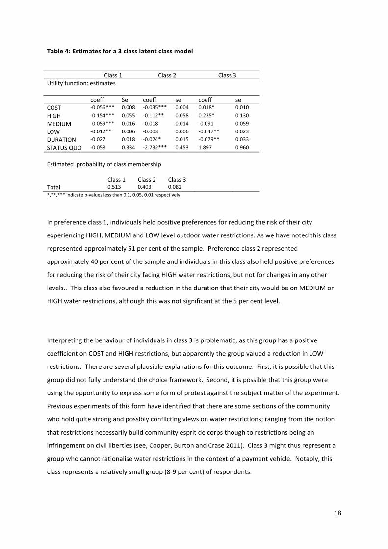
Table 4 reports the estimated results for the preferred latent class model, a three preference class 

model. The first part of the table (utility function: estimates) reports the parameters and significance 

of attributes in each of the three preference classes compared to the base levels. The second part of 

the Table 4 (Estimated probability of class membership) reports the posterior means of the 

probability of class membership across the sample. In this case, about 51 per cent of the modelled 

sample makes up class 1, 40 per cent form call 2 and around 8 per cent form class 3.  

 

   

                                                            6 This may appear high.  However, given the context of the experiment (i.e. a region with relatively high reliability of supply and limited exposure to drought) we consider this plausible. 

18  

Table 4: Estimates for a 3 class latent class model  

  Class 1  Class 2 Class 3

Utility function: estimates 

  coeff  Se  coeff  se coeff se

COST  ‐0.056***  0.008  ‐0.035***  0.004  0.018*  0.010 

HIGH  ‐0.154***  0.055  ‐0.112**  0.058  0.235*  0.130 

MEDIUM  ‐0.059***  0.016  ‐0.018  0.014  ‐0.091  0.059 

LOW  ‐0.012**  0.006  ‐0.003  0.006  ‐0.047**  0.023 

DURATION  ‐0.027  0.018  ‐0.024*  0.015  ‐0.079**  0.033 

STATUS QUO  ‐0.058  0.334  ‐2.732***  0.453  1.897  0.960 

 Estimated  probability of class membership  

   

    Class 1  Class 2  Class 3  

Total  0.513  0.403  0.082     

*,**,*** indicate p‐values less than 0.1, 0.05, 0.01 respectively 

 

In preference class 1, individuals held positive preferences for reducing the risk of their city 

experiencing HIGH, MEDIUM and LOW level outdoor water restrictions. As we have noted this class 

represented approximately 51 per cent of the sample.  Preference class 2 represented 

approximately 40 per cent of the sample and individuals in this class also held positive preferences 

for reducing the risk of their city facing HIGH water restrictions, but not for changes in any other 

levels..  This class also favoured a reduction in the duration that their city would be on MEDIUM or 

HIGH water restrictions, although this was not significant at the 5 per cent level.  

 

Interpreting the behaviour of individuals in class 3 is problematic, as this group has a positive 

coefficient on COST and HIGH restrictions, but apparently the group valued a reduction in LOW 

restrictions.  There are several plausible explanations for this outcome.  First, it is possible that this 

group did not fully understand the choice framework.  Second, it is possible that this group were 

using the opportunity to express some form of protest against the subject matter of the experiment.  

Previous experiments of this form have identified that there are some sections of the community 

who hold quite strong and possibly conflicting views on water restrictions; ranging from the notion 

that restrictions necessarily build community esprit de corps though to restrictions being an 

infringement on civil liberties (see, Cooper, Burton and Crase 2011).  Class 3 might thus represent a 

group who cannot rationalise water restrictions in the context of a payment vehicle.  Notably, this 

class represents a relatively small group (8‐9 per cent) of respondents.   

 

19  

Class membership was estimated using a second stage fractional multi‐nomial logit (MNL) model, 

based on the allocation of individuals to the most likely class, based on the results in Table 4. This 

model preserves the constraint that all class probabilities have to be non‐negative, and sum to unity 

for any individual. This ostensibly allows us to identify if there are significant relationships between 

class membership and other parameters.  Table 5 reports the associated marginal effects (which are 

more informative than the parameters) that can be derived from the fractional MNL model of 

preference class membership. 

 

Table 5 Latent class membership    Class 1  Class 2 Class 3

Latent class membership: marginal effects  

  coeff  Se  coeff  se coeff se

WWR  ‐0.054  0.042  0.024  0.040  0.030**  0.014 

WRESTR  ‐0.007  0.043  ‐0.046  0.041  0.053***  0.015 

GENDER  0.147**  0.064  ‐0.102  0.062  ‐0.045  0.024 

POOL  ‐0.153**  0.072  0.170**  0.069  0.017  0.031 

LONG  0.086**  0.041  ‐0.086**  0.040  0.001  0.017 

SUPPLY1  ‐0.058  0.133  0.109  0.137  ‐0.050**  0.023 

SUPPLY2  0.034  0.160  0.033  0.159  ‐0.067***  0.015 

SUPPLY3  ‐0.030  0.138  0.127  0.141  ‐0.098***  0.032 

SUPPLY6  0.083  0.155  0.188  0.148  ‐0.271  0.178 

**,*** indicate p‐values less than 0.05, 0.01 respectively By definition, the sum of coefficients across the 3 classes is constrained to sum to zero 

  

A set of attitudinal and socio‐demographic variables significantly explain preference class 

membership. More specifically, these variables have a significant marginal effect on the probability 

of class membership.  

 

In the case of class 1, the gender (GENDER) of the respondent, whether the respondent has an 

outdoor pool or spa (POOL) and the duration of residence in the study location (LONG) significantly 

explain membership of this class. More specifically, female respondents, those with no outdoor pool 

or spa, and those that have lived in the study location for longer have a higher probability of class 

membership for Class 1, relative to others in the sample.  

 

20  

Alternatively, in preference class 2, the probability of class membership is increased if a respondent 

has a household with an outdoor pool or spa (POOL) and has lived in the study location for a shorter 

duration.  

 

Stronger preferences for water wises rules (WWR) tend to increase class membership for class 3. In 

addition, those with negative attitudes towards water restrictions (e.g. too costly, unfair, pointless) 

are also more likely to be in class 3. Moreover, respondents who do not have access to recycled 

water, groundwater (e.g. bore, spring) and rainwater tanks are also more likely to be a member of 

this class.  The mixed nature of these variables again supports the view that this class is best 

regarded as a mix of protest respondents. 

 

Table 6 presents estimates of marginal effects for the different attributes. Respondents’ preferences 

are described in terms of their WTP for changes in the levels of the attribute compared to defined 

base levels. For example, if the probability of a water restriction is reduced, the probability of “no 

restriction” is increased equivalently). It would also be possible to estimate the value for shifting to a 

lower level of risk, rather than complete removal. 

 

The values reported in Table 6 are the median values of distributions derived from 10,000 

simulations of parameters drawn from the estimated parameter and variance covariance matrixes 

(Krinsky and Robb 1986), and then the WTP generated as the conventional ratio. 

 

Table 6  Willingness to Pay ($/house/year) for a 1 per cent reduction in the probability of a water 

restriction of that level being imposed (and a 1 per cent increase in probability of no restriction).  

  Class 1  95% Confidence Interval 

Class 2 95% Confidence Interval 

High  +2.72*** 1.039‐4.406 +3.16** 0.581‐5.742 Medium  +1.05*** 0.589‐1.512 +0.51 ‐0.178‐1.214 Low  +0.22**  0.037‐0.395 +0.07 ‐0.210‐0.357 *,**,*** indicate p‐values less than 0.1, 0.05, 0.01 respectively 

 

As we have noted respondents belonging to preference class 1 have positive preferences for a 

reduction in the probability of experiencing HIGH, MEDIUM and LOW water restrictions. Willingness 

21  

to pay is positive and significant at the 95 per cent level of confidence (or greater) for this class. For 

example, respondents in this class, on average, are willing to pay $2.72 for a 1 per cent reduction in 

the probability of experiencing HIGH water restrictions during drought.  Positive preferences for a 

reduction in the probability of HIGH water restrictions are apparent for respondents in class 2. At the 

95 per cent level of confidence this group is willing to pay $3.16 for a 1 per cent reduction in the 

probability of experiencing this level of restriction in drought, on average.  In the case of class 2 the 

lower bound willingness to pay is $0.58 and the upper bound is $5.74 for removing a 1 per cent 

chance of experiencing HIGH water restrictions.   

 

The estimates suggest that participants in class 1 are willing to pay, on average, approximately 

$13.60 (i.e. $2.72*5) per annum for 4 years to remove the 5 per cent probability of experiencing 

HIGH water restrictions, as described in the ‘status quo’, such that there are no water restrictions of 

this form.  More specifically, participants in class 1 are willing to pay approximately $13.60 per 

annum for 4 years to move from a scenario where the likelihood of facing water restrictions is 5 per 

cent for HIGH; 21 per cent for MEDIUM; 47 per cent for LOW; and 27 per cent for NONE to a 

scenario where the chance of facing HIGH water restrictions is 0 per cent; but remains at 21 per cent 

for MEDIUM; 47 per cent for LOW and is thus 32 per cent for NONE (the risk of facing HIGH 

restrictions has been shifted to the NO restriction category).  

 

Alternatively, class 2 individuals are on average willing to pay approximately $15.80 ($3.16*5) per 

annum for 4 years to remove the 5 per cent probability of facing HIGH water restrictions, and move 

that probability to no water restrictions. 

 

The estimates in Table 6 can also be used to determine the willingness to pay to remove the chance 

of experiencing all levels of water restrictions. In addition, it is possible to estimate the trade‐offs 

that respondents within this class will make between the risks of experiencing different levels of 

water restrictions.  

 

The willingness to pay for a reduction in the duration of time the city faces MEDIUM or HIGH water 

restrictions is not significant at the 95 per cent level of confidence.  

22  

 

Clearly, these findings suggest that ‘increased water availability’ options are valued by particular 

segments of customers.  Importantly, the empirical estimates can be adjusted to inform water 

augmentation decisions in a way that is conducive to adaptive management and planning when 

there is uncertainty.  

 

6. Discussion and concluding remarks 

This study sought to investigate households’ WTP to avoid behavioural restrictions placed on water 

use during drought.  The particular focus was to generate WTP estimates that could inform more 

adaptive decision‐making. 

 

Recall that respondents were asked to make choices as if they were entering a drought restriction 

period.  Our rational for taking this approach was that the resulting estimates would then be 

grounded in a scenario that could be adjusted by the planner as additional information came to 

hand without the need for additional choice experiments to enumerate household welfare.  For 

example, with these data the planner can estimate the community benefit of avoiding different 

severities of water restrictions and then compare this against the cost of alternative portfolios of 

supply with differing reliabilities. 

 

The limit of this approach is that the water planner then needs to match hydrological information to 

the drought trigger scenarios.  Because this type of planning can be costly and because some larger 

projects can be staged, these Choice Modelling data are most useful for fine‐tuning the deployment 

of the more costly components of the water supply portfolios.  For instance, the WTP estimates 

could feasibly be integrated with the impacts of large‐scale projects on hydrology/water restrictions 

while varying the water in storage.  This might then allow the planner to optimise the deployment of 

various stages of a project against the water in storage. 

The study found that there was a positive WTP to avoid drought restrictions and that this varied with 

the nature of the behavioural constraints.  More severe restrictions attracted a higher WTP than less 

severe restrictions, on average.  

23  

 

The choice experiment revealed that the preferences for paying to alleviate water restrictions were 

heterogeneous.  A sizeable portion of the sample appeared to protest against the notion of paying to 

reduce the risk of water restrictions.  Nonetheless, our estimates of the total welfare gains from 

eliminating water restrictions are also significant. 

 

The welfare estimates generated by this experiment raise questions about the extent to which these 

data support the introduction of more severe or more frequent water restrictions.  It is important to 

note that the data collected for this experiment were framed as ‘willingness to pay’ which aligns 

with consumers making a payment to secure an improvement in welfare (as symbolised by a 

reduction in water restrictions).  In that regard the data provide a basis for comparing investments 

that would reduce the need for water restrictions.  Thus, modest willingness to pay for reducing 

water restrictions should not be used to advocate for more stringent or more frequent water 

restrictions.   Rather, modest willingness to pay simply limits the case for measures that alleviate the 

need for restrictions.   

 

The assembled data have primarily been used to answer questions about the cost effectiveness of 

water portfolios.  Nonetheless, more could be made of this information, including more detailed 

analysis of the motivations that shape willingness to pay and the nature of protest in this context.  

Another important extension would be to test the assumptions that allow for the wider use of these 

data.  This could include investigation of any links between willingness to pay and willingness to 

accept in this setting.   

 

References 

Australian Bureau of Statistice (ABS) (2013), Population by age and sex, regions of Australia, 2012, 

URL: http://www.abs.gov.au/Ausstats/abs@.nsf/mf/3235.0, (Accessed on 30 August 2013). 

Ben‐David, R. (2013), Paying for the Victorian desalination plant: A case study in regulatory ambiguity. Water 2013 Conference: Affordability, Liveability and Efficiency. Sydney: IIR. 

Brennan, D., S. Tapsuwan, and G. Ingram (2007), The welfare costs of urban outdoor water 

restrictions, The Australian Journal of Agricultural and Resource Economics, 51(3), 243‐261. 

24  

Clarke, H. (2014), “Real Option and Insurance Approaches to Evaluating Infrastructure Projects 

Under Risk and Uncertainty: A Checklist of Issues”, Australian Economic Review, 47, 1, 2014, 147‐

156. 

Cooper, B., Burton, M. and Crase, L. (2014), Avoiding Water Restrictions in Australia: Using A Finite 

Mixture, Scaled Ordered Probit Model to Investigate the Impact of Changes to the Climatic Setting, 

World Congress of Environment and Resource Economists, Istanbul, Turkey, 28 June‐2 July. 

Cooper, B., Burton, M. and Crase, L. (2011), Urban Water Restrictions: Attitudes and Avoidance, 

Water Resources Research. 47, W12527, doi: 10.1029/2010WR010226, 2011. 

Cooper, B., Rose, J. and Crase, L. (2012), Does Anybody Like Water Restrictions? Some Observations 

in Australian Urban Communities, Australian Journal of Agricultural and Resource Economics. 56 (1), 

pp.61‐81. 

Edwards, G. (2008), Urban water management. In Water policy in Australia: the impact of change 

and uncertainty, ed. L. Crase, L. Washington: RFF Press. 

Fleming, C. and Cook, A. (2007), Web surveys, sample bias and the travel cost method. Proceedings 

of the 51st Annual Conference of the Australian Agricultural and Resource Economics Society, 

Queenstown February 13‐16, 2007, New Zealand.Oehlert, G. W. 1992. A note on the delta method. 

American Statistician 46: 27–29. 

Hensher, D., Rose, J. and Greene, W.  (2005), Applied choice analysis: a prime. Cambridge, United 

Kingdom. 

Hensher, D., N. Shore, and K. Train (2006), Water supply security and willingness to pay to avoid 

drought restrictions. Economics Record. 256(82), 56‐66. 

Hole AR. (2008), Modelling heterogeneity in patients’ preferences for the attributes of a general 

practitioner appointment. Journal of Health Economics 27: 1078–1094. 

McFadden D, Train K. (2000), Mixed MNL models for discrete response. Journal of Applied 

Econometrics 15: 447‐470. 

Nylund K, Asparouhov T, Muthen B. (2007), Deciding on the number of classes in latent class analysis 

and growth mixture modelling: a Monte Carlo simulation study. Structural Equation Modelling 14: 

535‐569. 

Productivity Commission. (2011), Australia’s Urban Water Sector, P.C, Melbourne (available at: 

http://www.pc.gov.au/projects/inquiry/urban‐water/report)  

Scarpa, R. and Rose, J. (2008), Design efficiency for non‐market valuation with choice modelling: how 

to measure it, what to report and why, The Australian Journal of Agricultural and Resource 

Economics, 52(3), 253‐282. 

Swait, Joffre (1994), A Structural Equation Model of Latent Segmentation and Product Choice for 

Cross‐Sectional Revealed Preference Choice Data, Journal of Retailing and Consumer Services, 1 

(April), 77–89. 

25  

Train K. (2009), Discrete choice models with simulation. 2nd ed. Cambridge University Press: New 

York, NY.  

Vermunt, J. K. (2010), Latent Class Modeling with Covariates: Two Improved Three‐Step Approaches, 

Political Analysis, 18: 450‐469.