modeling the fishing behavior for the galapagos lobster...

1 | P a g e

Modeling the Fishing Behavior for the Galapagos Lobster Fishery

S. Bucaram1, J. Sanchirico2, and J. Wilen3 1PhD. Candidate, Agricultural and Resource Economics Department, University of California at Davis.

2Professor, Department of Environmental Science and Policy, University of California at Davis. 3Professor, Agricultural and Resource Economics Department, University of California at Davis.

Selected Paper prepared for presentation at the Agricultural & Applied Economics Association’s 2012 AAEA Annual Meeting, Seattle, Washington, August 12-14, 2012

Copyright 2012 by S. Bucaram, J. Sanchirico and J. Wilen. All rights reserved. Readers may make verbatim copies of this document for non-commercial purposes by any means, provided

that this copyright notice appears on all such copies.

2 | P a g e

1. INTRODUCTION

The overexploitation of the two more profitable marine species in the GMR (i.e. the red spiny

lobster and the sea cucumber) confirms the prejudicial effects that command and control policies

have had over the biological health of the marine resources in the Galapagos Islands during the last

14 years. In spite of that, the consensus of fisheries scientists that have worked in the Galapagos is

that, it is not the quality of policies applied up today there, but the moral character and in some cases

the cultural traits of the Galapagos fishermen the root of the fisheries problem in the GMR. In other

words, they have concluded that the main cause of the fisheries problems in the Galapagos is the

“bad behavior” of fishermen. Hence, there are those who have argued that fishermen suffer of

shortsightedness which induces them to prefer short-term economic growth strategies that require

the exhaustive exploitation of marine resources in the present (González et. al. 2008, Ospina 2006).

There are others who asserted that the problem is the origin of fishermen. That is, that given that

most of Galapagos fishermen migrated from mainland; they possess a “Frontier Mentality” and not

an “Island Mentality” (Ospina 2006). In other words, it is asserted that Galapagos fishermen do not

have a culture of ecological awareness about what implies living on the Islands, therefore they are

unable to live sustainably there and they even have a depredatory view of the natural resources

(Hearn 2008, Hardner 2004, Ospina 2006). And finally there are those who claim that greed is the

root of the fisheries problem in the Galapagos Islands and therefore it doesn’t have any solution

(Sea Sheppard 2004, Toral 2008). Based on these arguments, fisheries scientists have arrived to a

conclusion, that the only fisheries policies that make sense for the GMR are those that restrain the

bad behavior of fishermen. In other words restrictive policies imposed by the authorities for the

greater good of the society and the environment.

3 | P a g e

This has been the rationale in which the decision of imposing conventional regulatory

policies is grounded; all of them command and control policies whose aim is to control fishing

mortality through policing continuously the bad behavior of fishermen in Galapagos. According to

those fishermen scientists this type of policies would assure the proper protection of the marine

resources. But if the results are not like the expected ones (as actually has happened in the

Galapagos Islands) the failure is attributed to a political process that does not listen to scientists (a

claim that has also been frequently enunciated during these 14 years in the Galapagos).

However the rational process used by those fisheries scientists to propose their policy

recommendations is flawed. This is because they have failed to characterize this “bad behavior” of

fishermen first; and even worse they have not explained the reasons that motivate that behavior. As

far as we know, there are not studies that try to describe and to explain the fishing behavior in the

Galapagos Islands or that attempt to determine the factors that influence that behavior. Hence in

this paper we expect to fill that gap in the literature through modeling and analyzing the fishing

behavior of Galapagos fishing units of production (FUP) for the Red Spiny Lobster Fishery. We

will determine what factors are determinant for the participation decision of FUPs for the lobster

fishery as well as what factors are relevant for their frequency of participation after they have

decided to participate.

Finally an important observation before starting is that the analyses for this paper will be

based on the red spiny lobster fishery only. Then, when we refer to a fishing season in this paper,

keep in mind that we are talking about the red spiny lobster season which lasts four months from

September to December of any year.

4 | P a g e

2. CLASIFICATION OF FISHERMEN AND VESSELS IN THE GALAPAGOS

FISHERIES.

The Galapagos National Park (GNP), the regulatory authority of the GMR, has classified fishermen

into two categories: armadores and pescadores. Armadores are those fishermen who have at least

one ship (i.e. panga, fibra or bote) and Pescadores are fishermen who do not possess any ship at all.

According to the GNP’s official record, 61.3% of the registered fishermen are classified as

“pescadores”, while the remaining 38.7% are classified as “armadores”1. Thus vessels, which are

considered as capital in this production system, are owned by a minority of fishermen.

There is another peculiarity in the relationship between armadores and vessels; this is that

the ratio between registered vessels and registered armadores was equal to 0.83 in 2008. This

indicates that some armadores owns more than one vessel. Even more, if we analyze a little more

about this issue we find that during the period 2001-2008 the proportion of armadores who own

more than one boat increased from a minimum of 9.72% in 2003 to a maximum of 13.98% in 2008

(Table 1). There was also an increment of more than 100% in the number of people who own more

than two boats in 2008. This is an interesting trend, especially because happened in a moment in

time when the health of the two most profitable fisheries is highly deteriorated. At the end this

dynamic has produced that those boats that are owned by armadores who have multiple boats

increase from 21.5% to 28.2% of the total number of registered vessels. This trend of accumulating

boats in very few owners is a trend that hasn’t stopped in the last years but it has accentuated.

According to the 2011 Lobster Fishery Report (GNP 2011) approximately 18% of armadores owned

more than one boat up today. Hence, as we previously said, this is an interesting trend because

1 Pescadores are considered as labor for this production system.

5 | P a g e

occurs in a moment in which the profitability of the fishery activity has fallen, especially because of

the collapse of the sea cucumber fishery and the contraction of the lobster fishery. Yet more, we

observe that this trend started to accentuate after 2006, the year in which many considered that the

sea cucumber fishery had collapsed.

Table 1. Classification of armadores based on the number of vessels that they own Number of vessels 2001 2002 2003 2004 2005 2006 2007 2008

1 350 358 362 362 350 350 332 320 2 38 38 37 37 40 40 52 46 3 4 4 2 2 4 4 2 6 4 0 0 1 1 1 1 1 4

Total Number of Armadores 392 400 401 401 394 394 386 372

The dynamic of the ownership status of armadores of fishing vessels in the Galapagos

Islands is very important, however we should determine if that dynamic has had an impact on the

fishing behavior. For this purpose we will proceed to analyze if there is any difference in the

participation and frequency of participation between those vessels that are owned by armadores who

own only a boat (AWOOB) and those vessels that are owned by armadores who own multiple boats

(AWOMB). For this purpose, we use a kernel estimation procedure to determine the density

function of the level of participation (after they decide to participate) for those vessels that are

owned by AWOOB, labeled in the graph as one boat, and those vessels that are owned by

AWOMB, labeled in the graph as multiple boats. Thus we observe in Figure 1, that the curve labeled

as multiple boats has more observations concentrated in the left side of the distribution (i.e. region of

low participation) than the curve labeled as one boat. Even more when we conducted a Kolmogorov-

Smirnov test to both distributions we found a D=0.1281 with a Corrected-P-value of 0.000 then we

reject the null hypothesis of equality of distributions for both curve. On the other hand, if we apply

6 | P a g e

the same Kolmogorov-Smirnov test but using instead the variable that represents the decision of

participation in a season for vessels owned by AWOMB or AWOOB, we found a D=0.0442 and a

Corrected-P-Value equal to 0.292. Then we cannot reject the null hypothesis of equality of

distributions for the decision of participations for these two groups. Therefore it can be concluded

that even though the ownership status of the armador who owns an vessel apparently doesn’t have a

differential impact on the decision of participation, there is evidence that this ownership status it

does have an impact on the intensity (or frequency) of participation; in a way that, those boats that

are owned by AWOMB participate less frequently than those boats owned by AWOOB.

Figure 1. Kernel Density Estimation of Intensity of Participation of Vessels

This result is consistent with the observation that armadores not always participate in the

fishing activity but they prefer to provide their ships to pescadores, so that they can use it to fish and

after that to share their profits with those armadores (Castrejon 2009). Then the previous result

05

10D

ensi

ty

0 .1 .2 .3 .4 .5Frequency of Participation

multiple boats one boat

kernel = epanechnikov, bandwidth = 0.0144

Kernel density estimate

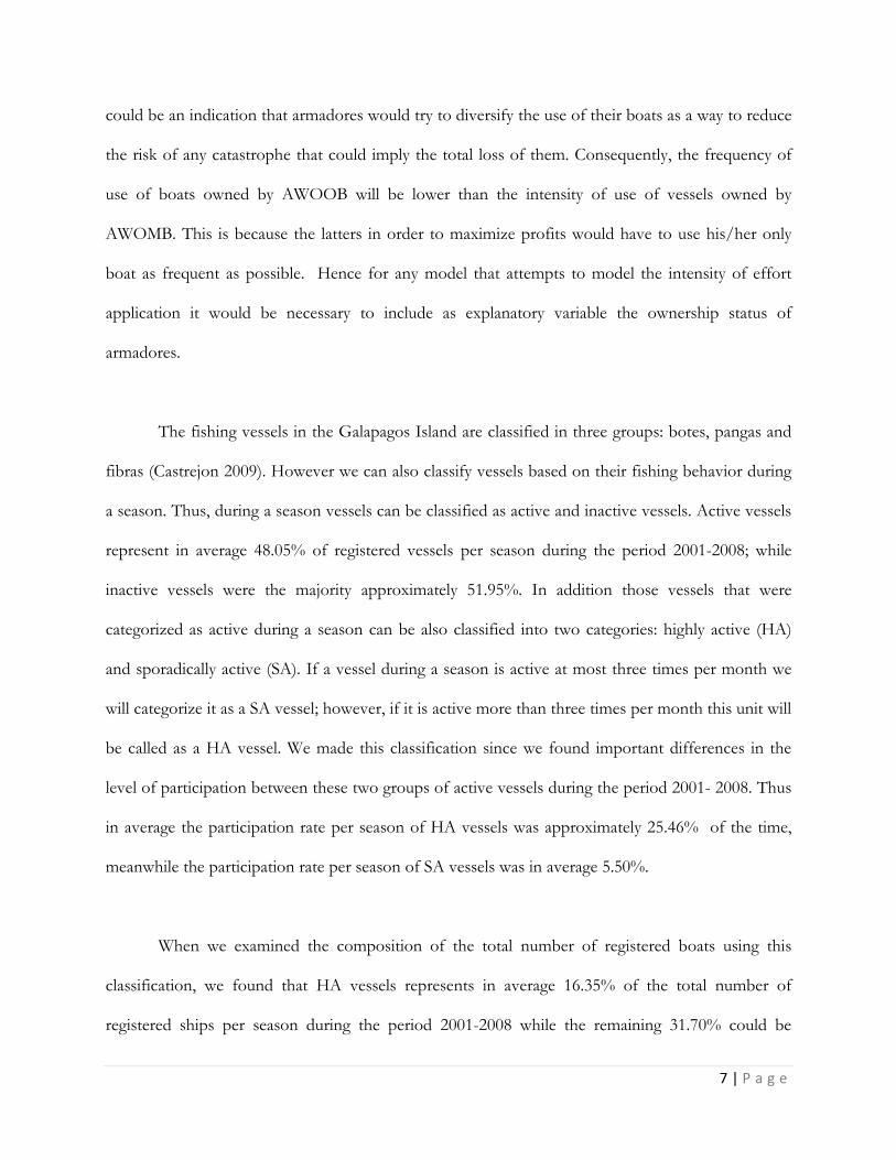
7 | P a g e

could be an indication that armadores would try to diversify the use of their boats as a way to reduce

the risk of any catastrophe that could imply the total loss of them. Consequently, the frequency of

use of boats owned by AWOOB will be lower than the intensity of use of vessels owned by

AWOMB. This is because the latters in order to maximize profits would have to use his/her only

boat as frequent as possible. Hence for any model that attempts to model the intensity of effort

application it would be necessary to include as explanatory variable the ownership status of

armadores.

The fishing vessels in the Galapagos Island are classified in three groups: botes, pangas and

fibras (Castrejon 2009). However we can also classify vessels based on their fishing behavior during

a season. Thus, during a season vessels can be classified as active and inactive vessels. Active vessels

represent in average 48.05% of registered vessels per season during the period 2001-2008; while

inactive vessels were the majority approximately 51.95%. In addition those vessels that were

categorized as active during a season can be also classified into two categories: highly active (HA)

and sporadically active (SA). If a vessel during a season is active at most three times per month we

will categorize it as a SA vessel; however, if it is active more than three times per month this unit will

be called as a HA vessel. We made this classification since we found important differences in the

level of participation between these two groups of active vessels during the period 2001- 2008. Thus

in average the participation rate per season of HA vessels was approximately 25.46% of the time,

meanwhile the participation rate per season of SA vessels was in average 5.50%.

When we examined the composition of the total number of registered boats using this

classification, we found that HA vessels represents in average 16.35% of the total number of

registered ships per season during the period 2001-2008 while the remaining 31.70% could be

8 | P a g e

classified as SA vessels during the same period. That means that the frequency of participation of

approximately 2/3 of the vessels that were active was low (i.e. in average less than 2 days per

month). One of the possible explanations for this phenomenon is that the decision of participation

and the decision of how many days a vessel would be active during a season after deciding to

participate could be highly influenced by the cost of opportunity of alternative activities especially

those related to the tourism sector. Then for modeling the participation decision specially, it is

necessary to include a variable that represents the cost of opportunity derived from available labor

alternatives in the archipelago, like the number of tourists that arrive to the islands per year or the

annual growth rate of tourism.

Finally, it is important to note that there are three ports in the Galapagos Islands, they are:

Puerto Baquerizo Moreno (located in San Cristobal Island), Puerto Villamil (located in Isabela

Island) and Puerto Ayora (located in Santa Cruz Island). The socio-economic conditions in each of

these three ports in the archipelago are completely different therefore the alternative job alternatives

and their derived cost of opportunity for the fishery activity are expected to be different for each

island. For instance Puerto Ayora (PA) is the most economically developed of the three ports and it

is highly active in tourism activities. Puerto Baquerizo Moreno (PBM) has been growing rapidly in

recent years as the tourism sector has been developing with a clear objective of being a direct

competition to PA. Finally, Puerto Villamil (PV) is the less developed of the ports with a tourism

sector very incipient. The perspectives of economic growth of PV are limited due to the reluctance

of its population. Hence we considered important to consider the vessels’ port of origin as a

determinant factor on the observed fishing behavior of them. This is because we assumed that

fishing behavior is influenced by the socio-economic environment and the economic prospects (i.e.

9 | P a g e

cost of opportunity) available to fishermen in their port of origin, since as we indicated, they are

dissimilar in each port.

2.2. CLASSIFICATION OF PANGAS AND FIBRAS BASED ON THEIR FREQUENCY

OF PARTICIPATION

Before proceeding further it is important to highlight two important simplifications that we will

apply along this paper. First, since armadores not always participate in the fishing activity but they

borrow/lease their vessels so that others can use them; we will focus our analysis on each vessel

treating them as an independent FUP; with that we assumed that the fishing crew would try to

maximize the profit derived from each trip. Thus our modeling unit from now on will be individual

vessels. And second, we would focus our analyses to the behavior of two types of vessels only; they

are: pangas and fibras. We will make the latter simplification because botes are mostly used as a

mean of transportation. Henceforth, when pescadores (and armadores) decide to take their fishing

activities to farther locations (such as Darwin and Wolf islands) they hire a bote to transport fibras

and pangas to that specific location. At the end, the catch that is registered is the individual catch for

each fibra and panga that were transported in a bote. The owner of a bote is paid either with money

or with product. Then to avoid problems of double counting we will focus in fibras and pangas only,

which are the more numerous type of vessel in the archipelago anyway (i.e. 85% of the total number

of registered vessels and 95% of the active vessels). Thus from now on when we refer in this paper

to a FUP, we will be talking about pangas and fibras.

In this section we will analyze the composition of FUPs based on their level of participation

(i.e. Inactive, Sporadically Active and Highly Active) as well as the average frequency of participation

for each of these categories. For this purpose we conduct this analysis per island and during the

10 | P a g e

period 2001-2008. In Table 2 we can observe that the composition of FUPs given their level of

activity differs for each port. Thus we observed that San Cristobal is the island with the highest

proportion of inactive FUPs and is also the island with the lowest proportion of FUPs classified as

HA in average per season. On the other hand Santa Cruz is the island with the highest proportion of

FUPs considered HA and also it has the lowest proportion of inactive FUPs. On the other hand we

found (Table 3) that there are small differences in the average level of participation per season for

each type of active FUPs (i.e. highly active and sporadically active) in each island. However, these

differences are similar with those found in the average composition of FUPs showed in Table 2.

Hence, San Cristobal is the island that showed the lowest level of participation for both type of

active FUPs and Santa Cruz is the island that showed the highest for both type too. This indicates

the importance of including location regressors when modeling the choices for participation and

intensity of participation in the Galapagos Island for FUPs.

Table 2. Percentage of FUPs classified based on their participation by island

Classification Isabela San Cristobal

Santa Cruz

Inactive 53.50% 53.90% 46.64% Sporadically Active 26.83% 34.73% 31.31% Highly Active 19.67% 11.37% 22.05%

Table 3. Frequency of participation (days active divided by total number of days per season) of FUPs by island

Type of Vessel Isabela San Cristobal Santa Cruz

Mean Std. Dev. Mean Std. Dev. Mean

Std. Dev.

Sporadically Active 6.09% 4.15% 5.01% 3.83% 6.11% 4.28% Highly Active 24.98% 17.80% 23.35% 7.52% 26.86% 10.54%

11 | P a g e

Figure 2. Kernel Density Estimation for the Frequency of Participation of FUPs in San Cristobal

Figure 3. Kernel Density Estimation for the Frequency of Participation of FUPs in Santa Cruz

05

1015

Den

sity

0 .1 .2 .3 .4 .5Frequency of Participation

Sporadically Active Highly Active


Kernel density estimate0

24

68

10D

ensi

ty

0 .2 .4 .6Frequency of Participation




12 | P a g e

Figure 4. Kernel Density Estimation for the Frequency of Participation of FUPs in Isabela

Finally, when we analyze the frequency of participation between the two different classes of

active FUPs (i.e. SA and HA) using a set of kernel densities (Figure 2 to 4) we found out a striking

difference between the distribution functions of these two categories in each island, which confirms

the rationale of making this classification among active FUPs.

3. ECONOMETRIC MODEL FOR PARTICIPATION AND INTENSITY OF

PARTICIPATION FOR THE LOBSTER FISHERY

In the last section it was shown that there is a high level of non-participation in the lobster fishery

but also that among those FUPs that participate there is a high percentage with a low frequency of

participation. For this reason we considered that it is important to examine the factors that influence

these fishing behaviors in the Galapagos lobster fishery.

02

46

810

Den

sity

0 .2 .4 .6Frequency of Participation




13 | P a g e

Hence we are interested in estimating two models, the first one for the decision of

participation in a fishing season (yes or no) and the second for the decision about frequency of

participation after a FUP has decided to participate. Specifically the relationship that we will

estimate to explain the frequency of participation is as follows:

ln�𝑓𝑖,𝑗,𝑦 + 1� = 𝛽1𝑙𝑛 �1 + CPUE𝐿𝑜𝑏𝑠𝑡𝑒𝑟,𝑖,𝑦−1� + 𝛽2𝑙𝑛�1 + CPUE𝑆𝑒𝑎 𝐶𝑢𝑐𝑢𝑚𝑏𝑒𝑟,𝑖,𝑦−1� +

𝛽3𝑑𝐼𝑠𝑎𝑏𝑒𝑙𝑎 + 𝛽4𝑑𝑆𝑎𝑛 𝐶𝑟𝑖𝑠𝑡𝑜𝑏𝑎𝑙 + 𝛽5𝑑𝐴𝑊𝑂𝑀𝐵 + 𝜀𝑖,𝑗,𝑦 iff 𝑓𝑖,𝑗,𝑦 > 0 (1)

where f is the frequency of participation measured as the ratio between the number of days that a

FUP was active and the total days of a season (i.e. 122 days); CPUE𝐿𝑜𝑏𝑠𝑡𝑒𝑟,𝑦−1 is the average CPUE

of a FUP on the lobster fishery during the previous season; and CPUE𝑆𝑒𝑎 𝐶𝑢𝑐𝑢𝑚𝑏𝑒𝑟,𝑦−1 is the

average CPUE of a FUP on the sea cucumber fishery during the previous season. We also included

two dummy variables for the port of origin of the FUP (𝑑𝑆𝑎𝑛 𝐶𝑟𝑖𝑠𝑡𝑜𝑏𝑎𝑙 and 𝑑𝐼𝑠𝑎𝑏𝑒𝑙𝑎) and an

additional dummy to gather the effect of the ownership status of the armador related to a FUP

(𝑑𝐴𝑊𝑂𝑀𝐵). FUPs are denoted by the subscript i and armadores by j. Time is indexed by year and will

be represented by the subscript y.

On the other hand the relationship that we will estimate to explain the decision of

participation is the following:

𝑝𝑖,𝑗,𝑦 = Θ�𝛼1𝑙𝑛�1 + CPUE𝐿𝑜𝑏𝑠𝑡𝑒𝑟,𝑖,𝑦−1� + 𝛼2𝑙𝑛�1 + CPUE𝑆𝑒𝑎 𝐶𝑢𝑐𝑢𝑚𝑏𝑒𝑟,𝑖,𝑦−1� +

𝛼3𝑑𝐼𝑠𝑎𝑏𝑒𝑙𝑎 + 𝛼4𝑑𝑆𝑎𝑛 𝐶𝑟𝑖𝑠𝑡𝑜𝑏𝑎𝑙 + 𝛼5𝑑𝐴𝑊𝑂𝑀𝐵 + 𝛼6𝑇𝑜𝑢𝑟𝑖𝑠𝑚𝑦−1� + 𝑢𝑖,𝑗,𝑦 (2)

14 | P a g e

where p is the participation status of a FUP in the lobster fishery in any given season. This variable

takes a value of one if the FUP participates in the lobster season (regardless of the frequency) and

zero otherwise. Most of the explanatory variables were explained for the previous model (equation

1) except for the variable 𝑇𝑜𝑢𝑟𝑖𝑠𝑚𝑦−1 which represents the total number of tourist that entered to

the Galapagos Islands in the 12 months previous to the opening of a lobster season.

It is important to specify that in equation 2 the cumulative distribution function Θ[∙] can be

defined in two ways; that is, as a normal or as a logistic distribution. If we define Θ[∙] using a normal

distribution we would obtain a linear probit model. On the other hand if we use the logistic

distribution to define Θ[∙] we obtain the linear logistic regression. Along this paper we will use both

distributions to estimate equation 2.

It is important to note that in both specifications (equations 1 and 2) we did not include a

variable related to the type of FUP (i.e. panga or fibra). We decided to not include this variable

because it is highly correlated with the location dummies. Thus when we conducted an analysis of

statistical independence between location and type of FUP variables we determined a critical value

of 253.0824 for the Pearson chi2 and a critical value of 257.8795 for the LR chi2 test; then we reject

the null hypothesis of independence between these two variables. We even found a clear

overrepresentation of Pangas in San Cristobal and Fibras in Isabela. Even more, we determined in

some preliminary estimations that when we include a variable that define the type of vessel along

with location dummies in a model specification, the former lost any statistical significance due to the

effect of multicolinearity with the latters. Thus we decide to drop out the variables related to the

type of FUP for the final specifications that we will use in this paper (equations 1 and 2).

15 | P a g e

In addition, for our estimation work we will use initially a Heckman Selection Model, since it

is very likely that there could be a selection bias process that could be affecting the decision of

frequency of participation. This bias could arise from a selection process that could appear during

the decision of participation due to some unobservable characteristics of either armadores or the

fishing crew. For this purpose we will proceed to estimate a Heckman model first and with that we

verified whether the selection variable (either the mills ratio for the two step procedure or the rho

for the MLE version) is statistically significant or not. If that variable is not significant then we

would reject the hypothesis of the existence of selection bias by unobservable factors and

consequently we would proceed to model both the participation decision and the level of intensity

decision separately. The former, through the use of panel data models and the latter through the use

of Logit and Probit models. Thus in this part we will show the results of those estimations but first

we will provide a description of the data available for that purpose.

3.1. DESCRIPTION OF THE DATA

For the estimations of the models on this paper we will use landings data for the lobster fisheries

collected during the period 2001-2008. This data was collected by the CDF and the GNP during two

different periods. Hence, the subsample of observations corresponding to the period 1999-2006 was

collected by the CDF; and the rest of the sample (i.e. 2007-2009) was collected by the GNP. We

will also use the landings data of the sea cucumber fishery during the same period, 2001 – 2008.

Likewise we will utilize information about which boats and fishermen were legally able to

participate in any fishery activity in the Galapagos Islands. We obtained that data from the

Galapagos Fishery Record (GFR) which is managed by the GNP. The year 2001 is the first in which

we have available data of that type since that year was used as baseline for the process of registration

16 | P a g e

in the GFR, which was officially closed by 2002. Before that time, there was not any kind of official

registration of vessels or fishermen, except for the membership records to the fishing cooperatives,

which is confidential information. Thus we will use the information from the GFR along with the

landings data to determine which vessels participated in a specific lobster fishing season and with

that to identify their characteristics (especially to classify if the vessel was a panga or a fibra) as well

as who the owners of any of those vessels were. Finally, we obtained data about the total number of

tourist that has entered to the island per year as well as the rate of growth of tourism. This would

work as a proxy variable for the job opportunities that fishermen have available during any given

season.

Table 4 gives descriptive statistics for the 2,688 observations that comprise the estimation

sample.

Table 4. Descriptive Statistics of Variables Variable Mean Std. Dev. Min Max 1. Participation 0.494 0.500 0 1.0000 2. Frequency of Participation 0.066 0.112 0 0.6417 3. Last Year Average CPUE on the Lobster Fishery (Kg/day) 6.570 10.391 0 76.884 4. Last Year Average CPUE on the Sea Cucumber Fishery (ind./day) 247.369 577.461 0 4,949.667 5. Isabela (Location dummy) 0.303 0.460 0 1 6. San Cristobal (Location dummy) 0.440 0.450 0 1 7. Santa Cruz (Location dummy) 0.257 0.437 0 1 8. AWOMB (dummy indicating the vessel is owned by an AWOMB) 0.220 0.414 0 1 9. Number of tourist for the 12 months previous to a lobster season 107,054 31,342 68,856 161,859

Note: Statistics are based on 2,688 observations.

17 | P a g e

3.2. ECONOMETRIC MODELS I: HECKMAN SELECTION MODELS

In section 2.2, we determined that there is a large level of non-participation in our sample and also

that there is a high percentage of FUPs that after deciding to participate have a low frequency of

participation. This could be an indication of the existence of a self-selection process in the sample,

since it is very likely that the outcome of interest, in this case the level of effort applied to the system

represented by the percentage of time that a boat decide to be active (i.e. intensity of participation),

could be determined by some unobservable characteristics of either armadores or fishing crew that

affect simultaneously the former decision and the individual choice of whether to participate or not

in the fishing activity as well. In order to deal with this potential problem we will apply a Heckman’s

selection model.

The Heckman model is composed by two equations; a selection equation, that in our case will

have the same structure as equation 2 and an outcome equation represented by the process shown in

equation 1. We assume for this system of equations a bivariate normal distribution with zero means

and correlation 𝜌. In other words we assume that:

𝑢𝑖,𝑗,𝑦~𝑁(0,1)

𝜀𝑖,𝑗,𝑦~𝑁(0,𝜎2)

𝑐𝑜𝑟𝑟�𝑢𝑖,𝑗,𝑦, 𝜀𝑖,𝑗,𝑦� = 𝜌

In addition the relationship of interest or outcome equation is a simple linear model of a

dependent variable 𝑓𝑖,𝑗,𝑦 that is observed if and only if a second unobserved latent variable, in our

case 𝑝𝑖,𝑗,𝑦, exceeds a particular threshold (in this case zero). In other words 𝑃𝑟�𝑝𝑖,𝑗,𝑦 = 1� =

Φ(𝑤𝑖′𝛾) which is similar to a Probit process like the one established for equation 2.

18 | P a g e

There are two ways to estimate this model:

a. HECKMAN’S TWO-STEP PROCEDURE

The assumptions of this estimation procedure are that both 𝑢𝑖,𝑗,𝑦 and 𝜀𝑖,𝑗,𝑦 are independent

of the explanatory variables and that 𝑢𝑖,𝑗,𝑦~𝑁(0,1) (Wooldridge 2002). The two-step procedure is

the most common estimation method for the Heckman selection model and is implemented as

follows:

a) Estimate the selection equation (which is a Probit) by MLE to obtain estimates of γ.

b) For each observation in the selected equation, compute: i) the inverse Mill’s ratio which is

equal to: λi�= ϕ(wiγ�)Φ(wiγ�)

where 𝜙 denotes the standard normal density function and Φ is the

standard cumulative distribution; and ii) 𝛿𝚤� = λi��𝜆𝚤� − 𝑤𝑖𝛾��.

c) Estimate 𝛽 and 𝛽𝜆=𝜌𝜎𝜖 by OLS of 𝑓𝑖,𝑗,𝑦 on the vector x and �̂�.

The estimators from this two-step procedure are consistent and asymptotically normal. This

procedure is often called a Heckit model. In this model the coefficient of the inverse Mill’s ratio will

indicate if there is selection bias. If the coefficient is statistically significant, then we know that there

is selection bias, the opposite is also true assuming that the selection equation is specified correctly.

19 | P a g e

b. MLE ESTIMATION PROCEDURE

The Heckman model can also be estimated by MLE; however, this requires making a

stronger assumption than those required for the two-step procedure. For MLE we need to assume

that both 𝑢𝑖,𝑗,𝑦 and 𝜀𝑖,𝑗,𝑦 are distributed bivariate normal with mean zero. It is also necessary

that 𝑢𝑖,𝑗,𝑦~𝑁(0,1), 𝜀𝑖,𝑗,𝑦~𝑁(0,𝜎2) and 𝑐𝑜𝑟𝑟�𝑢𝑖,𝑗,𝑦, 𝜀𝑖,𝑗,𝑦� = 𝜌. Thus the MLE estimation is not

as general as the two-step procedure. In addition, the MLE procedure is less robust than the two-

step procedure, and sometimes it is difficult to get it to converge (Wooldridge 2002). However the

MLE estimation will be more efficient if 𝑢𝑖,𝑗,𝑦 and 𝜀𝑖,𝑗,𝑦 are indeed jointly normally distributed.

It is important to emphasize also that for both estimation procedures an exclusion restriction

is required so as to generate credible estimates. In other words there must be at least one variable

which appears with a non-zero coefficient in the selection equation (equation 2) but does not appear

in the equation of interest (equation 1). If no such variable is available, it may be difficult to correct

for sampling selectivity. The exclusion restriction in this model will be represented by the inclusion

of the variable 𝑇𝑜𝑢𝑟𝑖𝑠𝑚𝑦−1 in the selection equation and not in the outcome equation. This

variable gathered the effect of the growth of the tourism sector. We assume that this variable is

related to the profitability of this sector and therefore it is assumed to be related with the cost of

opportunity of the fishing activity. Then an increase in the number of tourist will increase the

profitability of this activity and will increase the cost of opportunity of participating in the fishing

activity as well. This consequently would affect the participation choice of FUP negatively. We

assume that this variable will affect the choice about the intensity of participation only through its

effect on the participation choice.

20 | P a g e

In addition we have established some ex-ante expectations about the sign of the regressors

in both equations based on results showed previously and some ad hoc assumptions. These ex-ante

expectations are shown in Table 5.

Table 5. Ex-ante Expectations for Sign of Regressors VARIABLES EQUATION 1 EQUATION 2 EXPLANATION

Last Year Average CPUE on the Lobster Fishery (Kg/day)

Positive Positive The more productive the FUP the more likely that he would participate in the lobster fishery and the higher their intensity of participation Last Year Average CPUE on

the Sea Cucumber Fishery (ind/day)

Positive Positive

AWOMB

Negative

Negative

We expect that the ownership status of the armador of a vessel would have a negative effect on both the participation and the frequency of participation choices. However, from the results obtained in section 2.2 we expect that the variable AWOMB will be statistically significant for the frequency of participation equation only. The latter is congruent with the evidence that we found in section 2.2 which indicates that those boats who are owned by AWOMB participate less frequently than those boats owned by AWOOB.

TOURISM N.A. Negative We assumed a positive effect of the tourism over the cost of opportunity of fisheries; therefore we expect that the sign of the variable tourism for the participation model will be negative and statistically significant. In addition it is important to emphasize here that the effect of this variable on the frequency of participation choice will be through its effect on the participation choice only (for that reason we will omit it from eq. 1).

21 | P a g e

3.2.1. ESTIMATION OF HECKMAN MODELS The estimators that we obtained by either the two-step or the MLE procedure, which are shown in

Table 6, satisfied our ex-ante expectations. Thus we found that the past productivity of a FUP

for either the lobster or the sea cucumber fisheries have a positive effect on both the decision of

participation and the decision about frequency of participation. Even more, the productivity on the

lobster fishery has a larger impact on both decisions than the productivity on the sea cucumber

fishery.

We also observe that if a FUP is owned by an AWOMB both decisions will be affected

negatively. However this effect will be only statistically significant for the participation decision, as

we initially expected based on results shown in section 2.2. In addition the variable that represents

the exclusion restriction (i.e. 𝑇𝑜𝑢𝑟𝑖𝑠𝑚𝑦−1) is statistically significant and negative as we expected. In

other words we found that the growth of tourism affects negatively the decision of participation of a

FUP in the lobster fishery because of an increase in the cost of opportunity of fishing.

Finally when we analyzed the significance of the Mill’s ratio, for the two-step estimation

procedure, and the lambda estimator, for the MLE procedure, we found that we cannot reject the

null hypothesis of the no presence of selection bias. Even more when we examined the value of rho

(from the MLE column) we cannot reject the null hypothesis of independence of both equations

either. This indicates that it is possible to analyze econometrically both equations (the outcome and

selection one) separately. We will proceed to do that in the next sections of this paper.

22 | P a g e

TABLE 6. Estimated regressors for Heckman Model VARIABLES 2-step MLE OUTCOME EQUATION

Last Year Average CPUE on the Lobster Fishery (Kg/day) 0.1799*** 0.1549*** (0.0603) (0.0379)

Last Year Average CPUE on the Sea Cucumber Fishery (ind/day) 0.0547*** 0.0435*** (0.0265) (0.0162)

Isabela (Location dummy) 0.3147**** 0.3407*** (0.0968) (0.0834)

San Cristobal (Location dummy) -0.4709*** -0.4526*** (0.0806) (0.0728)

AWOMB -0.2861*** -0.2809*** (0.0746) (0.0737)

Constant term 1.7658*** 1.9116*** (0.3290) (0.1848)

SELECTION EQUATION

Last Year Average CPUE on the Lobster Fishery (Kg/day) 0.3653*** 0.3653*** (0.0216) (0.0216)

Last Year Average CPUE on the Sea Cucumber Fishery (ind/day) 0.1695*** 0.1695*** (0.0095) (0.0095)

Isabela (Location dummy) -0.4371*** -0.4370*** (0.0742) (0.0742)


AWOMB -0.0376 -0.0372 (0.0657) (0.0657)

Tourism -0.0044*** -0.0044*** (0.0009) (0.0009)

Constant Term -0.0949 -0.0936 (0.1138) (0.1139)

Mill's ratio 0.1836 (0.2820)

Lambda 0.0514 (0.1383)

Rho 0.0551 (0.1484)

Number of observations 2,688 2,688 Censored observations 1,359 1,359 Uncensored observations 1,329 1,329

The dependent variable of the outcome equation is the log of the ratio of participation of a vessel and for the selection equation is a binary variable that takes the value of one if a vessel participated in a season and 0 otherwise. Triple asterisk (***) indicates significance at the 1% level (**) at the 5% level and (*) at the 10% level.

23 | P a g e

3.3. ECONOMETRIC MODELS II: FREQUENCY OF PARTICIPATION MODEL

After checking that both the Mill’s ratio (two-step procedure) and the lambda (MLE procedure) for

the estimated Heckman models from last section were not significant, we concluded that there was

not selection bias on the decision for intensity of participation that came from unobservable

characteristics of armadores or the fishing crew. In other words the variables that were used in the

model were enough to characterize the effect of those unobservable characteristics. However we

also found that the estimator of rho in the MLE procedure was not statistically significant, then the

participation choice and the intensity of participation choice are independent. For this purpose we

will proceed to conduct a separate econometric analysis of both decisions.

In this section we estimated a series of models for the decision about how many days a FUP

will be active (compared to the total days of the season length) conditional on the fact that the FUP

has decided to participate in the lobster fishery season. Our first specification models the data

through an Ordinary Least Squared (OLS) with robust standard errors clustered on the armadores

variable. It is very likely that there is correlation within armadores but not across them, then with a

clustered specification for the standard errors we would correct the downward bias of using regular

or robust standard errors.

Our second specification is a Fixed Effect (FE) model2, which is equivalent to an OLS

regression with a full set of armador-specific fixed effects. With this approach we would try to

measure unobserved heterogeneity related to the owner characteristics that could be affecting the

decision about frequency of participation. While the fixed effect estimator is consistent, it is not as

2 We don’t consider a Tobit specification because this model makes a strong assumption; that is, that the same probability mechanism generates both the observations with zero (no participation) and the positives. We proved that this statement was false in the last section, and then we disregard the use of a Tobit.

24 | P a g e

efficient as a Random Effect (RE) estimator if the unobserved armador-specific effect is

uncorrelated with the observed regressors. The RE model treats the armador-specific effects as

random variables that are distributed independently of the regressors. This model is more efficient

than FE when none of the regressors is correlated with the armador-specific effects; however it is

inconsistent when the opposite is true. Then this assumption of no correlation should be assessed

always using a Hausman test and with that to analyze also if a RE is a more adequate approach than

a FE.

It is necessary to specify that in this case our panel data is unbalanced because of the

attrition of some owners and the appearance of new ones. This is not really a problem as long as

the (strong) exogeneity condition is satisfied, which would assure the consistency of the estimates of

either the FE model or RE model (the latter if and only if the Hausman test is satisfied too).

3.3.1. ESTIMATION RESULTS

In table 7, we report the results of estimating equation 1. It is important to remember that for this

model we use only data for which the frequency of participation is greater than zero, therefore the

number of observations is reduced to 1,329; that it is equal to the number of uncensored

observations in the Heckman model.

In addition we would like to indicate that we conducted a Hausman test comparing FE and

RE estimators, which indicated us that the FE model is appropriate (𝜒52 = 24.7). In other words we

reject the assumption of no correlation between the regressors and the random effects. Hence, the

RE effect is not consistent and it would be incorrect to use those estimators to make any inference

and/or prediction. For that reason we decided to omit the results of that specification in table 7 and

25 | P a g e

show only the estimation results for the OLS and FE specification. Also we conduct a test through

which it cannot be rejected the null hypothesis that the data satisfy the exogeneity condition

(F333,990= 1.06) then the results should be consistent, even though we use an unbalanced panel.

Table 7. Estimated regressors for frequency of participation model (Equation 1) VARIABLES OLS FE Last Year Average CPUE on the Lobster Fishery (Kg/day)

0.144*** 0.044*** (0.026) (0.012)

Last Year Average CPUE on the Sea Cucumber Fishery (ind/day)

0.039*** 0.004 (0.010) (0.029)

Isabela (Location dummy) 0.352*** 0.033 (0.105) (0.245)

San Cristobal (Location dummy) -0.445*** -0.277 (0.091) (0.242)

AWOMB -0.279*** 0.022 (0.081) (0.161)

Constant term 1.974*** 2.128*** (0.093) (0.191)

Number of observations 1,329 1,329 Number of groups 334 334 Significance Test for owner fixed effects [ F(333,990) ] 1.857*** R-squared 0.1327 0.1814

The dependent variable is the log of the ratio of participation of a vessel. Triple asterisk (***) indicates significance at the 1% level (**) at the 5% level and (*) at the 10% level.

We can observe in table 7 that for both specifications the sign of the regressors satisfied our

ex-ante expectations. Nonetheless, there are important differences in the significance of the

estimators for these two specifications; then, we observe that all the regressors are statistically

significant in the OLS specification; however for the FE specification the only regressor that is

statistically significant is the one related to the past productivity of the FUP in the lobster fishery.

Regarding to the appropriateness of these two specifications, we find that a joint F-test of the fixed

effects is highly significant thereby open up the consistency of the OLS model to misspecification.

26 | P a g e

However it is important to emphasize that in both specifications the variable related to the past

productivity on the lobster fishery is statistically significant, even though in the FE model the

magnitude of the estimator is lower. Thus it can be concluded that the most important variable that

predicts the level of effort intensity of a FUP in a lobster season is the level of productivity of that

FUP in the previous season in that same fishery. This indicates that there is a persistence effect for

the amount of effort applied to the lobster fishery for those who have been historically more

productive. This is important because indicates that people are rational since they decide to put their

effort based on their ability and past results.

Finally both specifications show a low degree of explanatory power with an R-squared that

range between 0.1327 and 0.1814. Then, we conclude that we can only get a low level of explanation

when we use models that try to explain the intensity of participation in the lobster fishery using

exclusively explanatory variables that are related to previous season activity as well as characteristics

of the boat and their owner. This could indicate that the decision of how much effort to apply in any

given season could be influenced mainly by the actual conditions observed in the season like the

abundance of the product, price of the product and climate factors and not by historical factors.

.

3.4. ECONOMETRIC MODELS II: INTENSITY OF PARTICIPATION MODEL

In the Heckman model the selection equation was characterized by a Probit through which we

explain the probability that a FUP will participate in any given season. In table 8, we report the

results of estimating the same Probit model but using robust standard errors clustered on the

armador variable and also a second specification using a Logit as cumulative distribution function.

27 | P a g e

The results are consistent with our ex-ante expectations; that is, the estimated coefficients

have the signs and the statistical significance that we expected initially given the results obtained for

our descriptive analysis in section 2 and the Heckman model. In addition both specifications show a

good level of explanatory power, with R2 values that range between 0.235 and 0.306. The magnitude

of this R2 can be considered acceptable for this type of binary dependent variable models. Our

conclusion is that this model explains fairly well the participation behavior in the lobster fishery, and

then it is possible to use it for generating some inferences about the marginal impact of each of the

explanatory variables.

Table 8. Estimated regressors for participation model (Equation 2) VARIABLES Probit Logit Last Year Average CPUE on the Lobster Fishery (Kg/day)

0.3653*** 0.6182*** (0.0248) (0.0427)

Last Year Average CPUE on the Sea Cucumber Fishery (ind/day)

0.1695*** 0.28639*** (0.0097) (0.0166)

Isabela (Location dummy) -0.4371*** -0.7644*** (0.0848) (0.1443)


AWOMB -0.0376 -0.0554 (0.0659) (0.1122)

Tourism -0.0044*** -0.0075*** (0.0009) (0.0015)

Constant term -0.0949 -0.1165 (0.1212) (0.2043)

Number of observations 2,688 2,688 McFadden’s R2 0.239 0.241 McFadden’s Adj R2 0.235 0.237 Cragg & Uhler’s R2 0.282 0.284 Efron’s R2 0.305 0.306

The dependent variable is a binary variable that takes the value of one if a vessel participated in a season and 0 otherwise. Triple asterisk (***) indicates significance at the 1% level (**) at the 5% level and (*) at the 10% level.

28 | P a g e

We calculate a set of marginal effects at the mean for each explanatory variable using as

reference the Logit specification. (Table 9). Thus we observed that an increase of 1 Kg/day on the

average CPUE of lobster in the previous year will increase in 10.71% the probability of participation

in the lobster fishery. In the case of the sea cucumber an increment of the CPUE in one individual

per day will increase the probability of participation in the lobster fishery in 4.96%. Likewise a FUP

from Santa Cruz is 18.78% more likely to participate than a FUP from Isabela and 13.59% more

likely to participate than any FUP from San Cristobal. On the other hand if the owner of a FUP is

an AWOMB the probability of participation falls approximately 1.39% but this effect is not

statistically significant. Finally an increment of approximately 5,263 tourists per year will contract the

participation in the lobster fishery on 1%. Thus, since in average, the number of tourist has

increased in 13,500 people per year, the annual contraction on participation on the lobster fishery

because of the tourism can be estimated in approximately 2.6% annually.

Table 9. Marginal effects at the mean

Variable dy/dx Std. Err. z P-value

Last Year Average CPUE on the Lobster Fishery (Kg/day)) 0.1071 0.0074 14.4900 0.0000

Last Year Average CPUE on the Sea Cucumber Fishery (ind/day) 0.0496 0.0029 17.3000 0.0000

Isabela (Location dummy) -0.1878 0.0341 -5.5000 0.0000 San Cristobal (Location dummy) -0.1359 0.0301 -4.5200 0.0000 AWOMB -0.0139 0.0280 -0.4900 0.6210 Tourism -0.0019 0.0004 -5.0700 0.0000

All these results indicates that the most important factor that affect the participation decision

on the lobster fishery is the last year productivity of the FUP (in lobster and sea cucumber fisheries).

Then a unit of increment in the CPUE of both fisheries (i.e. 1 KG/day for the lobster and 1

individual/day for the sea cucumber) will increase the probability of participation in approximately

29 | P a g e

15%. Therefore, we conclude (like in the case of equation 1) that there is a persistence of

participation of those FUPs that are more productive year by year. Finally it is also important to

highlight the effect of the tourism on the participation on the lobster fishery, as well as the

difference on participation given the location of the FUP. Both variables indicate the presence of a

strong effect of cost of opportunities from alternative activities on the fishing decisions of FUP in

Galapagos.

4. SUMMARY

In this paper, we were able to determine some specific traits of the observed fishing behavior of

vessels in the Galapagos Islands, as well as those factors that are considered as determinants for that

behavior. Thus we found that during any given lobster fishery season vessels can be classified in

three categories: inactive vessels who are the majority, approximately 52% of the total registered

vessels, and active vessels that represent 48% of this group. However we also found important

differences in the level of participation of active vessels, which allow us to divide this group into two

sub-groups: highly active (HA) and sporadically active (SA). We found that 2/3 of active vessels in

any given lobster fishery season can be classified as SA, which have a participation rate of 5.50%;

while the remaining 1/3 of can be classified as HA with a participation rate of 25.46%.

Logit and Probit models revealed that the past productivity of a FUP (defined in this paper

as pangas and fibras only) in the lobster and the sea cucumber fisheries is a good predictor for the

participation choice of any FUP in the lobster fishery. On the other hand, when we analyze the

decision about the intensity of participation we found that only the past productivity of the FUP in

the same lobster fishery is a good predictor for that decision. We also determined that tourism will

30 | P a g e

affect negatively the decision of participation for FUP; this is because this variable represents an

increase in the cost of opportunity of fishing.

The ownership status of the armador will also have an impact on the frequency of

participation of a FUP but not in its decision of participation. In other words we found that if a

FUP is owned by an AWOMB the intensity of participation will be lower than if the same FUP is

owned by an AWOOB. This result is consistent with the observation that armadores not always

participate in the fishing activity but they prefer to provide their vessel to other pescadores, so that

they can use it to fish and after that to share the profits with them. Then it is likely that in order to

reduce the risk of any catastrophe (that could imply the total loss of a vessel) armadores would

diversify the use of their boats if they have more than one.

Finally we found that the goodness of fit of models that try to describe the intensity of

participation using historical data is low. This clearly indicates that the decision about how frequent

to participate in any given season could be influenced not by historical factors but mainly by the

actual conditions observed during the same season. This justifies the use of other econometric

structures that employ this type of current variables like GEV models for further works.

31 | P a g e

REFERENCES

Castrejón, M. 2009. Co-Manejo Pesquero en la Reserva Marina de Galápagos: Tendencias, Retos y Perspectivas de Cambio. Fundación Charles Darwin. Puerto Ayora, Galápagos, Ecuador.

Charles Darwin Foundation and Parque Nacional Galapagos. 1999. La pesca de langostas en

Galápagos en 1998: Un resumen comparativo con la temporada 1997. Informe Preliminar. Puerto Ayora.

Charles Darwin Foundation, Parque Nacional Galapagos, Instituto Nacional de Pesca. 1999. La

pesca de pepino de mar en Galápagos: Periodo abril a mayo 1999. Informe Final. Puerto Ayora, Galápagos.

Edgar, G., S. Banks, J. Fariña, M. Calvopiña and C. Martinez. 2004. Regional biogeography of

shallow reef fish and macro-invertebrate communities in the Galápagos archipelago. Journal of Biogeography 31, 1107-1124.

Epler, B. 1993. An Economic and Social Analysis of Tourism in the Galápagos Islands. Coastal

Resources Center. University of Rhode Island. Narragansett, RI. Epler, B. 2007. Tourism, the Economy, Population Growth, and Conservation in Galápagos.

Charles Darwin Foundation. Puerto Ayora, Santa Cruz Island, Galápagos Islands, Ecuador. FAO (Food and Agricultural Organization of the United Nations). 2005. Review of the State of

World Marine Fishery Resources. FAO Fisheries Technical Paper 475, Rome, Italy. FAO (Food and Agricultural Organization of the United Nations). 1993. Marine fisheries and the

law of the sea: a decade of change. Page 35 in The state of food and agriculture, 1992. FAO Fisheries Circular No. 853FIDI/C583, Rome.

Galapagos National Park (2010). Informa Tecnico de la Pesqueria de Langosta 2009. Galapagos

National Park. Puerto Ayora, Santa Cruz Island, Galápagos Islands, Ecuador. Galapagos National Park (2011). Informa Tecnico de la Pesqueria de Langosta 2010. Galapagos

National Park. Puerto Ayora, Santa Cruz Island, Galápagos Islands, Ecuador. González, J. A., C. Montes, J. Rodríguez, and W. Tapia. 2008. Rethinking the Galapagos Islands as a

complex social-ecological system: implications for conservation and management. Ecology and Society 13: 13.

Hardner, J. and P. Gomez (2004), Incorporación de la Mano de Obra del Sector Pesquero Artesanal

en las Actividades Turísticas de Galápagos, Banco Interamericano de Desarrollo (BID), Quito, Ecuador.

Hearn, A. 2008. The rocky path to sustainable fisheries management and conservation in the

Galápagos Marine Reserve. Ocean & Coastal Management 51, 567–574

32 | P a g e

Murillo, J., Vizcaino, J., Nicolaides, F., Moreno, J., Espinoza, E., Chasiluisa, C., Andrade, R., Born, B., Villalta, M., Yépez, M. & Molina, L. 2002. Informe tecnico final de la pesqueria del pepino de mar (Stichopus fuscus) en las islas Galápagos, 2001 Analisis comparativo con las pesquerias de 1999 y 2000. Fundacion Charles Darwin/ Parque Nacional Galápagos. 29 pp.

Ospina, P. (2006), Galápagos Naturaleza y Sociedad: Actores Sociales y Conflictos Ambientales,

Quito: Corporacion Editora Nacional and Universidad Andina Simón Bolívar. Sea Shepherd (2004). Victory in the Galapagos. Sea Shepherd News. Sea Shepherd Conservation

Society. Itzehoe, Germany. Toral-Granda, V. 2008. Galápagos Islands: a hotspot of sea cucumber fisheries in Central and South

America. En: V. Toral-Granda, A. Lovatelli and M. Vasconcellos (eds). Sea cucumbers. A global review of fisheries and trade. FAO Fisheries and Aquaculture Technical Paper. No. 516. Rome, FAO. pp. 231–253.

Toral-Granda, M., R. Bustamante, J. Murillo, J., E. Espinoza, E., F. Nicolaides, , P. Martínez, I.

Cedeño, B. Ruttenberg, J. Moreno, C. Chasiluisa, S. Torres, M. Yépez, J. Barreno, R. Andrade, L. Figueroa, M. Piu. 2000. La pesca artesanal en Galápagos, 1999-2000. en: Informe Galápagos 1999-2000. p.53-61. Fundación Natura y el Fondo Mundial para la Naturaleza (WWF).

Wilen, J. 2006. Why fisheries management fails: treating symptoms rather than the cause. Bulletin of

Marine Sciences 78, 529-546.

modeling the fishing behavior for the galapagos lobster...

Documents