1

Nonlinearities in Regional Rice Prices in the Philippines: Evidence from a Smooth

Transition Autoregressive (STAR) Approach

Valerien O. Pede1, Harold Glenn A. Valera

1,4, Mohammad J. Alam

2 and Andrew M.

McKenzie3

1Social Sciences Division International Rice Research Institute (IRRI)

2Department of Agribusiness and Marketing, Bangladesh Agricultural University (BAU)

3Agricultural Economics and Agribusiness, university of Arkansas (UofA)

4Department of Economics, University of Waikato

Selected Paper prepared for presentation at the Agricultural & Applied Economics

Association’s 2013 AAEA & CAES Joint Annual Meeting, Washington,

DC, August 4-6, 2013

(Preliminary draft; please do not cite.)

Abstract: This paper investigates nonlinear dynamics in monthly rice prices of 16

regions in the Philippines at three levels: farm gate, wholesale and retail, over the period

of January 1990 to December 2012. We used a series of tests to investigate whether the

regional prices are characterized by linear processes or non-linear smooth transition

autoregressive (STAR)-type dynamics. Results indicate that STAR-type nonlinearity

exists in several regions, and particularly for farm gate prices. The most common process

is a logistic STAR dynamic characterizing an asymmetric price behavior determined by

two regimes and a smooth switching process.

Key words: nonlinearity, rice price, smooth transition

Copyright 2013 by Valerien O. Pede, Harold Glenn A. Valera, Mohammad J. Alam and

Andrew M. McKenzie. All rights reserved. Readers may make verbatim copies of this

document for non-commercial purposes by any means, provided that this copyright notice

appears on all such copies.

2

1. Introduction

Commodity prices are often subject to government actions through the

implementation of domestic and trade measures such as stockpiling and export bans.

Government actions such as these could be the major sources of the nonlinearity in food

price dynamics, especially for rice to which food policy is mostly prioritized in many

countries. This food policy-focused orientation has historically been pervasive in the

Philippine rice sector, where price stabilization program is implemented by National

Food Authority (NFA). The NFA generally offers to buy rice from farmers when prices

are low during peak harvest seasons, and sell the stored grain to consumers through

licensed outlets when prices are high during the dry season (Yao et al., 2005). This is

consistent with government intervention functions, where there is a stronger price

intervention when it is farther from the market determined price. Due to high budgetary

costs associated with NFA actions to influence both the farmgate and retail prices, the

agency may not respond strongly when the market price is close to the set price. Hence,

the market determined price may follow a random walk close to NFA intervention price.

Moreover, the higher and more volatile the price of rice in the global market, the greater

the probability that the NFA will respond strongly as evident in the stockpiling in 2007.

Besides the government intervention in terms of NFA stocks, rice, like many

agricultural crops is also subject to the influence of weather condition and climate

variability. Rice price dynamic is therefore also dependent on climate variability.

Evidence of a relationship between commodity price dynamic and climate variability has

already been stressed in the literature. Rainfall and temperature are among the two main

factors that determine crop productivity. Also, more and more there are claims that

changes in weather patterns – climate change - have an impact on crop productivity and

also on prices. Variability and change in the climatic conditions may be a source of

nonlinearity in price movement (see for instance Ubilava and Holt, 2013 for a recent

example of climatic induced nonlinearity with respect to vegetable oil prices).

In the economics literature, the term “nonlinear price movement” implies that

stabilizing food supply and demand protects producers and consumers against extreme

short-term spikes and low-frequency price volatility (Braun and Tadesse, 2012). Similar

with prices of other staple food, movement in rice prices can be characterized by

3

nonlinearities and there are at least three reasons to believe a priori that such features

might occur. First, the theory of commodity storage recognizes that an inherent

nonlinearity in commodity prices can arise due to the inability of the market to carry

negative inventories (Shively, 1996). Moreover, inter-temporal price transmission can

arise due to storage behavior and induced changes in rice production, which is

unpredictable to begin with because of its dependence on weather conditions. Second,

policy responses such as stockpiling, price controls and trade restrictions used by several

countries during the global price spikes in 2007 and 2008 have been shown to create

tensions and market disruptions, which cause inter-temporal and spatial nonlinearity in

price transmission across countries and regions (Braun and Tadesse, 2012). And third,

transmission of market shocks along the supply chain (vertical price transmission) is

capable of giving rise to nonlinear price adjustments due to the presence of fixed costs

through various stages of the food chain.

The purpose of this paper is to investigate nonlinearities in regional rice prices

dynamics in the Philippines. In particular, the paper examines whether regional rice

prices at farm, wholesale, and retail levels exhibit nonlinearities. This study has important

implications for research attempting to model impacts of NFA price intervention, and the

degrees of market integration and price transmission in Philippine rice markets. Previous

research in these areas has used linear modeling assumptions. However, there are a

number of factors (e.g. government policy intervention, unstable international markets,

and weather) that could generate nonlinear price behavior, and if the true data-generating

process of Philippine rice prices is inherently nonlinear, policy implications drawn from

linear models are questionable.

2. Literature

There is an extensive literature on price dynamics of agricultural commodities which

considers the issue of whether prices exhibit potential nonlinearities. Evidence on

nonlinear dynamics has been considered as support for the strong form of the degree of

adjustment from one price regime to another, which can be useful for policy-making

purposes in recovering information on structural change in prices. Holt and Craig (2006)

examine the potential nonlinear dynamics in the hog–corn cycle in the U.S. by using a

STAR model of monthly prices of hogs relative to corn, and find evidence of nonlinearity

4

and regime-dependent behavior. Following the same econometric approach, Ubilava

(2012) offers a more recent investigation of nonlinearities in the U.S. soybean-to-corn

price ratio. Ubilava (2012) reveals evidence of asymmetries in the co-movement of corn

and soybean prices, and find structural stability in the price ratio dynamics of these crop

pairs over the study period. In the case of single commodity price dynamics analysis,

Reitz and Westerhoff (2007) examine nonlinearities in monthly prices of cotton,

soybeans, lead, sugar, rice and zinc for the period 1973–2003 using a STAR-GARCH

model. Their model suggests that heterogeneous agents and their nonlinear trading impact

may be responsible for pronounced swings in commodity prices. Employing annual data

for 24 US commodities for the period 1900–2003, Balagtas and Holt (2009) find

evidence of nonlinearities in the prices of sixteen commodities using STAR-type models.

The issue of nonlinearities in commodity prices has also been studied in relation

to the price transmission along the food chain. In this vein, considerable attention within

the price transmission literature put particular importance to regime-switching models

which have been employed in many empirical analyses in investigating the presence of

nonlinear price transmission in food markets (Hassouneh et al., 2009). Goodwin and Holt

(1999) examine price interrelationships and transmission among farm, wholesale, and

retail beef markets in the US using a threshold error correction model. Their results

suggest that the transmission of shocks appears to be largely unidirectional with

information flowing up the marketing channel from farm to wholesale to retail markets

but not in the opposite direction. Mainardi (2001) applies the threshold and smooth

transition cointegration models to quarterly prices of three major wheat producing

countries over the period 1973–1999 and finds evidence that non-linear cointegration

models have substantial explanatory power for international wheat prices. Serra et al.

(2008) test the existence of a long-run relationship between ethanol, corn and oil prices

using a smooth transition vector error correction model (STVECM). They find the

existence of an equilibrium relationship between ethanol, corn and oil prices, with non-

linear adjustment of ethanol prices to deviations from its long-run parity. Moreover,

Ubiliva and Holt (2009) estimate the effect of El Niño Southern Oscillation (ENSO) over

time on market dynamics for eight major vegetable oil prices using STVECM, and

present evidence of strong cointegration between the vegetable oil prices, which exhibit

5

nonlinear behavior conditional on the state of nature and the direction of shocks of the

ENSO anomaly. The long-run relationship between vegetable oil prices and conventional

diesel prices in the EU for the period 2005–2007 is also explored by Peri and Baldi

(2010) who apply threshold cointegration approach. Their results suggest a two-regime

threshold cointegration model for rapeseed oil-diesel price relationship.

While a number of studies have provided reviews of the causes and estimation of

asymmetric price transmission (Ward, 1982; Kinnucan and Forker, 1987; Boyd and

Brorsen, 1988; Griffith and Piggot, 1994; Zhang et al., 1995; Bernard and Willet, 1996;

von Cramon-Taubadel, 1998;; Worth, 2000; Parrot et al., 2001; Romain et al., 2002;

Girapunthong et al., 2004; Frey and Manera, 2005; Vavra and Goodwin, 2005), little

research has been done with respect to vertical price transmission in Philippine rice

markets. The existence of asymmetric price transmission across markets in the Philippine

rice industry was examined by Reeder (2000) and Matriz (2008). Reeder (2000) employs

a symmetry model in estimating the changes in rice prices at different market levels and

finds no evidence of the presence of market power among Filipino traders. On the other

hand, Matriz (2008) estimates the Wolffram-Houck and the VAR models and finds that

price symmetry exists at all levels of the rice market with or without heavy government

intervention.

Methodology

This paper utilizes rice price series at farmgate, retail and wholesale levels for 16 regions

in the Philippines, a total of 48 price series from January 1990 to December 2012.1 We

examine nonlinearity in all 48 prices following a smooth transition auto-regressive

approach. The price series are for the following regions: Cordillera Administrative

Region (CAR), Ilocos, Cagayan Valley, Central Luzon, CALABARZON, MIMAROPA,

Bicol, Western Visayas, Central Visasyas, Eastern Visasyas, Zamboanga Peninsula,

Northern Mindanao, Davao, SOCCSKSARGEN, CARAGA, and the Autonomous

Region of Muslim Mindanao (ARMM).

1 No distinction is made on the variety and type of rice.

6

We start our analysis with the determination of the optimal lag length for each

series. Starting with the maximum lag length of 12, the optimal lag is chosen on the basis

of the AIC and SC criterion.2 Next we proceed to test for stationarity of all series at the

farm gate, retail and wholesale levels. Several tests are available to investigate

stationarity in time series. Some of the common tests of stationarity are the Augmented

Dikey-Fuller (ADF), KPSS, Schmidt Phillips and Phillips-Perron. In the presence of

nonlinearity or structural breaks in data series, usual unit root tests such as ADF may not

be appropriate. We first consider the ADF unit root test, but investigated further by

implementing some unit root tests which accounts for the presence of structural breaks.

For the latter, we follow the specification and shift functions outlined in Lutkepolhl

(2004).

Considering an AR(p) of a time series tx written as:

,1

1

1 t

p

j

jtjtt xxx εαφ +∆+=∆ ∑−

=−− (1)

where φ and α are parameters to be estimated and ε is the error term, the Augmented

Dikey-Fuller (ADF) consists in testing the null hypothesis 0:0 =φH against the

alternative 0:0 <φH .

For the unit root test with structural breaks, we consider three shift functions

described in Lutkepolhl (2004). These are: the shift dummy function, the exponential

shift function and the rational shift function. Considering a general form of time series

given as:

( ) ,10 ttt ftx εγθαα +′++= (2)

where, α and γ are unknown parameters, tε is the error term, and tf is the shift function.

The shift dummy is similar to a dummy variable which defines two regimes based on a

shift date T. It can be expressed as follow:

( ) ,1

0

≥

<=

Tt

Ttf t θ (3)

where, T is the endogenously determined shift date.

2 In case where there are differences in the orders suggested by the AIC and SC, we consider the lag order

suggested by the SC, as suggested in Lutkepohl (2004).

7

The exponential shift function allows a nonlinear gradual shift between the regimes

defined by the shift date. It is expressed as:

( )( ){ }

,,1exp1

,0

≥+−−−

<=

TtTt

Ttf t θ

θ (4)

The rational shift which is expressed as:

( ) ,1:

1

1,1,1

−−= −

L

d

L

df

tt

t θθθ (5)

After the test of stationarity, we now proceed to the investigation of nonlinearity in the

individual series for all three levels. This consists in testing between a linear AR

specification against a Smooth Transition Autoregressive (STAR)-type non-linearity.

Following, Terasvirta (2004), a STAR model of order p can be written as:

( ) ,,;21 ttttt csGx εγϕϕ +′+′=∆ zzzzzzzz (6)

where, tx is a dependent variable; ),,.....,,1( 1,1′∆∆= −−− ttpttt Exxxzzzz is a matrix of

explanatory variables (including lagged dependent variables), and a vector of exogenous

variables tEEEE. The terms 1ϕ ′ and 2ϕ′ represent parameter vectors to be estimated. In this

equation, ( )csG t ,;γ represents the transition function where ts is a transition variable,

γ represents a slope parameter, and ( )lccc ,......,1= is a vector of location parameters.

The general functional form of the transition function considered in this paper is a general

logistic function:

( ) ( ) 0,exp1,;

1

1

>

−−+=−

=∏ γγK

l

lttt csscsG (7)

where, all parameters are defined as previously. Based on values of l we consider two

functional forms as defined in Terasvirta (2004). The simplest form of the logistic

function in equation (7) is obtained with l = 1, defining a smooth transition between two

regimes at a unique location c1. This form of STAR model (denoted LSTR1), can be used

to characterize asymmetric behavior, particularly dynamic process that exhibits period of

expansion (peak) and recession (trough). The second functional form is obtained with l =

2, and denoted LSTR2. Dynamic processes characterized by an LSTR2 type nonlinearity

exhibits similar behavior at large and small values of the transition variable ts . Another

8

functional form commonly used in this type of study (but not considered in this paper) is

the exponential STAR function (ESTAR). It has a similar shape as LSTR2, except that its

minimum value is zero. The exponential STAR model is written as:

( ) ( ){ } 0,exp1,,;2 >−−−= γγγ cscsG tt (8)

where, all parameters are defined as previously, and c is the unique location parameter

that defines two regimes. The ESTAR model could be considered as an approximation of

the LSTR2 model but not in the case of large values of gamma.

There are several candidates for the transition variable ts . It could be an

exogenous variable or a linear combination of exogenous variables. Two common forms

of the transition variable are also: dtt xs −= and dtt xs −∆= where d > 0 represents the

delay parameter. The special case tst = represents the Time-varying Smooth Transition

Autoregressive or TV-STAR (See Tereasvirta et Anderson, 1992; Holt and Craig, 2006;

Van Dijk et al. 2002). The TV-STAR model is considered in this paper.3

Results

The nominal regional prices used in the study are obtained from the Bureau of

Agricultural Statistics of the Philippines. We deflated all price series based on 2005

prices using consumer price index (CPI) obtained from International Financial Statistics.

All real prices are expressed in pesos per kilogram4. The logarithmic values of all series

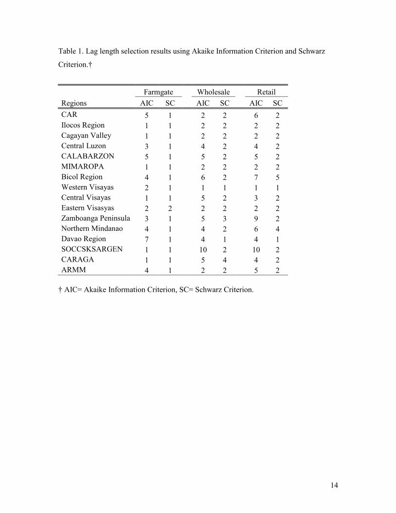
are considered. Starting with the maximum lag length of 12, the optimal lag is chosen on

the basis of the AIC and SC criterion. Table 1 shows the optimum lag length on farm

gate, retail and wholesale price series for all 16 regions. For almost all regions, the

optimal lag length is 1 month for all farm gate series. For retail and wholesale price series

the optimal lag length is 2 months in most of the regions.

[Table 1 about here]

After the determination of optimal lag length, we proceed to test for stationarity on series

at the farm gate, retail and wholesale. Table 2a shows results for stationarity test using

3 All estimations are performed with JMulti. It is an interactive software for time series analysis. More

information about can be obtained at http://www.jmulti.de/ 4 Peso is the currency used in the Philippines. 1 USD = 40 PhP.

9

ADF test. For the farm gate prices, the majority of regional series were found to be

stationary in levels. This is consistent with pricing theory which would suggest that

nominal cash commodity prices should be stationary around long-run production costs

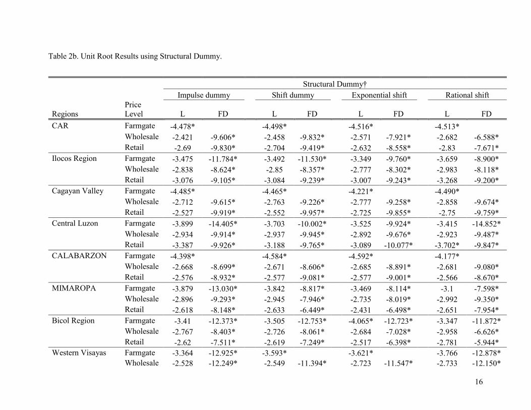
(Wang and Tomek, 2007). In contrast all retail and wholesale price series were found to

be I(1). Results of unit root tests with structural breaks are presented in table 2b. First of

all, one or two structural breaks were indentified in several instances. Second, results

seem to show similar patterns as the ADF results. The majority of farm gate price series

are I(0), while most of the series for retail and wholesale prices are I(1).

[Table 2a about here]

[Table 2b about here]

Following the procedure described in the methodology the null hypothesis of linear

model versus non-linear TV-STAR model was tested for all series at the different levels.

In cases where a non-linear STAR model is detected, the procedure also allows

estimation of the model with the appropriate functional form for the transition function.

In all cases the transition variable is assumed to be t, (as in Lin and Terasvirta, 1994) and

the function G allows a smooth transition across the endogenously defined regimes.

Results are presented in Table 3. It is interesting to notice that in all regions a non-linear

STAR-type dynamic is observed either for farm gate price, retail price, and wholesale

price or at all 3 levels. The majority of series exhibiting TV-STAR-types nonlinearity

have a logistic functional form (LSTAR1). The LSTAR1 type of nonlinearity

characterizes asymmetric price dynamic with regime of low and high values separated by

a smooth transition band.

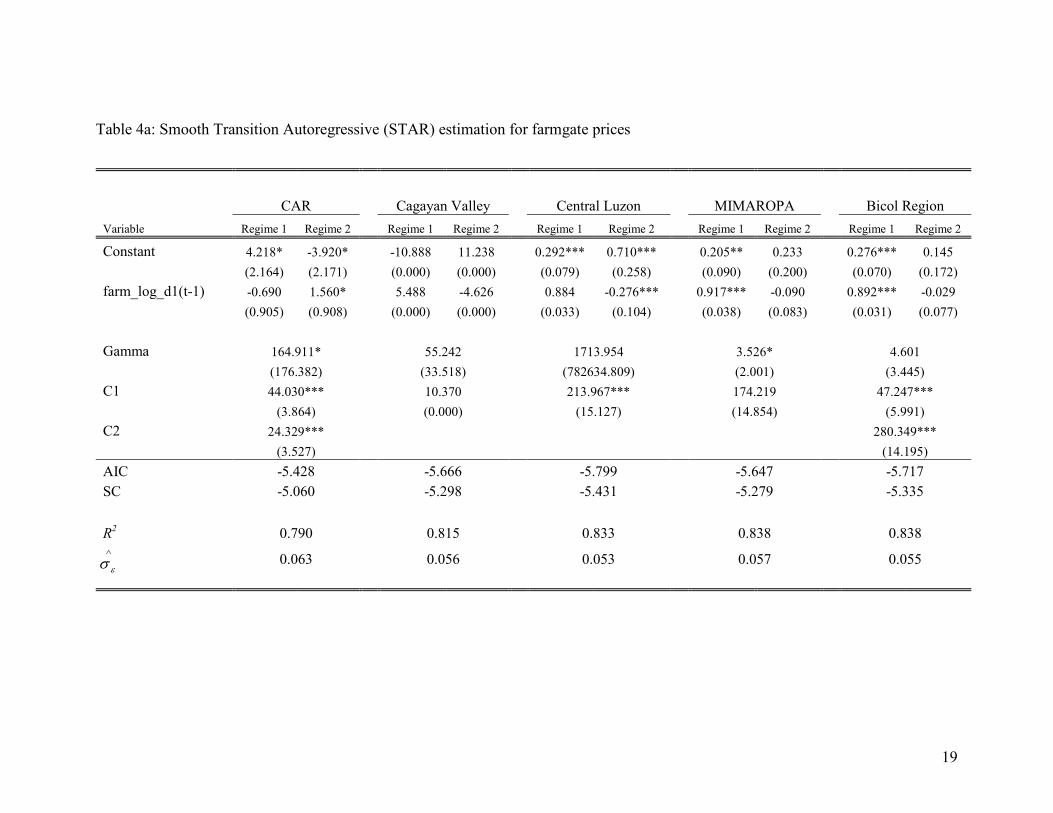
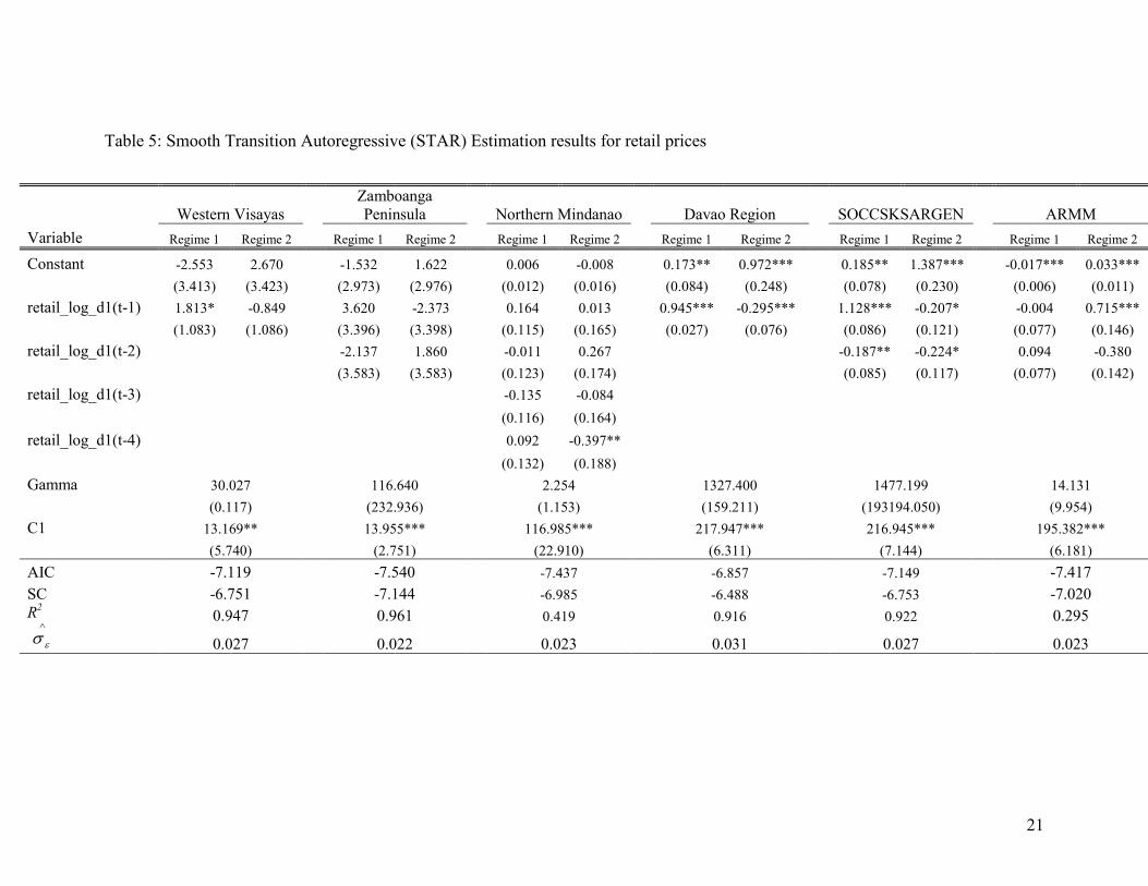
For the regions for which a STAR-type non-linearity was detected, we proceed to

the estimation of parameters as described in equation (6). Results are presented in Tables

4, 5 and 6. After estimation of these models, we also proceeded to their evaluation by

testing for the presence of additive nonlinearity and for parameter constancy. In almost

all cases no remaining nonlinearity was detected. Also, the null hypothesis of parameter

constancy was rejected in almost all cases with few exceptions. However in some

instances, the computed Gamma parameter appears to be quite high with large standard

10

errors. This was observed for example in the farm gate prices of central Luzon, the retail

price of Davao and SOCCSKSARGEN, the wholesale prices of Davao, CARAGA and

ARMM. For the price series where LSTR1 is found to be appropriate, the large value of

gamma indicates that the two regimes identified have equal variance. However, for

LSTR2, the large value of gamma indicates that there are 3 regimes (2 identical outer

regimes and a mid-regime).

It is interesting to observe that the LSTAR1 form of nonlinearity has been

predominant at the farm gate level. This could be due to the seasonal and cyclical nature

of rice production or weather influence. The regular intervention of the government in the

form of NFA stock could also be the source of the observed nonlinearity. The sources of

the observed nonlinearity warrant further investigation.

[Table 4 about here]

[Table 5 about here]

[Table 6 about here]

Conclusion

This paper investigates nonlinear dynamics in rice prices in 16 regions in the

Philippines at three levels: farm gate, wholesale and retail using A Smooth Transition

Autoregressive time series approach. Results show strong evidence of nonlinearity in the

price dynamics, in particular farm gate price dynamics are best characterized by a logistic

STAR process with two distinct regimes. This study is a work in progress and our results,

although important, represent only the preliminary step of our overall research goal –

namely to examine the sources of nonlinearity in Philippine rice price dynamics. We have

alluded to possible causes of rice price nonlinearities (e.g. government intervention,

periodic shocks in international rice market, and episodic weather effects), and the natural

extension to this paper is to investigate the specific potential sources of nonlinearity.

11

References

Bernard, J. C., & Willett, L. S. (1996). Asymmetric price relationships in the U.S. broiler

industry. Journal of Agricultural and Applied Economics, 28(2), 279-289.

Boyd, M. S., and Brorsen, B. W. (1988). Price asymmetry in the US pork marketing

channel. North Central Journal of Agricultural Economics, 10, 103-109.

Frey, G., & Manera, M. (2007). Econometric models of asymmetric price transmission.

Journal of Economic Surveys, 21(2), 349-415.

Girapunthong , N., VanSickle, J. J., & Renwick A. (2004). Price Asymmetry in the

United States fresh tomato market. Journal of Food Distribution, 34, 51-59.

Goodwin, B. K., & Holt, M. T. (1999). Price transmission and asymmetric adjustment in

the U.S. beef sector. American Journal of Agricultural Economics, 81(3), 630-

637.

Griffith, G. R., & Piggott, N. E. (1994). Asymmetry in beef, lamb and pork farm-retail

price transmission in Australia. Agricultural Economics, 10(3), 307-316.

Hassouneh, I., Serra, T., & Gil, J. M. (2010). Price transmission in the Spanish bovine

sector: the BSE effect. Agricultural Economics, 41(1), 33-33.

Hassouneh, I. von Cramon-Taubadel, S. & Gil, J.M. (2012). Recent developments in the

econometric analysis of price transmission. Working Paper No. 2, Transparency

of Food Pricing.

Holt, M., & Balagtas, J. (2009). Estimating structural change with smooth transition

regressions: an application to meat demand. American Journal of Agricultural

Economics, 91(5), 1424-1424.

Holt, M. T., & Craig, L. A. (2006). Nonlinear dynamics and structural change in the U.S.

hog-corn cycle: a time-varying STAR approach. American Journal of

Agricultural Economics, 88(1), 215-233.

Kinnucan, H. W., & Forker, O. D. (1987). Asymmetry in farm-retail price rransmission

for major dairy products. American Journal of Agricultural Economics, 69(2),

285-292.

Lin, C. F. J., & Teräsvirta, T. (1994). Testing the constancy of regression parameters

against continuous structural change. Journal of Econometrics,62(2), 211-228.

12

Lutkepohl, H. (2004). “Univariate Time Series Analysis” in H. Lütkepohl, and M.

Krätzig, (eds) Applied time series econometrics. Cambridge, UK: Cambridge

University Press.

Mainardi, S. (2001). Limited arbitrage in international wheat markets: threshold and

smooth transition cointegration. The Australian Journal of Agricultural and

Resource Economics, 45(3), 335-335.

Matriz, M.J. (2008). Price transmission mechanism in the Philippine rice industry.

Unpublished thesis. Master of Science in Agricultural and Resource Economics.

University of Delaware

Parrott, S. D., Estwood, D. B., & Brooker, J. R. (2001). Testing for symmetry in price

transmission: an extension of the Shiller lag structure with an application to fresh

tomatoes. Journal of Agribusiness, 19, 35- 49.

Peri, M., & Baldi, L. (2010). Vegetable oil market and biofuel policy: An asymmetric

cointegration approach. Energy Economics, 32(3), 687-693.

Reeder, M. M. (2000). Asymmetric prices: implications on trader’s market power in the

Philippine rice. Journal of Philippine Development, 49, 49-69.

Reitz, S., & Westerhoff, F. (2007). Commodity price cycles and heterogeneous

speculators: a STAR–GARCH model. Empirical Economics, 33(2), 231-244.

Romain, R., Doyon, M., & Frigon, M. (2002). Effects of state regulations on marketing

margins and price transmission asymmetry: Evidence from the New York City

and upstate New York fluid milk markets. Agribusiness, 18(3), 301-315.

Serra, T., & Goodwin, B. K. (2003). Price transmission and asymmetric adjustment in the

Spanish dairy sector. Applied Economics, 35(18), 1889-1899.

Shively, G. E. (1996). Food Price Variability and Economic Reform: An ARCH

Approach for Ghana. American Journal of Agricultural Economics, 78(1), 126-

136.

Terasvirta, T. (2004). “Smooth Transition Regression Modelling” in H. Lütkepohl, and

M. Krätzig, (eds) Applied time series econometrics. Cambridge, UK: Cambridge

University Press.

Terasvirta, T. and Anderson, H.M. (1992). “Characterizing Nonlinearities in Business

Cycles Using Smooth Transition Autoregressive Models” Journal of Applied

Econometrics 7:119–136.

Ubilava, D. (2012). Modeling nonlinearities in the U.S. soybean‐to‐corn price ratio: a

smooth transition autoregression approach. Agribusiness, 28(1), 29-41.

13

Ubilava, D., & Holt, M. (2013). El Niño southern oscillation and its effects on world

vegetable oil prices: assessing asymmetries using smooth transition models.

Australian Journal of Agricultural and Resource Economics, 57(2), 273-297.

Van Dijk, D., Terasvirta, T and Franses, P.H. (2002). “Smooth Transition Autoregressive

Models: A Survey of Recent Developments” Econometrics Review 21:1–47.

Vavra, P., & Goodwin, B. K. (2005). Analysis of price transmission along the food chain.

OECD Directorate for Food, Agriculture and Fisheries, OECD Food, Agriculture

and Fisheries Working Papers: 3.

Von Cramon-Taubadel, S. (1998). Estimating Asymmetric Price Transmission with the

Error Correction Representation: An application to the German Pork Market.

European Review of Agricultural Economics, 25(1), 1-18.

Von Braun, J. & Tadesse, G. (2012). Global Food Price Volatility and Spikes: An

Overview of Costs, Causes, and Solutions. Policy No. 161, ZEF-Discussion

Papers on Development. University of Bonn

Wang, D., & Tomek, W. G. (2007). Commodity prices and unit root tests.American

Journal of Agricultural Economics, 89(4), 873-889.

Ward, R. W. (1982). Asymmetry in retail, wholesale, and shipping point pricing for fresh

vegetables. American Journal of Agricultural Economics, 64(2), 205-212.

Worth, T. (2000). The FOB-retail price relationship for selected fresh vegetables.

Zhang, P., Fletcher, S. M., & Carley, D. H. (1995). Peanut price transmission asymmetry

in peanut butter. Agribusiness, 11(1), 13-20.

14

Table 1. Lag length selection results using Akaike Information Criterion and Schwarz

Criterion.†

Farmgate Wholesale Retail

Regions AIC SC AIC SC AIC SC

CAR 5 1 2 2 6 2

Ilocos Region 1 1 2 2 2 2

Cagayan Valley 1 1 2 2 2 2

Central Luzon 3 1 4 2 4 2

CALABARZON 5 1 5 2 5 2

MIMAROPA 1 1 2 2 2 2

Bicol Region 4 1 6 2 7 5

Western Visayas 2 1 1 1 1 1

Central Visayas 1 1 5 2 3 2

Eastern Visasyas 2 2 2 2 2 2

Zamboanga Peninsula 3 1 5 3 9 2

Northern Mindanao 4 1 4 2 6 4

Davao Region 7 1 4 1 4 1

SOCCSKSARGEN 1 1 10 2 10 2

CARAGA 1 1 5 4 4 2

ARMM 4 1 2 2 5 2

† AIC= Akaike Information Criterion, SC= Schwarz Criterion.

15

Table 2a. Results Unit Root testing with ADF.

Regions

ADF Test Statistic†

Farmgate Wholesale Retail

L FD L FD L FD

CAR -4.375* -2.856 -9.902* -2.814 -9.675*

Ilocos Region -3.371 -11.755* -3.019 -8.576* -3.097 -8.992*

Cagayan Valley -4.547* -2.877 -9.426* -2.76 -9.601*

Central Luzon -3.894 -14.102* -2.909 -9.648* -3.443 -9.768*

CALABARZON -4.209* -2.622 -8.899* -2.535 -8.879*

MIMAROPA -3.957 -13.481* -2.91 -9.199* -2.584 -8.064*

Bicol Region -4.145* -2.982 -8.272* -2.6 -7.260*

Western Visayas -3.748 -12.688* -2.769 -12.223* -2.521 -12.459*

Central Visasyas -5.203* -3.132 -8.834* -2.948 -8.632*

Eastern Visasyas -4.445* -2.71 -8.972* -2.816 -9.678*

Zamboanga Peninsula -4.482* -3.955 -12.604* -2.474 -10.480*

Northern Mindanao -4.305* -3.299 -10.560* -2.393 -7.636*

Davao Region -4.399* -3.469 -11.275* -3.437 -10.794*

SOCCSKSARGEN -3.813 -13.584* -3.545 -13.584* -3.771 -10.725*

CARAGA -4.741* -2.781 -9.102* -3.468 -9.963*

ARMM -6.034* -2.469 -9.007* -2.656 -8.409*

* Indicates rejection of null hypothesis of non-stationarity or unit roots at 1% level.

† L indicates series in level, FD first differenced series

16

Table 2b. Unit Root Results using Structural Dummy.

Structural Dummy†

Impulse dummy Shift dummy Exponential shift Rational shift

Regions

Price

Level L FD L FD L FD L FD

CAR Farmgate -4.478* -4.498* -4.516* -4.513*

Wholesale -2.421 -9.606* -2.458 -9.832* -2.571 -7.921* -2.682 -6.588*

Retail -2.69 -9.830* -2.704 -9.419* -2.632 -8.558* -2.83 -7.671*

Ilocos Region Farmgate -3.475 -11.784* -3.492 -11.530* -3.349 -9.760* -3.659 -8.900*

Wholesale -2.838 -8.624* -2.85 -8.357* -2.777 -8.302* -2.983 -8.118*

Retail -3.076 -9.105* -3.084 -9.239* -3.007 -9.243* -3.268 -9.200*

Cagayan Valley Farmgate -4.485* -4.465* -4.221* -4.490*

Wholesale -2.712 -9.615* -2.763 -9.226* -2.777 -9.258* -2.858 -9.674*

Retail -2.527 -9.919* -2.552 -9.957* -2.725 -9.855* -2.75 -9.759*

Central Luzon Farmgate -3.899 -14.405* -3.703 -10.002* -3.525 -9.924* -3.415 -14.852*

Wholesale -2.934 -9.914* -2.937 -9.945* -2.892 -9.676* -2.923 -9.487*

Retail -3.387 -9.926* -3.188 -9.765* -3.089 -10.077* -3.702* -9.847*

CALABARZON Farmgate -4.398* -4.584* -4.592* -4.177*

Wholesale -2.668 -8.699* -2.671 -8.606* -2.685 -8.891* -2.681 -9.080*

Retail -2.576 -8.932* -2.577 -9.081* -2.577 -9.001* -2.566 -8.670*

MIMAROPA Farmgate -3.879 -13.030* -3.842 -8.817* -3.469 -8.114* -3.1 -7.598*

Wholesale -2.896 -9.293* -2.945 -7.946* -2.735 -8.019* -2.992 -9.350*

Retail -2.618 -8.148* -2.633 -6.449* -2.431 -6.498* -2.651 -7.954*

Bicol Region Farmgate -3.41 -12.373* -3.505 -12.753* -4.065* -12.723* -3.347 -11.872*

Wholesale -2.767 -8.403* -2.726 -8.061* -2.684 -7.028* -2.958 -6.626*

Retail -2.62 -7.511* -2.619 -7.249* -2.517 -6.398* -2.781 -5.944*

Western Visayas Farmgate -3.364 -12.925* -3.593* -3.621* -3.766 -12.878*

Wholesale -2.528 -12.249* -2.549 -11.394* -2.723 -11.547* -2.733 -12.150*

17

Retail -2.296 -12.427* -2.323 -10.576* -2.302 -8.861* -2.498 -8.1400*

Central Visasyas Farmgate -4.718* -4.483* -4.175* -4.177*

Wholesale -3.097 -8.900* -3.121 -8.810* -3.16 -8.816* -3.242 -9.003*

Retail -2.926 -8.706* -2.924 -8.879* -3.002 -7.566* -3.053 -6.860*

Eastern Visasyas Farmgate -3.940* -4.335* -4.365* -4.284*

Wholesale -2.375 -9.057* -2.416 -9.056* -2.75 -8.987* -2.879 -9.362*

Retail -2.572 -8.218* -2.659 -8.168* -2.706 -9.623* -2.735 -9.792*

Zamboanga

Peninsula Farmgate

-4.079* -4.581* -4.610* -4.496*

Wholesale -3.759* -3.911* -3.989* -4.016*

Retail -2.379 -9.448* -2.412 -8.854* -2.49 -10.391* -2.516 -10.288*

Northern Mindanao Farmgate -3.549 -13.542* -3.305 -13.562* -4.253* -4.388*

Wholesale -3.309 -9.755* -3.283 -10.718* -3.213 -10.702* -3.26 -9.330*

Retail -2.235 -7.421* -2.294 -7.489* -2.249 -6.114* -2.456 -5.845*

Davao Region Farmgate -4.154* -4.028* -4.398* -4.363*

Wholesale -3.31 -11.082* -3.346 -11.569* -3.357 -10.517* -3.486 -9.996*

Retail -3.393 -10.968* -3.446 -10.987* -3.235 -10.884* -3.481 -10.358*

SOCCSKSARGEN Farmgate -3.746* -3.895* -3.078 -7.456* -3.154 -13.278*

Wholesale -3.183* -3.300* -3.493 -10.871* -3.578*

Retail -3.393 -10.941* -3.446 -10.976* -3.235 -10.872* -3.481 -10.216*

CARAGA Farmgate -4.120* -4.308* -4.770* -4.894*

Wholesale -2.457 -8.793* -2.436 -9.292* -2.566 -6.857* -2.688 -6.405*

Retail -3.114 -10.169* -3.021 -9.986* -3.007 -10.219* -3.47 -9.930*

ARMM Farmgate -5.131* -5.688* -6.863* -6.583*

Wholesale -2.623 -8.327* -2.609 -7.574* -2.413 -7.733* -2.718 -9.057*

Retail -2.763 -8.295* -2.729 -8.692* -2.729 -8.508* -2.838 -8.397*

* Indicates rejection of null hypothesis of unit roots at 1%. † L indicates series in

level, FD first differenced series

18

Table 3. Test Results between Linear and STAR-type Nonlinearity

Regions Farm Wholesale Retail

CAR LSTAR2 Linear Linear Ilocos Region LSTAR2 Linear Linear Cagayan Valley LSTAR1 Linear Linear Central Luzon LSTAR1 Linear Linear CALABARZON Linear Linear Linear MIMAROPA Linear Linear Linear Bicol Region LSTAR2 Linear Linear Western Visayas LSTAR1 LSTAR1 LSTAR1 Central Visayas LSTAR1 Linear Linear Eastern Visayas LSTAR1 Linear Linear Zamboanga Peninsula Linear LSTAR1 Linear Northern Mindanao LSTAR1 Linear LSTAR1 Davao Region LSTAR1 LSTAR1 LSTAR1 SOCCSKSARGEN LSTAR1 LSTAR1 LSTAR1 CARAGA LSTAR2 LSTAR1 Linear ARMM Linear Linear LSTAR1

19

Table 4a: Smooth Transition Autoregressive (STAR) estimation for farmgate prices

CAR Cagayan Valley Central Luzon MIMAROPA Bicol Region

Variable Regime 1 Regime 2 Regime 1 Regime 2 Regime 1 Regime 2 Regime 1 Regime 2 Regime 1 Regime 2

Constant 4.218* -3.920* -10.888 11.238 0.292*** 0.710*** 0.205** 0.233 0.276*** 0.145

(2.164) (2.171) (0.000) (0.000) (0.079) (0.258) (0.090) (0.200) (0.070) (0.172)

farm_log_d1(t-1) -0.690 1.560* 5.488 -4.626 0.884 -0.276*** 0.917*** -0.090 0.892*** -0.029

(0.905) (0.908) (0.000) (0.000) (0.033) (0.104) (0.038) (0.083) (0.031) (0.077)

Gamma 164.911* 55.242 1713.954 3.526* 4.601

(176.382) (33.518) (782634.809) (2.001) (3.445)

C1 44.030*** 10.370 213.967*** 174.219 47.247***

(3.864) (0.000) (15.127) (14.854) (5.991)

C2 24.329*** 280.349***

(3.527) (14.195)

AIC -5.428 -5.666 -5.799 -5.647 -5.717

SC -5.060 -5.298 -5.431 -5.279 -5.335

R2

0.790 0.815 0.833 0.838 0.838

0.063 0.056 0.053 0.057 0.055

∧

εσ

20

Table 4b: Smooth Transition Autoregressive (STAR) estimation for farmgate prices (cont’d)

Western Visayas Central Visasyas Eastern Visasyas Northern Mindanao Davao Region SOCCSKSARGEN

Variable Regime 1 Regime 2 Regime 1 Regime 2 Regime 1 Regime 2 Regime 1 Regime 2 Regime 1 Regime 2 Regime 1 Regime 2

Constant 0.241 0.067 0.410** -0.019 0.379*** 0.222 0.334*** 0.014 0.289 0.060

-

17227.647 17227.999

(0.324) (0.385) (0.197) (0.229) (0.113) (0.253) (0.090) (0.159) (1.107) (1.181) (0.000) (0.000)

farm_log_d1(t-1) 0.951*** -0.082 0.821*** 0.012 0.525*** 0.015 0.859*** 0.001 0.854* 0.001 6603.183 0.456

(0.194) (0.216) (0.081) (0.094) (0.072) (0.138) (0.040) (0.068) (0.493) (0.524) (0.000) (0.405)

farm_log_d1(t-2) 0.307*** -0.105

(0.071) (0.136)

Gamma 1.474 7.482 28.007 26.662 1.112 0.456

(1.412) (4.972) (29.116) (29.709) (0.000) (0.405)

C1 12.326 43.707*** 199.054*** 155.674*** -75.535 -1974.857

(175.155) (9.645) (4.441) (6.604) (0.000) (1543.607)

AIC -5.959 -5.314 -5.246 -5.873 -5.613 -6.008

SC -5.590 -4.945 -4.850 -5.504 -5.244 -5.640

R2

0.874 0.740 0.655 0.838 0.730 0.873

0.048 0.067 0.069 0.051 0.058 0.047

∧

εσ

21

Table 5: Smooth Transition Autoregressive (STAR) Estimation results for retail prices

Western Visayas

Zamboanga

Peninsula Northern Mindanao Davao Region SOCCSKSARGEN ARMM

Variable Regime 1 Regime 2 Regime 1 Regime 2 Regime 1 Regime 2 Regime 1 Regime 2 Regime 1 Regime 2 Regime 1 Regime 2

Constant -2.553 2.670 -1.532 1.622 0.006 -0.008 0.173** 0.972*** 0.185** 1.387*** -0.017*** 0.033***

(3.413) (3.423) (2.973) (2.976) (0.012) (0.016) (0.084) (0.248) (0.078) (0.230) (0.006) (0.011)

retail_log_d1(t-1) 1.813* -0.849 3.620 -2.373 0.164 0.013 0.945*** -0.295*** 1.128*** -0.207* -0.004 0.715***

(1.083) (1.086) (3.396) (3.398) (0.115) (0.165) (0.027) (0.076) (0.086) (0.121) (0.077) (0.146)

retail_log_d1(t-2) -2.137 1.860 -0.011 0.267 -0.187** -0.224* 0.094 -0.380

(3.583) (3.583) (0.123) (0.174) (0.085) (0.117) (0.077) (0.142)

retail_log_d1(t-3) -0.135 -0.084

(0.116) (0.164)

retail_log_d1(t-4) 0.092 -0.397**

(0.132) (0.188)

Gamma 30.027 116.640 2.254 1327.400 1477.199 14.131

(0.117) (232.936) (1.153) (159.211) (193194.050) (9.954)

C1 13.169** 13.955*** 116.985*** 217.947*** 216.945*** 195.382***

(5.740) (2.751) (22.910) (6.311) (7.144) (6.181)

AIC -7.119 -7.540 -7.437 -6.857 -7.149 -7.417

SC -6.751 -7.144 -6.985 -6.488 -6.753 -7.020

R2 0.947 0.961 0.419 0.916 0.922 0.295

0.027 0.022 0.023 0.031 0.027 0.023

∧

εσ

22

Table 6: Smooth Transition Autoregressive (STAR) estimation results for wholesale prices.

Northern Mindanao Davao Region SOCCSKSARGEN CARAGA ARMM

Variable Regime 1 Regime 2 Regime 1 Regime 2 Regime 1 Regime 2 Regime 1 Regime 2 Regime 1 Regime 2

Constant 0.007 0.189 0.174** 1.355*** 0.248 0.030 0.206** 1.944*** -0.068 0.181

(0.107) (0.131) (0.078) (0.265) (0.201) (0.221) (0.082) (0.322) (0.114) (0.125)

wholesale_log_d1(t-1) 0.886*** 0.309** 0.946***

-

0.428*** 0.828*** 0.314 0.957*** -0.235* 1.022*** 0.197

(0.106) (0.131) (0.026) (0.084) (0.230) (0.243) (0.079) (0.135) (0.106) (0.132)

wholesale_log_d1(t-2) 0.111 -0.369*** 0.083 -0.312 0.085 0.047 -0.014 -0.242*

(0.110) (0.135) (0.221) (0.235) (0.110) (0.166) (0.111) (0.135)

wholesale_log_d1(t-3) -0.049 -0.415**

(0.109) (0.165)

wholesale_log_d1(t-4) -0.059 0.020

(0.078) (0.129)

Gamma 99.517 2087.260 8.958 1805.112 1551.767

(216.624) (11653925.32) (0.000) (2315592.94) (867004.82)

C1 74.757*** 218.009*** 48.208*** 215.035*** 72.976***

(2.117) (50.970) (10.240) (45.355) (13.495)

AIC -7.130 -6.843 -6.515 -7.198 -7.240

SC -6.735 -6.475 -6.119 -6.747 -6.845

R2

0.928 0.926 0.898 0.939 0.950

0.027 0.031 0.037 0.026 0.025

∧

εσ