Improved Processing of AIRSAR Data Based on the GeoSAR Processor

Scott Hensley*, Elaine Chapin, Adam Freedman and Thierry Michel

Jet Propulsion Laboratory, 4800 Oak Grove Drive Pasadena, California 91109. MS 300-235

ABSTRACT

AIRSAR is a versatile multi-mode and multi-frequency radar. The system is able to collect fully polarimetric data atthree frequencies, C, L and P-band, and interferometric data, C and L band, in both cross track and along trackconfigurations. Data may be collected using a variety of bandwidths from 20-80 MHz using either 8-bit signal quantization orusing a Block Floating Point Quantized mode like that employed by the SIR-C radar systems. Accurate processing of allthese modes into useful geophysical products requires a very flexible processor. Currently, AIRSAR employs a combinationof three processors to generate products each tailored to meet the requirements of a particular data product. As theseprocessors were developed over the course of two decades the level of processing fidelity and flexibility vary substantially.Over the last five years as part of the GeoSAR program we have been developing the next generation of airborneinterferometric and polarimetric processors that may be used to improve the quality of some of the AIRSAR data products. Inthis paper we describe several of the novel processing algorithms incorporated into the GeoSAR processor and indicate howthey might improve AIRSAR products.

Keywords: GeoSAR, interferometry, topography, mapping, DEM

1. INTRODUCTION

Under the GeoSAR Program JPL has developed an end-to-end dual frequency interferometric and polarimetric radarprocessor. The GeoSAR radar is a dual frequency radar that operates in the X and UHF bands. Both bands are interferometricand map simultaneously on the left and right sides of the aircraft. The radar employs on arbitrary waveform generator so thatnotched chirped waveforms of 80 or 160 MHz bandwidth may be used. Offset video sampling of the echo data is either in 8bit or Block Floating Point Quantized Format (BFPQ). In order to accommodate the flexible nature of the radar commandand collection geometry, as well as give the user maximal flexibility and control when processing data, a modular softwaredesign architecture was employed (sometimes at the expense of throughput).

Besides the hardware and mode flexibility of the radar several other considerations affected the design anddevelopment of the processor. These included maintainability, readability, memory usage and parallelizability. The GeoSARprocessing subsystem is a series of programs designed to process and calibrate radar interferometry data collected by theGeoSAR radar mapping instrument. The GeoSAR processing subsystem consists of following five major programssometimes with modification may be used to process AIRSAR data

1. Motion Measurement Processor to combine the motion measurement data and compute most of time varyingparameters which affect the processing.

2. X-band processor to generate digital elevation models (DEM) from X-band raw signal data.3. P-band processor to generate digital elevation models (DEM) from P-band raw signal data.4. Calibration Software for calibrating the X and P-band interferometric mapping radars.5. Radio Frequency Interference (RFI) removal software.

The interferometric portion of the processing is subdivided into two main programs, the Motion MeasurementProcessor (MMP) and the interferometric Processor, jurassicprok. The primary function of the MMP is to reformat andcondition time varying radar parameter data in manner suitable for jurassicprok, whereas jurassicprok takes data generated by

* *Correspondence: Email: sh@kaitak.jpl.nasa.gov , Phone: (818)-354-3322 , FAX: (818)-393-3077

the MMP coupled with radar raw signal data and generates strip map output files. The remainder of this paper willconcentrate on the interferometric processor. Information on RFI removal is discussed in the companion paper [6].

2. GeoSAR SYSTEM OVERVIEW

To understand some of the considerations that went into the design of the GeoSAR processor it is useful to have acursory overview of the GeoSAR system. The GeoSAR radar flies onboard a Gulfstream-II aircraft and is a dual-frequency(P- and X-band) interferometric Synthetic Aperture Radar (SAR), with HH and HV (or VV and VH) polarization at P-bandand VV polarization at X-band. The radar hardware onboard the Gulfstream-II aircraft is supplemented with a Laser-BaselineMeasurement System (LBMS) which provides real-time measurements of the antenna baselines in platform based coordinatesystem which is tied to onboard Embedded GPS/INU (EGI) Units. GeoSAR maps a 20-km swath by collecting two 10-kmswaths on the right and left sides of the plane as shown in Figure 1.

Figure 1. GeoSAR collects 10 km swaths simultaneously on both left and right sides of the aircraft at both X and P-bands.

The P-band antenna system is mounted in the port and starboard wingtip pods providing a long antenna-baseline of about 20meters. X-band antennas are mounted in pairs under the wings with an antenna-baseline of 2.5 meters. Radar operations arecontrolled by a command disk generated preflight by the Mission Planning Software. Real-time data collection is controlledin-flight via an Automatic Radar Controller (ARC) that sets data collection windows, performs Built-In Test (BIT’s) beforeand after each datatake, and automatically turns the radar on and off during a data acquisition. Raw radar data is recorded onhigh-density digital tape recorders for subsequent, post-flight processing. The onboard data collection via the AutomaticRadar Controller also records navigation data from the aircraft’s GPS/INU system, the laser-based antenna-baselinemeasurement system, and raw signal data from X- and P-band radars. Table I gives a summary of the main systemparameters.

Table 1. GeoSAR System Parameters

Parameter P-Band Value X-Band Value

Peak Transmit Power 4 kW 8 kW

Bandwidth 80/160 MHz 80/160 MHz

Pulse Length 40 µs 40 µs

Antenna Gain 11 dBi 26.5 dBi

Look Angle Range 22° to 60° 22° to 60°

Center Frequency 350 MHz 9.755 MHz

Baseline Length 20 m and 40 m 2.6 m or 5.2 m

Baseline Tilt Angle 0° 0°

Platform Altitude5,000 m to10,000 m

5,000 m to10,000 m

3. PROCESSOR DESCRIPTION

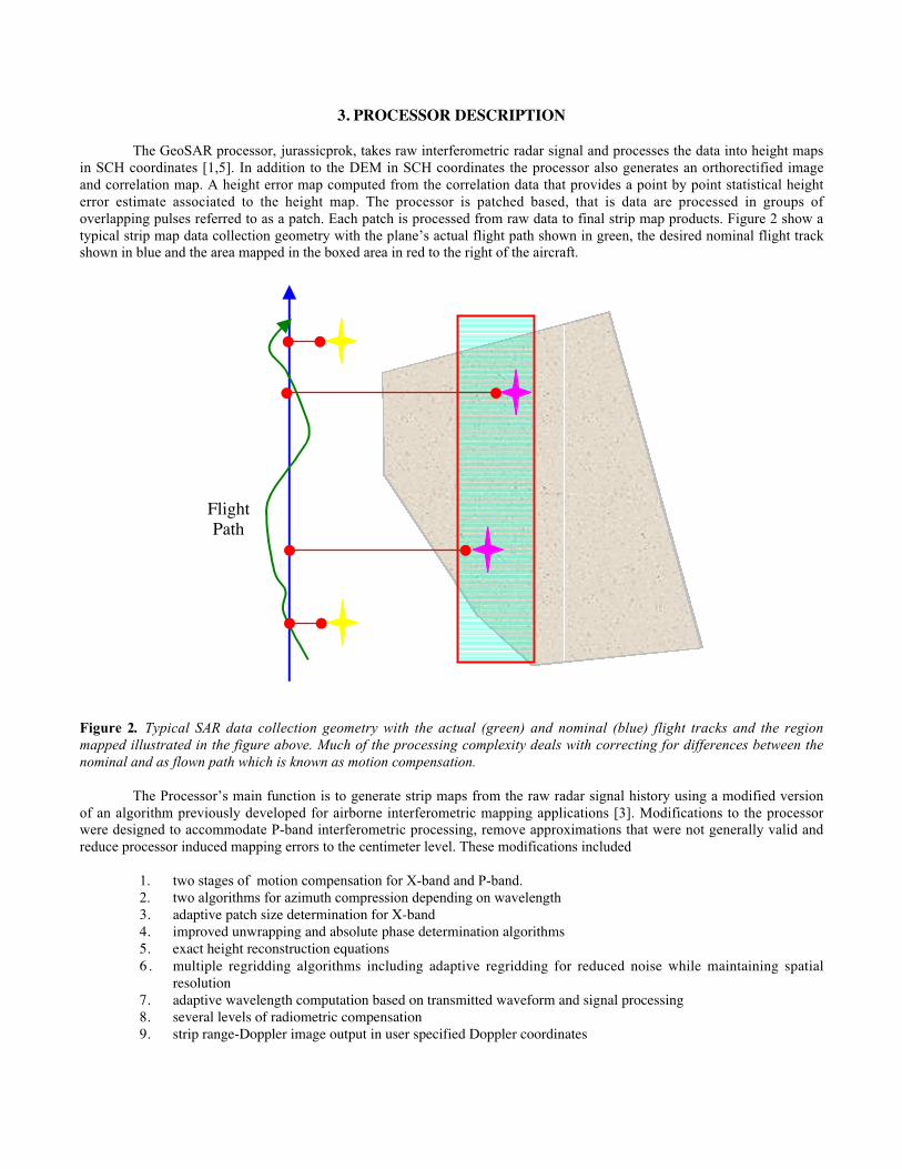
The GeoSAR processor, jurassicprok, takes raw interferometric radar signal and processes the data into height mapsin SCH coordinates [1,5]. In addition to the DEM in SCH coordinates the processor also generates an orthorectified imageand correlation map. A height error map computed from the correlation data that provides a point by point statistical heighterror estimate associated to the height map. The processor is patched based, that is data are processed in groups ofoverlapping pulses referred to as a patch. Each patch is processed from raw data to final strip map products. Figure 2 show atypical strip map data collection geometry with the plane’s actual flight path shown in green, the desired nominal flight trackshown in blue and the area mapped in the boxed area in red to the right of the aircraft.

Figure 2. Typical SAR data collection geometry with the actual (green) and nominal (blue) flight tracks and the regionmapped illustrated in the figure above. Much of the processing complexity deals with correcting for differences between thenominal and as flown path which is known as motion compensation.

The Processor’s main function is to generate strip maps from the raw radar signal history using a modified versionof an algorithm previously developed for airborne interferometric mapping applications [3]. Modifications to the processorwere designed to accommodate P-band interferometric processing, remove approximations that were not generally valid andreduce processor induced mapping errors to the centimeter level. These modifications included

1. two stages of motion compensation for X-band and P-band.2. two algorithms for azimuth compression depending on wavelength3. adaptive patch size determination for X-band4. improved unwrapping and absolute phase determination algorithms5. exact height reconstruction equations6. multiple regridding algorithms including adaptive regridding for reduced noise while maintaining spatial

resolution7. adaptive wavelength computation based on transmitted waveform and signal processing8. several levels of radiometric compensation9. strip range-Doppler image output in user specified Doppler coordinates

Reference Path

FlightPath

MappingArea

StripMap

Figure 3. Block diagram of the GeoSAR interferometric processor.

A block diagram for the GeoSAR topographic processor (called jurassicprok) is given in Figure 3. The processor ispatched based, that is the data to be processed is subdivided into overlapping regions called patches. Patch size variesdepending on frequency. This size of a patch is primarily driven be two factors. First, the need to maintain certain dataproducts in memory as well the need to have the Doppler centroid of the data approximately constant within the patch limitsthe size of a patch.. For longer wavelengths the need to have full synthetic aperture (16 km for P-band) forces the processorto handle very large patches. For machines where large amounts of RAM are not available the processor incorporated severalmemory saving features whereby some intermediate products could be written to disk. The green shaded area shows theprocessing done for each patch and blue boxed area shows in internal loop where small blocks pulse data are rangecompressed and presummed to save memory. A brief description of each of the major processing steps is given followed bymore detailed information in the subsequent subsections.

The first processing step is decoding the byte data, followed by range compression for each of the twointerferometric channels and then any polarimetric channels. Using the aircraft motion information obtained by the onboardaircraft motion measurement subsystem, which for GeoSAR consists of INUs, DGPS, and a laser baseline metrologysubsystem, the data are compensated for perturbations from the nominal flight track in the motion compensation modules.

X-band Data

X-band data is processed using a range-Doppler image formation algorithm. A brief outline of the processing stepsis described here. Raw data is range compressed using FFTs to carry out the convolution with the range reference function.The waveform for X-band is a simple down chirp with bandwidth of 80 or 160 MHz. The range reference functions areslightly different to accommodate the slight timing offsets between the two channels.

Subsequent to range compression the data are presummed to the grid specified in the Time Varying Parameter File(TVP File), generated by the MMP, that for X-band data has a nominal along track (S spacing) of .65 m. First stage motion

Jurassicprok

read pcf

jurassic_open

fill_sinc

Read Input Data

map setup

Begin Patch Loop

compute_patchdata

fill sinc

Loop on channels

copy presum save data

RAM Copydisk read

loop on presum blocks

rangecom

presum

mocom

azcomp_r azcomp_w

mocomp_co mocompI

LowMemor

BanX P

form_int in

blocks

apply caltone

intf filt

form_in

unw rt

inverse_mocom

abs_phas

height_recon

mapbuf_manager

regrid data

write ann

LowMemor

reske

antgain

compensation is applied to the best fit line that is parallel to a global reference track for each of the two channels. That is tosay the motion compensation line is optimized for each channel individually. Also, during motion compensation the drycomponent of atmosphere is compensated using a simple exponential model for the index of refraction so that the ranges inthe imagery are approximately the Euclidean distance from the platform to target. Magnitude of the effect is a function ofrange and varies from 2-3 m.

Azimuth compression uses a standard range-Doppler processing algorithm, however the Doppler for each channel isslightly different to insure highly accurate azimuth registration between the two channels. This Doppler difference is aconsequence of the wavenumber shift between the two interferometric channels that results when the baseline length is notequal to zero. Weighting of the azimuth reference function is a cosine on a pedestal with a use specified pedestal height.

Patch sizes for X-band may vary along track. The processor uses a nominal X-band patch size of 4096 presummedrange lines of which 3072 are valid after azimuth compression. However, if the aircraft attitude variation is deemed excessivefor this patch size (Doppler variation exceeds a specified fraction of the azimuth bandwidth) then the processor automaticallyreduces the patch size by half to 2048 presummed range lines which produces 1024 valid lines after azimuth compression.

After azimuth compression the data are then motion compensated to a common global reference line. A cosine on apedestal range weighting is applied to each channel after motion compensation for sidelobe reduction and to trim non-overlapping portions of the range spectrum which optimizes interferometric correlation. The pedestal height for the rangeweighting function is a user specified value nominally set to .5 which results in an effective range resolution reduction of afactor of 1.5 and a range ISLR of approximately 20 dB.

P-band Processing

P-band data is processed using an w -k processing algorithm followed by a special second stage motioncompensation algorithm designed to accommodate the large synthetic aperture angles required for P-band. Raw data is rangecompressed using FFTs to carry out the convolution with the range reference function. The waveform for P-band is a notchedchirp waveform designed to meet the spectral restrictions imposed by the NTIA. The notched nature of the waveformrequired the processor to compensate for changes in the effective interferometric wavelength due to the waveform. This canbe quite large (greater than a 1 cm) and varies with range due to the range dependent spectral shift between the channels.

Presumming and first stage motion compensation are identical to the X-band case. Azimuth compression uses amodified w-k processing algorithm and both channels are processed to zero Doppler. Weighting of the azimuth referencefunction is a cosine on a pedestal with a use specified pedestal height. Since first stage motion compensation corrects for therange delta along the fan beam direction (a narrow beam approximation) the imagery is not well focused after the first stageof motion compensation, however the energy for each point is localized spatially. In order to improve the azimuth focus asecond stage of motion compensation is applied where the azimuth compressed data are broken into subpatches andtransformed into the 2-D Fourier domain [5]. For each subptach a “best fit plane” to a reference DEM is used for the motioncompensation surface and a phase screen and frequency shift are applied to the data. The data are then transformed back tothe spatial domain and are then focused in azimuth. The data are then reskewed to the fan beam plane squint geometry. Also,during second stage motion compensation range weighting is applied similar to that described for X-band.

Imagery at this stage has been corrected for the r2 dependent range effect, however the antenna pattern correctionhas NOT been applied. This is not done until the height reconstruction stage of processing. Also, because the data has beenmotion compensated to a common reference path this effectively flattens the interferometric fringes, i.e. the fringes due to theperpendicular component of the baseline changing with respect to a curved earth are removed. This aid in the unwrappingprocess by reducing the average fringe frequency.

One of the single-look complex (SLC) image pair is used as reference to form an interferogram, (combine_int), thatis obtained by multiplying the complex pixel value in the reference image by the complex conjugate of the correspondingpixel in the second image. The resulting patch interferogram is multi-looked, by spatially averaging the complex pixelscomplex in box about a given pixel, (this is the optimal phase estimation algorithm) to reduce the amount of phase noise(filt_int). After the multi-looked interferogram has been generated, the phase for each complex sample is computed. Note thatthe phase measurement is made modulo 2p. To generate a continuous height map, the two-dimensional phase field must beunwrapped, that is, the correct multiple of 2p must be added to the phase of each pixel so that the relative phase between the

pixels will be correct (unw_rt). After the unwrapping process, there is an overall constant multiple of 2p phase offset (thatmay be zero) that needs to be added to each pixel so that the phase will have the correct relationship (abs_phase). Estimatingthis overall phase constant is referred to as absolute phase determination. Subsequent to determining the absolute phase foreach pixel in the interferogram the three dimensional target location is determined (height_recon). In order to accuratelyposition the targets, an accurate baseline estimate is required. In addition phase corrections are applied to the interferometricphase to account for tropospheric effects. A relief map is generated by gridding the unevenly sampled 3-dimensional targetlocations in a natural coordinate system aligned with the flight path (SCH coordinates). The data are periodically written todisk when the height data from the multiple patches fill a circular buffer containing the final gridded data products(mabuf_manager).

3.1 Range Compression

In the range compression module raw signal data is decoded from either 8-bit or 4-bit block floating pointquantization (BFPQ) format to floating point. BFPQ is data compression algorithm used to reduce the 8-bit data output fromthe ADC to 4-bits. The algorithm is structured to preserve the original signal dynamic range by assigning an exponent andmantissa for each sample and reducing the data rate by forcing the exponent to be the same for a group of samples. Data isblocked into groups of 128 samples and an exponent for each block is assigned and each sample in the block is assigned a 4-bit mantissa. This decoding is done via a look up table. Range compression is done using the standard Fourier transformconvolution algorithm. A calibration tone that is normally injected into the returned echo data to track phase drift between thechannels is extracted and stored for use in computing the relative phase between the two interferometric channels. A phaseramp is applied to the reference function of the two channels to remove differential channel delay and correct for an overallphase constant.

3.2 Presumming and Azimuth Compression

Presumming resamples the pulse data from the natural pulse spacing to a uniform along track grid. A bandpass filteroperation that employs a weighted sinc kernel is used to resample the data. Data is presummed in small blocks (256 pulses)and the bandpass filter is updated on each block to accommodate Doppler variations along track. Presumming is also used toreduced the along track sampling rate and reduce noise thereby improving throughput and data quality.

3.3 Motion Compensation

Motion compensation is the process where the radar signal data are resampled from the actual path of the antenna toan idealized path called the reference path. To motion compensate the data the delta range, Dr, from the reference path to the

antenna location, d , along the line-of-sight vector, √lR , is computed a range and phase correction are applied to each sampleusing the expressions

D D Dr r f pl

rª ( ) =d hR ref, √ , ,l4

where r is the range, l is the wavelength, and href is the motion compensation reference height. Motion compensation is done

Figure 4. A range and phase correction equal to the range difference between the actual and desired path is applied to bothchannels is shown highlighted in blue.

r

rd

√lT

√lR

first to local reference paths for each antenna and then to a common reference path, as shown in Figure 5, which insures thedata are co-registered in range after image formation, applies the appropriate range spectral shift for a flat surface and flattensthe fringes. For P-band data a more sophisticated motion compensation algorithm is employed as was described above.Range weighting is done after motion compensation to reduce sidelobes and trim the non-overlapping portions of the rangespectra. Plots of the time domain range weighting function and the associated range impulse responses are shown in Figure 6for several values of h.

Figure 5. This figure shows the four possible reference path scenarios that can occur in mocomp. Color coding of flight lines(solid lines) and reference paths (dotted lines) is as follows: blue and red indicate transmit and receive on the same antenna,purple indicates transmit on one antenna receive on the other, green is used for common reference paths. Equations for thevarious reference line are indicated below where,

rRi , is the reference path for antenna i,

rLinu , is the best fit line to the INU

location over the patch that is parallel to the global reference, and rlanti

, is the leverarm from the INU to the ith antenna.

Antenna 1 is assumed to be the transmit antenna except for Ping-Pong situations where antenna 2 also transmits.

Figure 6. Graph of the time domain weights for h equal to 0 (red), .5 (green), .08 (blue), and 0 (black) with the associatedimpulse responses shown in the adjacent graph. Note the trade between sidelobe level and impulse response width.

Mocomp II Active Mocomp II Inactive

rr r

lr r

lR =

L T R

L T Ri

inu ant 1 1

inu ant 2 2

1

2

++

ÏÌÔ

ÓÔ

rr r

lr r

lrl

R L T R

L T Ri

inu ant 1 1

inu ant ant 1 2

1

1 2

=+

+ +( )ÏÌÔ

ÓÔ1

2

r r rl

rlR = L +

1

2inu ant ant1 2+( )

Ping-Pong Ping-PongSAT SAT

r r rl

rlR = L + inu

1

43

1 2ant ant+( )

3.4 Interferogram Formation and Filtering

One of the single-look complex image pair is used as reference to form an interferogram, that is obtained bymultiplying the complex pixel value in the reference image by the complex conjugate of the corresponding pixel in thesecond image. Noise reduction in the interferogram uses either a simple box car spatial filtering algorithm or for very toughscenes the power spectral filtering can be used. Box car filtering multi-looks the data by spatially averaging the complexpixels complex in box about a given pixel, (this is the optimal phase estimation algorithm) to reduce the amount of phasenoise The basic idea of power spectral filtering [3] is that in a small box the phase rate is nearly constant, as seen in Figure 7,so that the two dimensional Fourier transform will have a well defined peak at the spatial frequency of the local fringes asillustrated in Figure 7.

Figure 7. The local fringe rate looks nearly constant in a small box in areas of fast and slow fringes as indicated by thehighlighted regions. Inset shows Fourier transform is peaked at the local fringe rate.

Weighting the spectrum proportional to the amount of spectral power enhances the local fringe rate and reduces the noise.More precisely, if s(i,j) denotes the interferogram values, S(n,m), the 2D Fourier transform of s(i,j), and F, the Fouriertransform operator then the power spectral weighted spectrum sw(i,j) is given by

s (i, j) = w F- +( )1 1S m n ei S m n( , ) arg( ( , ))a

where a is the filter exponent. Note that a filter exponent of 0 does no filtering to the interferogram whereas a filter exponent

of 1 is quite heavy smoothing of the interferogram.

3.5 Unwrapping and Absolute Phase Determination

Phase unwrapping consists of determining the correct multiple of 2p to add to the phase of each point in aninterferogram such that the integrated phase along any closed path constant. Unwrapping uses an updated version of theresidue based unwrapping algorithm [4] (other options include least squares and network flow algorithms). The algorithm ispatched based so that in principle an infinitely long strip of data could be unwrapped. For each patch the correlation is used tomask out areas of low correlation. Residues are computed to determine points where phase discontinuities exist in theunwrapped phase. Residues are connected if a “tree growing process” to insure that the resulting phase can recovered withoutphase discontinuities. The tree growing algorithm uses “neutrons” based on intensity and phase slope to aid in selecting pathsto connect the residues. It can happen in the tree growing process that every point in the interferogram can not be connectedby a path to any other point without crossing a branch cut. Subregions in the interferogram that can be connected by acontinuous path without crossing a branch cut are called connected components. Phase continuity between patches is

preserved by retaining a line of phase values in the overlap region that is used to bootstrap the phase from one patch to thenext. If the phase variance of the phase values on the overlap line between the two patches on a connected component issmaller than a threshold the bootstrap is considered successful otherwise the correlation threshold is raised and anotherunwrapping attempt is made. If correlation threshold is raised to some maximum value without reducing the phase variancesufficiently the region discarded.

Trees (branch cuts) are used to connect residues and are lines (like branch cuts in complex analysis) that cannot becrossed during the phase unwrapping process without phase inconsistencies in the resulting phase field. There are two typesof residues, positive and negative charged, that must be connected in such a way that the net sum (charge) is zero. Growingof trees in the most difficult part of the unwrapping process. Tree selection is based in part on heuristic algorithms and treerealization depends on where the tree growing process is started. To aid the tree growing process neutrons, which have zerocharge, are introduced. Neutrons are used to guide the lines (branches) connecting the residues so that they align morenaturally with areas intrinsically difficult to unwrap. Intensity neutrons are designed to help tree growth in layover regions.The idea is layover occurs when slopes are near perpendicular to the line-of-sight and appear very bright in SAR imagery andhave lower correlation. By detecting points that are sufficiently bright and of low enough correlation compared to thebackground they can be used to guide tree growth as illustrated in Figure 8.

Figure 8. Neutrons are generated along bright lines to help tree growth particularly in layover regions. The image on the leftis a representative SAR image with the white line representing an area of layover. Positive residues are show in blue,negative residues in red, and neutrons in green. Areas that are bright compared to the background and low in correlation(image of left is the corresponding correlation image with green high and blue low correlation) are designated as intensityneutrons.

A point is designated as an intensity neutron if the following inequalities are satisfied

I i j I

i jT I

T

( , )

( , )

≥ +£

m sg g

where I(i,j), g(j,j) are the image intensity and correlation at point (i,j), I and sI are the mean and standard deviation of the

image intensity for the patch, and mT and gT are the user specified intensity and correlation neutron thresholds respectively.

After determining the relative phase between the pixels an overall constant multiple 2p of may need to be added tothe phase to reconstruct the height correctly. Determining this multiple 2 p of is called the absolute phase determinationproblem. Two algorithms for determining the absolute phase are included in jurassicprok. One method uses a low resolutionDEM and the other attempts to estimate the absolute phase directly from the data. Sometimes either of these algorithms mayfail and therefore the user is provided with the capability to adjust the processor determined absolute phase either globally oron a patch-by-patch basis. Absolute phase determination is not done on every patch if it is possible to use the unwrappedphase from the previous patch to determine the absolute phase. This process is called phase bootstrapping. Bootstrappingcompares the unwrapped phase along selected lines in the overlap region to determine the absolute phase constant for thenext patch. How closely this must be a multiple of 2 p is determined by the phase variance threshold a parameter whichspecified by the user.

Bootstrapping is the preferred method of determining the absolute phase for all patches after the first patch. Phase iscompared along a set of lines in the overlap region of two patches as shown in Figure 9. If the number of points on thebootstrap lines exceeds a threshold then the variance of the phase difference on the bootstrap lines is checked to see if it

exceeds the phase variance threshold. If the phase variance threshold is exceeded then the correlation threshold isincremented by a user specified amount and the unwrapping process is repeated. This continues until either the phasevariance threshold is not exceeded or the maximum correlation threshold (is reached. If the maximal correlation threshold isreached and the phase variance still exceeds the phase variance threshold then the region is marked as unwrappable.

Figure 9. Two consecutive patches after unwrapping are shown above. The blue line denotes a river or other dark featurethat could not be unwrapped. Patch N-1 has three connected components shown in green, yellow and red. The green and redconnected components do not intersect the overlap region from patch N-2 and thus the absolute phase could not bebootstrapped. For these regions jurassicprok uses the low resolution database to determine the ambiguity (if they exceed aminimum size). Patch N has two connected components shown in yellow and red. Notice the number of connectedcomponents can change from patch to patch. The dotted line is the bootstrap phase line. Note different processingparameters for each patch slightly alters the location of the bootstrap line. This is compensated for when computing thephase differences. The variance of the phase difference on the line is compared to the threshold to determine if bootstrappingis allowed.

3.6 Height Reconstruction and Regridding

Interferometric height reconstruction is the determination of a target’s position vector from known platformephemeris information, baseline information and interferometric phase. Prior to height reconstruction the interferometricphase altered during the motion compensation process is “restored” to the true phase as sensed by the antenna at the time thepoint was imaged, a process called inverse motion compensation. Correction for dry tropospheric effects on all of theinterferometric measurements (range, Doppler and interferometric phase) is made prior to height reconstruction. Certainaffects such as multi-path or switch leakage can result in systematic phase distortions that can affect the reconstructed heightin 1-10 m range. Provided the multi-path or switch leakage signal resulting in the phase distortions is stable then it can beremoved through the use of a phase screen. The phase screen applies a range dependent correction to the interferometricphase. After the phase and range have been corrected for atmosphere and systematic phase distortions the reconstructed targetposition vector, T , is obtained by solving for the intersection locus of the range sphere centered at the platform positionvector, P , the Doppler cone with generating axis given by the velocity vector, v , and cone angle a function of the targetDoppler centroid, f, and the phase hyperboloid where f is the interferometric phase, r is the range, b is the baseline vectorand l is the wavelength. The simultaneous set of equations is given by

P T

f v

bb

- =

=

= - + -ÊË

ˆ¯

ÊËÁ

ˆ¯̃

Ê

Ë

ÁÁ

ˆ

¯

˜˜

r

l

fp

lr

r r

2

21

21

21

2

, √

√,

l

l

Patch N-1 Patch N

}

{

By a clever choice of coordinate systems this non-linear set of equations can be readily solved in closed form.

After height reconstruction each unwrapped phase point consists of a triple of numbers, the SCH coordinates of thatpoint. This point does not necessarily lie on an output grid point. Position vectors are not uniformly distributed in the SCplane following height reconstruction and need to be resampled to a uniform output grid. This resampling process is calledregridding. The basic goal of DEM generation is to generate elevation measurements having the greatest possible accuracyand the highest possible spatial resolution. For a given measurement system a trade between accuracy and resolutionnormally is made in order to meet final application needs. Without a specified application metric that can be optimized thereis not a well defined “optimal” solution that balances resolution and accuracy. A set of quantitative measures of mappingperformance can be used to assess how resolution and accuracy are being traded off that coupled with qualitative measuresand application specialist evaluations used to determine the “best” regridding algorithm. Jurassicprok supports fourregridding algorithms, each with advantages and disadvantages, providing maximal flexibility in meeting varied customerrequirements.

The four interpolation or resampling algorithms implemented in jurassicprok and which listed in order of increasingcomputational complexity are:

Nearest neighbor - Fast and easy but shows some artifacts in shaded relief images.

Simplicial - Uses a plane passing through three points containing the point where interpolation is required. Thisalgorithm is reasonably fast and accurate and provides a minimal amount of noise reduction.

Convolutional - Uses a windowed Gaussian interpolation kernel that approximates the optimal prolate spheroidalweighting function for a specified bandwidth to obtain interpolated height values. This algorithm does a good jobreducing noise while maintaining height resolution.

First or second order surface fit - Uses the height data centered in a box about a given point and does a weightedleast squares surface fit. This is the only algorithm that uses local weights based on local covariance measurementsas part of the resampling process. This algorithm does a good job reducing noise while maintaining heightresolution.

Jurassicprok permits the use of different regridding algorithms for the primary strip map products, although in mostapplications the same algorithm will be used for all layers. The surface fit algorithm, which often yields the best heightresampling, does not do a very good job with the correlation and image layers. The convolutional yields good results for alllayers and requires less CPU resources than surface fitting. The other two algorithms are faster and are good choices whenfast final output in needed for checkout or for optimizing other processing parameters.

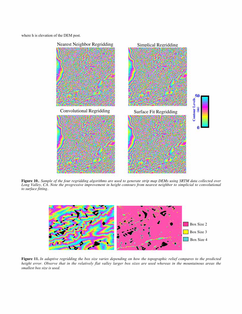
Figure 10 shows a comparison of the four regridding algorithms using SRTM data from Long Valley, CA. Note theprogressive improvement in height contours from nearest neighbor to simplicial to convolutional to surface fitting. One of theregridding features that can be used with either convolutional or surface fit regridding is adaptive regridding. In the adaptiveregridding process the amount of smoothing is adjusted depending on the amount of topographic relief compared to theintrinsic height measurement noise. The amount of smoothing is adjusted spatially by changing the box size used forregridding. The user selects a minimum, wmin, and maximum, wmax, allowed box size and the box size is adjusted betweenthese two values. Smaller box sizes smooth the data less than larger box sizes. Figure 11 shows an example where theadaptive regridding algorithm changes the box size that depends locally on the amount of topographic variation compared tothe height noise.

The orthorectified magnitude data is corrected for antenna pattern and range effects and scaled to giveradiometrically correct values. SCH coordinates (s,c,h) for a map pixel (sample, line) are obtained via the expression

s

c

h

S line s

C sample c

h

o post

o post

È

Î

ÍÍÍ

˘

˚

˙˙˙

=+ -

+ -È

Î

ÍÍÍ

˘

˚

˙˙˙

( )

( )

1

1

DD

where h is elevation of the DEM post.

Figure 10.. Sample of the four regridding algorithms are used to generate strip map DEMs using SRTM data collected overLong Valley, CA. Note the progressive improvement in height contours from nearest neighbor to simplicial to convolutionalto surface fitting.

Figure 11. In adaptive regridding the box size varies depending on how the topographic relief compares to the predictedheight error. Observe that in the relatively flat valley larger box sizes are used whereas in the mountainous areas thesmallest box size is used.

Nearest Neighbor Regridding Simplical Regridding

Convolutional Regridding Surface Fit Regridding

0

50

Con

tour

Lev

els

(m)

Box Size 2

Box Size 3

Box Size 4

3. 7 Radiometric Compensation

Although not a requirement for generating topographic maps the amplitude data are radiometrically corrected to aidin various scientific and classification studies. Radiometric correction is done in four steps. Compensation for the rangesquared amplitude reduction is applied immediately after range compression.. The elevation antenna pattern correction isapplied after height reconstruction when the precise look vector, including terrain effects, is known. Using the look vectorand the antenna geometry the precise antenna elevation angle can be computed. An option for correcting the radar backscatterfor the ground area is included in the processor. For many applications the corrected backscatter is a more useful quantity.Correction for the area projection factor, A, is applied during regridding using the equation below where A is the area the onthe ground responsible for the scattering, Dr and Ds are the range and along track resolution element dimensions respectively,and gc and gs are the cross track and along surface tilts as shown in Figure 12.

As

n n

s

I

c s

c s

= =-

-D D D D

S

r r g gq g g√ , √

sin ( )sin ( )

sin( )cos( )

1 2 2

Figure 12..To obtain a terrain corrected backscatter image the returned signal from a resolution element must be normalized by theground projected area of the resolution element. The area of the resolution element in the slant plane divided by the dot product of theterrain surface normal and the imaging normal gives the ground projected area. The dot product can be expressed in terms of the localterrain slopes and the look angle as indicated by above.

4. PROCESSING RESULTS

An example of data processed with AIRSAR data using the jurassicprok processor is data collected over OrangeCounty, California in 1999. Eight passes were collected, six were approximately east west aligned and two were collected onorthogonal flight lines to help removal any residual tilts in the mosaicking process. Adaptive convolutional regridding wasused to process this data and reduced the random point to point height noise from around 1.5 m to .5 m in the flat areas. Also,there are no patch boundary height discontinuities when data are processed using jurassicprok which can help for studieswhere the highest elevation accuracy is required.

√nS

√nI

Line of sightto resolution element

Ds

Dr

gc

Figure 13. This figure is a mosaic of processed TOPSAR data from a Orange County collection. Each color cycle used todepict elevation contours and represents 100 m of elevation change. Brightness in the image mask mosaic is derived from ashaded relief of the USGS DEM used to make the mask whereas in the TOPSAR mosaic it is the radar backscatter.

5. CONCLUSIONS

The GeoSAR interferometric was designed with efficient precision processing a major goal. The algorithms used arestate of the art and the front end offers the processing engineer a great deal of flexibility in how to process data. Usingjurassicprok to process AIRSAR is expected to improve the quality of interferometric data products in the near term andeventually polarimetric data products in the future.

ACKNOWLEDGMENTS

This paper was written at the Jet Propulsion Laboratory, California Institute of Technology, under contract with theNational Aeronautics and Space Administration. We would like to thank NIMA and DARPA for sponsorship of the GeoSARprogram and Dr. Mike Sapper who helped generate a number of the images contained in this paper.

REFERENCES

1 . P. Rosen, S. Hensley, I. Joughin, F. Li, S. Madsen, E. Rodriguez and R. Goldstein, “Synthetic Aperture RadarInterferometry,” Proceedings of the IEEE, vol. 88, no 3, March 2000

2. S. Madsen, H. Zebker, and J. Martin, “Topographic Mapping using radar interferometry: Processing Techniques,” IEEETrans. Geosci. Remote Sensing, vol. 31, pp. 246-256, 1993.

3. R. Goldstein and C. Werner, “Radar interferogram filtering for geophysical applications,” Geophysical Res. Lett., vol.25, no. 21, pp. 4035-4038, 1998.

4. R. Goldstein. H. Zebker and C. Werner, “Satellite Radar Interferometry: Two-dimensional phase unwrapping,” RadioSci., vol. 23, no. 4, pp. 713-720, 1988.

5 . Hensley. S., R. Munjy and P. A. Rosen, “Interferometric Synthetic Aperture Radar (IFSAR)”, Chapter 6, DigitalElevation Model Technologies and Applications: The DEM Users Manual, ASPRS, 2001.

6. Madsen, S., ‘Motion Compensation for UWB SAR”, IGARSS Proceedings 2001.

7. Le, C. and Hensley, S., ‘RFI Removal for AIRSAR Polarimetric Data”, Proceedings AIRSAR 2002 Conference.

Appendix: SCH Coordinates

Ellipsoid Coordinates

Provided below are the formulas and a couple examples for converting between SCH coordinates and WGS-84 XYZcoordinates. SCH is a spherical system aligned with the platform motion that is well suited to motion compensation yet hassimple exact expressions for converting to standard geographic coordinates as needed for precision mapping applications.

Geographic coordinates of a point are specified by the latitude, l, longitude q, and the height above the surfacealong the outward pointing normal to the earth’s surface. The earth’s surface for mapping and navigation purposes is mostcommonly modeled as ellipsoid of revolution about the earth’s spin axis. Two parameters are needed to specify the shape ofthe ellipse.

Latitude and longitude used is always the geodetic latitude and longitude as defined below. Note the equationsprovided below for converting between geographic and geocentric coordinates are approximate formulas that should beadequate for most applications. Exact formulas are available and can be substituted if necessary.

a

b

l

r e(l)

g

P

Figure A.1. Geometry of the ellipse.

Geodetic latitude is the angle between the unit normal to the surface and the plane perpendicular to the generatingaxis. Complete characterization of the shape of the generating ellipse of the ellipsoid can be done with two parameters, thelength of the semi-major axis, a, and the eccentricity, e, a measure of the oblateness of the ellipse. Eccentricity is be related tothe length of the semi-minor axis, b, by

b2 = a2(1 - e2)

The distance from a point p on the ellipsoid to the intersection of the unit normal to the surface at that point and the z axis,re(l), is a function of geodetic latitude given by

re(l) = a

1 - e2 sin2 l12

re(l) turns out to be related to the geometry of the surface, it is the radius of curvature in the east direction. The functions f

and g used to parameterize the ellipsoid are given by

f(l) = re(l) cos(l) , g(l) = re(l) (1 - e2) sin(l).

It is sometimes useful to relate the geocentric latitude, g, to the geodetic latitude, l. The relationship is

tan g = (1 - e2) tan l .

Another parameter often used to characterize the oblateness of an ellipse is the flattening, f, given by the relation

e2 = f (2 - f).

A standard ellipsoid often used in simulations is the WGS-84 ellipsoid that has equatorial radius a = 6378.137 km and e2 =.00669437999015.

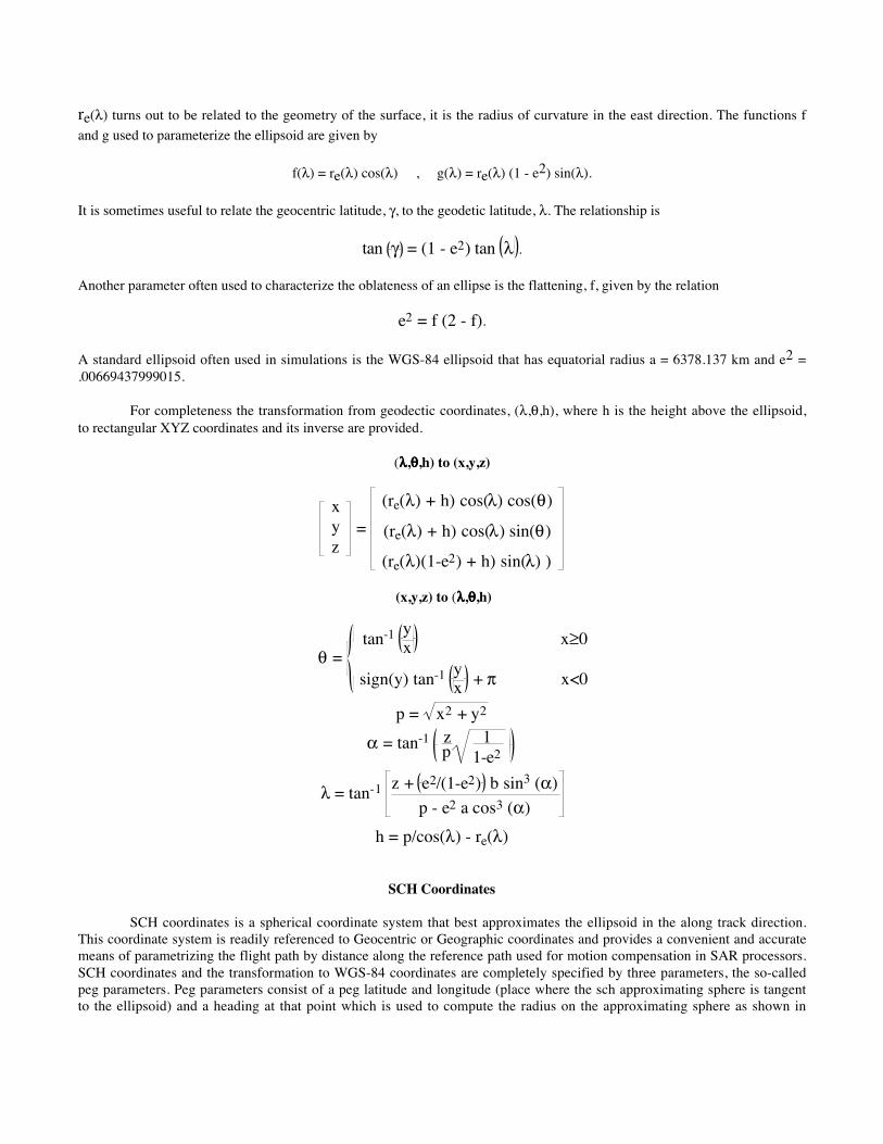
For completeness the transformation from geodectic coordinates, (l,q,h), where h is the height above the ellipsoid,to rectangular XYZ coordinates and its inverse are provided.

(llll,qqqq,h) to (x,y,z)

xyz

=

(re(l) + h) cos(l) cos(q)

(re(l) + h) cos(l) sin(q)

(re(l)(1-e2) + h) sin(l) )

(x,y,z) to (llll,qqqq,h)

q = tan-1

yx x≥0

sign(y) tan-1 yx + p x<0

p = x2 + y2

a = tan-1 zp1

1-e2

l = tan-1 z + e2/(1-e2) b sin3 (a)

p - e2 a cos3 (a)

h = p/cos(l) - re(l)

SCH Coordinates

SCH coordinates is a spherical coordinate system that best approximates the ellipsoid in the along track direction.This coordinate system is readily referenced to Geocentric or Geographic coordinates and provides a convenient and accuratemeans of parametrizing the flight path by distance along the reference path used for motion compensation in SAR processors.SCH coordinates and the transformation to WGS-84 coordinates are completely specified by three parameters, the so-calledpeg parameters. Peg parameters consist of a peg latitude and longitude (place where the sch approximating sphere is tangentto the ellipsoid) and a heading at that point which is used to compute the radius on the approximating sphere as shown in

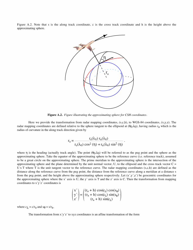
Figure A.2. Note that s is the along track coordinate, c is the cross track coordinate and h is the height above theapproximating sphere.

h

ra

Figure A.2. Figure illustrating the approximating sphere for CSH coordinates.

Here we provide the transformation from radar mapping coordinates, (s,c,h), to WGS-84 coordinates, (x,y,z). Theradar mapping coordinates are defined relative to the sphere tangent to the ellipsoid at (q0,l0), having radius ra which is theradius of curvature in the along track direction given by

ra = re(l0) rn(l0)

re(l0) cos2 (h) + rn(l0) sin2 (h) .

where h is the heading (actually track angle). The point (q0,l0) will be referred to as the peg point and the sphere as theapproximating sphere. Take the equator of the approximating sphere to be the reference curve (i.e. reference track), assumedto be a great circle on the approximating sphere. The prime meridian to the approximating sphere is the intersection of theapproximating sphere and the plane determined by the unit normal vector, U, to the ellipsoid and the cross track vector C =U x T where T is the unit tangent vector to the reference curve. The radar mapping coordinates (s,c,h) are defined as thedistance along the reference curve from the peg point, the distance from the reference curve along a meridian at a distance sfrom the peg point, and the height above the approximating sphere respectively. Let (x´,y´,z´) be geocentric coordinates forthe approximating sphere where the x´ axis is U, the y´ axis is T and the z´ axis is C. Then the transformation from mappingcoordinates to x´y´z´ coordinates is

x´y´z´

= (ra + h) cos(cl) cos(sq)(ra + h) cos(cl) sin(sq)

(ra + h) sin(cl)

where cl = c/ra and sq = s/ra.

The transformation from x´y´z´ to xyz coordinates is an affine transformation of the form

xyz

= MENUxyz Mx´y´z´

ENU x´y´z´

+ O

where O is a translation vector, Mbc is the transformation matrix from frame b to frame c, and the ENU frame is a basis for

the tangent space at the peg point with E a unit vector in the east direction and N a unit vector in the north direction. Toobtain the transformation matrix from x´y´z´ to ENU observe that they are related by a rotation about the U (or x´) axis by thetrack angle h as shown in Figure A.3.

N

E

hhhh

y´

z´

Figure. A.3. Rotation from x´y´z´ to ENU.

Thus the x´y´z´ to ENU transformation matrix is

Mx´y´z´ENU =

0 sin(h) -cos(h)0 cos(h) sin(h)1 0 0

.

The transformation matrix from ENU to xyz is just the matrix formed by the column vectors of E,N, and U in xyzcoordinates. The ENU to xyz transformation matrix is

MENUxyz =

-sin(q0) -sin(l0) cos(q0) cos(l0) cos(q0)

cos(q0) -sin(l0) sin(q0) cos(l0) sin(q0)

0 cos(l0) sin(l0)

.

The translation vector O is given by

O = P - raU

where P=[ re(lo)cos(lo)cos(qo) , re(lo)cos(lo)sin(qo), re(lo)(1-e2)sin(lo) ] is the vector from the center of the ellipsoid to

the peg point. Thus to specify the transformation requires only three numbers, the latitude and longitude of the peg point andthe heading of the reference curve at the peg point.

Example

Position Conversion

If the SCH coordinates of the platform are (s,c,h) = (-19766.4, 23.145535442, 9748.895229822) relative to the pegpoint lo = 35.2117072245°, qo = -111.8112805579° and h= 179.8535529463° then the geodetic latitude, longitude and height

(l,q,h) and geocentric position (x,y,z) are given by

lqh

x

y

z

È

Î

ÍÍÍ

˘

˚

˙˙˙

=∞

- ∞È

Î

ÍÍÍ

˘

˚

˙˙˙

È

Î

ÍÍÍ

˘

˚

˙˙˙

=--

È

Î

ÍÍÍ

˘

˚

˙˙˙

35 389869375

111 811581882

9748 895229822

1937084 14788

480218 101147

3678859 55288

.

.

.

,

.

.

.