implementing new educational platforms in the classroom

Implementing New Educational Platforms in the Classroom: AnInteractive Approach to the Particle in a Box ProblemVinícius Wilian D. Cruzeiro,†,‡ Xiang Gao,† and Valeria D. Kleiman*,†

†Department of Chemistry, University of Florida, Gainesville, Florida 32611, United States‡CAPES Foundation, Ministry of Education of Brazil, Brasília, DF 70040-020, Brazil

*S Supporting Information

ABSTRACT: The ready availability of interactive platformshas produced a new generation of students able to utilizecomputer-based learning tools with ease and comfort. Thepotential to better “explore by yourself” the lecture materialpermits students to have an enhanced learning experience andstimulates them to tinker with equation parameters generatinginsightful figures or animations. Used in the classroom, itemboldens students to have a deeper comprehension ofcomplex derivations or mathematical expressions. Weillustrate the power of interactive learning platforms bypresenting educational Jupyter notebooks for the study of afundamental problem in quantum chemistry: the motion of aparticle in 1D and 2D space. Although simple, this model offers the possibility to explore several important quantum chemistryconcepts such as Heisenberg’s uncertainty principle, confinement leading to quantization, tunneling effect, and even bondingand antibonding properties. We present four Jupyter notebooks that gradually walk the student from the properties of a freeparticle to the properties of a particle in a double potential well. Our experience gained from the implementation of the materialin the undergraduate and graduate curriculum is discussed, including student feedback and examples of complementaryhomework to be used in the classroom.

KEYWORDS: Quantum Chemistry, Computer-Based Learning, Upper-Division Undergraduate, Graduate Education/Research

■ TEACHING QUANTUM CHEMISTRYINTERACTIVELY

With the development of new computational tools, the use ofeducational interactive platforms in the classroom has becomeincreasingly accessible.1−4 Interactive platforms can aidstudents not only as a powerful visualization tool but also torationalize mathematical relations, solve complex equations,and explore analytical results with numerical calculations.Visualizing results for different problem parameters takes thembeyond reading and trying to remember dry equations. In thiswork, we introduce a sequence of Jupyter notebooks1 as aninteractive platform to teach quantum chemistry. The choice ofplatform relies on its open-source nature and free availability,and it runs within a web browser interface; it allows inclusionof explanatory text, tables, images, and mathematical equationsand includes powerful libraries. The Jupyter notebook can beimplemented in a server version where the code is not visibleto students, and the same capabilities offered in the Jupyterenvironment are available in an even user-friendlier interface.6,7

The main feature of the Jupyter notebooks is its modularform. Each module (cell) runs independently, leading to easein debugging, and local errors do not propagate through therest of the notebook. This cell structure permits theirstraightforward combination from multiple notebooks and itscontinuous update in a modular form. Currently, the

popularity of Jupyter and the availability of a repository ofnotebooks is such that instead of developing any code fromscratch, a “cut and paste” approach provides an easyintroduction to preparing notebooks for multiple courseapplications.

■ SCOPE OF THIS WORKIn this work, we revisit a classical quantum chemistry textbookproblem:2−5 the particle in the box. To expand the reach ofgood educational papers devoted to this problem,6−10 we showhow teaching this fundamental topic interactively can enhanceits understanding.11

The flexibility of Jupyter notebooks permits the implementa-tion of the same interactive base material at different levels. InGeneral Chemistry, the notebooks are used as closed packages(hidden code) to complement lectures devoted to the topic ofquantization, absorption of electromagnetic radiation, andwave function interference to exemplify a rudimentary modelfor molecular bonding. In an undergraduate PhysicalChemistry course, interactive exercises are shown duringlecture time and numerical data is extracted to provide a better

Received: March 4, 2019Revised: May 30, 2019Published: July 11, 2019

Article

pubs.acs.org/jchemeducCite This: J. Chem. Educ. 2019, 96, 1663−1670

© 2019 American Chemical Society andDivision of Chemical Education, Inc. 1663 DOI: 10.1021/acs.jchemed.9b00195

J. Chem. Educ. 2019, 96, 1663−1670

Dow

nloa

ded

via

UN

IV O

F FL

OR

IDA

on

Aug

ust 2

6, 2

020

at 1

8:48

:21

(UTC

).Se

e ht

tps:

//pub

s.acs

.org

/sha

ringg

uide

lines

for o

ptio

ns o

n ho

w to

legi

timat

ely

shar

e pu

blis

hed

artic

les.

pubs.acs.org/jchemeduc

http://pubs.acs.org/action/showCitFormats?doi=10.1021/acs.jchemed.9b00195

http://dx.doi.org/10.1021/acs.jchemed.9b00195

understanding of the graphical representation of the conceptsof wave function, probability density, boundary conditions,quantization, correspondence principle, 1D and 2D structures,and tunneling. At the graduate level, the notebooks are used toenhance lectures and are provided to students to be modifiedand expanded as they learn fundamental graphical andcomputational tools associated with quantum chemistry andits applications. At all levels, students use the interactive natureof the notebooks to extract data for homework problems (seeSupporting Information).The particle in one dimension is a good example to illustrate

important quantum mechanics concepts such as allowedbounded energy levels, probability densities, tunneling, andwave-interference, and it can be used to show the differencesbetween classical and quantum mechanics predictions. Aninteracting graphical representation of the analytical solutionsprovides a framework to visualize the equations and relatephysical quantities to the variables of the equations.The notebooks were implemented in three different

classrooms, and students reported how the interactivecomponents helped them to better understand the conceptsdiscussed in class and facilitated their learning of the material.They did not find the use of the material difficult and used itmultiple times over the course of the semester, including tosolve homework problems. This is an example of pedagogicalvalue and practicality, where student learning-enhancement isgained from the material presented in this paper.

The interactive approach was divided into four topics: freeparticle, particle in a box with an infinite potential, particle in abox within a finite potential, and particle in two boxesseparated by a barrier. For each topic, we present an individualnotebook, and each notebook links to the next one in asequential manner. All notebooks are available for free in theSupporting Information and are accessible for use at http://kleimanteach.chem.ufl.edu:4000.The paper is divided as follows: the first part focuses on the

notebooks, describing the fundamental model, type of graphs,and information that can be extracted, and the second partdescribes the implementation of these notebooks at differentlevels of the chemistry curricula, adjusting the complexity ofthe presentation to the level of the course.In the first part, we discuss the free particle problem and

how a conceptual understanding of Heisenberg’s uncertaintyprinciple naturally arises from it. This is followed with adiscussion of the particle in an infinite potential box, showinghow confinement leads to quantization. This topic continueswith a description of the particle in a finite box potential tointroduce the concept of tunneling. Finally, we present resultsfor a particle moving within two boxes defined by finitepotentials and separated by a variable-height barrier. Using thissimple model, we present bonding and antibonding behaviorsin energy levels, wave functions, and probability densities.In the second part, we describe the implementation of the

notebooks in the classroom, including the use of homework

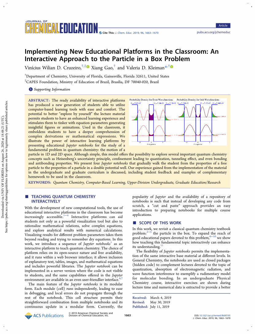
Figure 1. Wave functions and probability densities for (a) free particle and fully defined momentum, (b) free particle with an equally distributedmomentum uncertainty, and (c) free particle with a Gaussian distributed momentum uncertainty.

Journal of Chemical Education Article

DOI: 10.1021/acs.jchemed.9b00195J. Chem. Educ. 2019, 96, 1663−1670

1664

http://pubs.acs.org/doi/suppl/10.1021/acs.jchemed.9b00195/suppl_file/ed9b00195_si_001.pdf

http://pubs.acs.org/doi/suppl/10.1021/acs.jchemed.9b00195/suppl_file/ed9b00195_si_009.zip

http://kleimanteach.chem.ufl.edu:4000



problems where students use the interactive features of thenotebooks to construct their answer. Implementation of theinteractive Jupyter notebooks in three different courses ispresented in the last section. The notebook material allows thestudents to interactively generate independent graphs for wavefunctions, probability densities, and energy levels for differentvalues of box sizes, particle mass, and potential wells, alongwith explanatory text. Additional details on the calculations,derivations, and graphics are also presented under theSupporting Information (SI).

■ THE NOTEBOOKS

Notebook 1: Free Particle

The first notebook, Free Particle, depicts a particle under a nullpotential. To introduce operators and wave functions proper-ties, the notebook exemplifies how the solution wave function,ψ =

πx( ) ek

ikx12

, which is found as an eigenfunction of the

momentum operator P = −iℏ∂/∂x (Pψk(x) = pψk(x) where p =ℏk), is also an eigenfunction of the Hamiltonian for the freeparticle, where V(x) = 0. This example is based on the use ofcommutator properties of quantum mechanical operators.The notebook provides access to the graphical representa-

tion of wave functions where the momentum parameters canbe easily varied. Figure 1a shows the real and imaginarycomponents of the wave function and its probability density.The student can observe that the probability density is thesame for every value of x and conclude that when the particlehas a well-defined momentum (p = ℏk), the probability offinding the particle is the same everywhere in this one-dimensional space. Using the notebook in class, studentsintroduce different values of the wavenumber k and the lengthx and recalculate these graphs.The concept of localization of a particle is introduced in the

notebook by considering not just a single value of momentum,but a range of momenta. For example, it shows thesuperposition of waves with a range of momenta given by p

= p0 ± Δp. Given that the momentum varies continuously, anintegration is required to perform the superposition of waves.Two cases are presented. In the first case, each wavecontributes equally to the overall superposition:

∫ψ = = ΔΔ −Δ

+Δx N k

N kxx

( ) e d2 sin( )

ek k k

k kikx ik x

0

00

(1)

In the latter example, the distribution of momenta ismodulated with a Gaussian function

∫ψ

π

=

= Δ

Δ −∞

+∞− − Δ

− Δ

x N k

N k

( ) e e d

2 e e

kk k k ikx

x k ik x

( ) /2

1/2

02 2

2 20 (2)

where N is a normalization constant.Figure 1b shows the first wave function and its probability

density. When k0 > Δk, the cos(k0x) and sin(k0x) componentsoscillate with a higher frequency (k0) and are modulated by asinusoidal component with lower frequency (Δk). The studentcan test it with different parameters to generate plots where theprobability density to find the particle is shown localizedaround x = 0. If Δk is very small, the particle will still bedelocalized; as Δk increases, the particle becomes morelocalized in a specific region around x = 0. The observedincremental localization is used to introduce the concept ofuncertainty, and how as the uncertainty in the momentumincreases (larger Δk) the uncertainty in the position decreases,with the particle becoming more localized. This behavior ispredicted by Heisenberg’s uncertainty principle. The inter-active graphical representation, with the possibility of varyingΔk, allows students to grasp the concept and to understand themeaning of an equation seen in General Chemistry, whichcontinues to puzzle even some advanced chemistry students.The second example of superposition of waves (Figure 1c) is

constructed such that each k-wave is modulated by a Gaussiandistribution with the maximum contribution from k0 andsmaller contributions from waves with other k values. Once

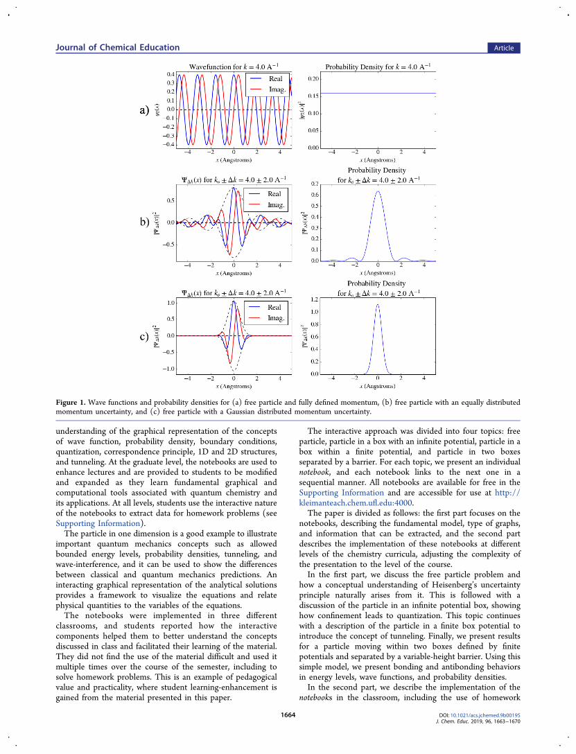
Figure 2. Energy level diagram for an electron inside a square 2D box of dimensions 5 Å × 5 Å. The energy degeneracy is observed, for example, forthe states corresponding to (n, m) = (3, 2) and (2, 3) which have the same energy (19.555 eV). Their corresponding wave functions are plotted inthe right side, showing a different distribution of nodes for each state described by a different wave function.



1665



again, the probability density is localized around x = 0,showing that a decreasing value of Δk could yield a moreprecise value for the momentum, though still leading todelocalization in the position of the particle, as the reader isencouraged to check.

Notebook 2: Particle in a Box with Infinite Potential Walls

The next notebook presents the constrained motion of aparticle, allowing it to move freely only within a certain regionof a 1D space. The concept of Boundary Conditions (ψn(0) =ψn(L) = 0) is introduced, and the normalized wave functionsand allowed energy values are presented. Students areintroduced to quantization by highlighting the differencebetween the free particle results shown in notebook 1 andthose in notebook 2, where not every energy value is allowed.The energies depend on the quantum number n, which is adirect consequence of the boundary conditions. Students aretaught how the confinement of the particle between x = 0 andx = L leads to quantization of its energy.By making use of the interactive platform, the instructor can

present several insightful graphs. These graphs clearly depictthe spacing between energy levels (increasing linearly withincreasing n), a dependency that is highlighted in class andutilized in homework problems (Supporting Information). Thegraphical representation is used to introduce the nodes of awave function and to count them for different values of n toestablish the “n − 1 rule”. The interactive plotting of this figurefor different parameters is used to show how the characteristicsof the wave functions (boundary condition, shape, number ofmaxima, minima, and nodes) remain the same for a givenquantum number. The provided notebook encourages thestudent to compare the characteristics of wave functions,probability densities, and energy levels for boxes of differentsize and particles of different mass.Notebook 2 also includes a brief discussion of a particle in a

two-dimensional box. The introduction of a second dimension(and therefore a second quantum number) opens thepossibility of different states with the same energy and allowsthe teacher to introduce the concept of degeneracy and itsexistence in multidimensional systems. The difference betweenan energy level and a state is examined with the help of a heatplot for the wave functions and an energy diagram. Figure 2shows how the state described by the wave function ψ3,2(x, y)has a different spatial distribution than the state described bythe wave function ψ2,3(x, y), even though the energy levels for

n, m = 2, 3 and for n, m = 3, 2 have the same energy. Studentscan graphically generate the wave function for differentcombinations of quantum numbers (n, m) and evaluatedegeneracy as observed in Figure 2. More details are presentedin the Supporting Information where a homework example isalso presented.

Notebook 3: Particle in a Box with Finite Potential Walls

In order to understand the effect of the height of the box wall,notebook 3 considers a particle moving freely within the wallsof a box defined by f inite potentials. The box has length L, andVo is the depth of its potential. In this notebook we choose tomove the center of the box to x = 0 yielding a symmetricpotential V(−x) = V(x). This is an important point to call tothe attention of students, since a common mistake ofundergraduate students is to assume absolute properties forthe position of the box. As students interacted with thesenotebooks in the classroom, we observed that, by plotting thewave function or probability density for boxes centered atdifferent values of x, students better captured the relativenature of the axes of motion.The notebook describes the Schro dinger equation in the

different regions and finds a general solution for the regioninside the box, ψ(x) = q1 cos(kx) + q2 sin(kx), and for theregion outside the box, ψ(x) = q1e

αox + q2e−αox, where q1 and q2

are coefficients defined by the boundary conditions and

α = >−ℏ

0m V Eo2 2 ( )o

2 .

The classroom presentation of this notebook emphasizes thePostulates of Quantum Mechanics, indicating that the wavefunction must remain finite as x → ±∞, leading to q1 = 0 if x→ +∞ and q2 = 0 if x → −∞. The finite-wave functionpostulate defines the constraints for a unique set of solutions.The notebook highlights the importance of BoundaryConditions and how they must be obeyed to fully describe aspecific system: the wave function must have the same value atx = ±L/2 whether this position is reached from the outside orfrom the inside of the box.For even potentials there are two families of solutions with

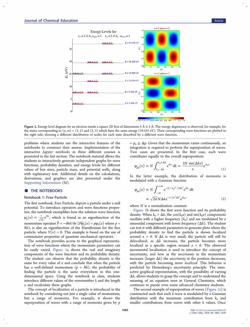
ψ(−x) = ψ(x) or ψ(−x) = −ψ(x) (details in SupportingInformation). In both cases, the boundary conditions imposeconstraints on the αo parameter, associated with the energy.As the notebook shows, it is not possible to obtain an

analytical expression for the unknown values of E. Whenanalytical solutions cannot be found, graphical or numerical

Figure 3. Allowed values of E found graphically for a particle in a finite box with Vo = 8 eV and L = 10 Å. The points of intersection of the twocurves correspond to the E values for bound states. The reader may go to the Jupyter notebook to generate this figure for other values of Vo and L.



1666






methods are commonly used, and this notebook exemplifiesone such case (Figure 3). It provides a simple example to teachadvance undergraduate and graduate students the techniquesfor finding nonanalytical solutions. Students learn by visual-ization that the lowest allowed energy corresponds to an evensolution.Although possible, it is hard to read a precise numerical

value from a plot; thus, the interactive platform is used tonumerically find the (more) accurate allowed values of E. TheJupyter notebook provides the answers and creates a figureshowing all the states with energies lower than the wallpotential Vo; thus, the student can see the number of boundstates, their energies, and the energy spacing between them.

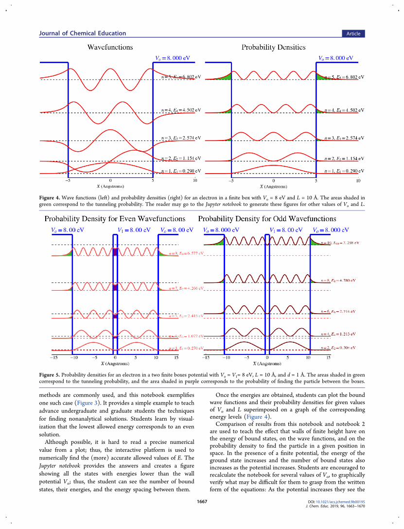
Once the energies are obtained, students can plot the boundwave functions and their probability densities for given valuesof Vo and L superimposed on a graph of the correspondingenergy levels (Figure 4).Comparison of results from this notebook and notebook 2

are used to teach the effect that walls of finite height have onthe energy of bound states, on the wave functions, and on theprobability density to find the particle in a given position inspace. In the presence of a finite potential, the energy of theground state increases and the number of bound states alsoincreases as the potential increases. Students are encouraged torecalculate the notebook for several values of Vo, to graphicallyverify what may be difficult for them to grasp from the writtenform of the equations: As the potential increases they see the

Figure 4. Wave functions (left) and probability densities (right) for an electron in a finite box with Vo = 8 eV and L = 10 Å. The areas shaded ingreen correspond to the tunneling probability. The reader may go to the Jupyter notebook to generate these figures for other values of Vo and L.

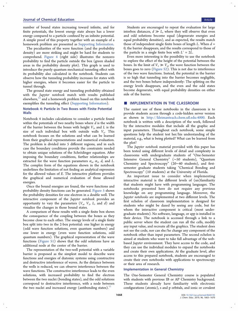
Figure 5. Probability densities for an electron in a two finite boxes potential with Vo = V1= 8 eV, L = 10 Å, and d = 1 Å. The areas shaded in greencorrespond to the tunneling probability, and the area shaded in purple corresponds to the probability of finding the particle between the boxes.



1667


number of bound states increasing toward infinite, and forfinite potentials, the lowest energy state always has a lowerenergy compared to a particle confined by an infinite potential.A simple proof of this property together with an example of ahomework problem are presented as Supporting Information.The peculiarities of the wave function (and the probability

density) are more striking and might be hard for students tocomprehend. Figure 4 (right side) illustrates the nonzeroprobability to find the particle outside the box (green shadedareas in the probability density plot). This graph is used tointroduce the purely quantum mechanical tunneling effect withits probability also calculated in the notebook. Students canobserve how the tunneling probability increases for states withhigher energies, where it becomes easier for the particle totunnel through.The ground state energy and tunneling probability obtained

with the Jupyter notebook match with results publishedelsewhere,12 and a homework problem based on this notebookexemplifies the tunneling effect (Supporting Information).

Notebook 4: Particle in Two Boxes with Finite PotentialWalls

Notebook 4 includes calculations to consider a particle foundwithin the potentials of two nearby boxes where d is the widthof the barrier between the boxes with height V1, and L is thesize of each individual box with outside walls Vo. Thisnotebook focuses on the solutions and what can be learnedfrom their graphical representations and numerical evaluation.The problem is divided into 5 different regions, and in eachcase the boundary conditions provide the constraints neededto obtain unique solutions of the Schro dinger equation. Afterimposing the boundary conditions, further relationships areextracted for the wave function parameters αo, α1, d, and L.The complex form of the equations shown in the notebookunderlines the limitation of not finding an analytical expressionfor the allowed values of E. The interactive platform providesthe graphical and numerical evaluation of those allowedenergies.Once the bound energies are found, the wave functions and

probability density functions can be generated. Figure 5 showsthe probability densities for one electron in a double well. Theinteractive component of the Jupyter notebook provides anopportunity to vary the parameters (Vo, V1, L, and d) andvisualize the changes in those bound states.A comparison of these results with a single finite box shows

the consequence of the coupling between the boxes as theybecome close to each other. The energy levels of a single finitebox split into two in the 2-box potential: one higher in energy(odd wave function solutions, even quantum numbers) andone lower in energy (even wave function solutions, oddquantum numbers). The graphical representation of the wavefunctions (Figure S1) shows that the odd solutions have anadditional node at the center of the barrier.The representation of the two-well potential with a variable

barrier is proposed as the simplest model to describe wavefunctions and energies of diatomic systems using constructiveand destructive interference of waves. As the distance betweenthe wells is reduced, we can observe interference between thewave functions. The constructive interference leads to the evensolutions, with increased probability to find the electronbetween the two nuclei (bonding states), and the odd solutionscorrespond to destructive interference, with a node betweenthe two nuclei and increased energy (antibonding states).11

Students are encouraged to repeat the evaluation for largeinterbox distances, d ≫ L, where they will observe that evenand odd solutions become equal (degenerate energies andequal probability densities), and as expected, the results matchthose of independent single finite boxes of length L. When d =0, the barrier disappears, and the results correspond to those ofthe particle in a single finite box with L′ = 2L.Even more interesting is the possibility to use the notebook

to explore the effect of the height of the potential between theboxes. In the limit of V1 ≫ Vo, the wave function between theboxes goes to zero (Figure S2). This is not due to interferenceof the two wave functions. Instead, the potential in the barrieris so high that tunneling into the barrier becomes negligible,and the two boxes behave independently: The splitting on theenergy levels disappears, and the even and the odd statesbecome degenerate, with equal probability densities on eitherside of the barrier.

■ IMPLEMENTATION IN THE CLASSROOM

The easiest use of these notebooks in the classroom is toprovide students access through a code-hidden server versionas shown in http://kleimanteach.chem.ufl.edu:4000. Eachnotebook is written with a description of the work, followedby the interactive modules that include all the graphic andinput parameters. Throughout each notebook, some simplequestions help the student test her/his understanding of thematerial, e.g., what is being plotted? What can be learned fromthe plot?The Jupyter notebook material provided with this paper has

been tested using different levels of detail and complexity inclassrooms with undergraduate students of “One-SemesterIntensive General Chemistry” (∼50 students), “QuantumChemistry and Spectroscopy” (20−40 students), and first-semester graduate students taking “Chemical Bonding andSpectroscopy” (10 students) at the University of Florida.An important issue to consider when implementing

interactive material is the different levels of (un)familiaritythat students might have with programming languages. Thenotebooks presented here do not require any previousknowledge on any programming language. Moreover, theJupyter notebooks are implemented at two different levels. Thefirst echelon of classroom implementation is designed forstudents who might be dazed by seeing any code, but forwhom the interactive component is critical (most under-graduate students). No software, language, or app is installed intheir device. The notebook is accessed through a link to apublic server where the student can run all the cells, modifyany input value, and recreate all the graphics. The student doesnot see the code, nor can she/he change any component of thenotebook other than input parameters. The second echelon isaimed at students who want to take full advantage of the web-based Jupyter environment. They have access to the code, andthey can use the individual modules to expand the notebooksand create their own applications. At the graduate level, afteraccess to this prepared notebook, students are encouraged tocreate their own notebooks with applications to spectroscopyor their area of research.

Implementation in General Chemistry

The One-Semester General Chemistry course is populatedwith students with previous IB or AP Chemistry background.These students already have familiarity with electronicconfigurations (atomic), s and p orbitals, and ionic or covalent



1668







bonds based on electronegativity tables. In most cases, theirskills are based on repetitive problem solving; i.e., studentsmight know that H has a 1s1 electronic configuration but haveno understanding of quantization, what is an orbital, what is aprobability density, degeneracy, etc.For this class, notebook 2 (Particle in an infinite potential

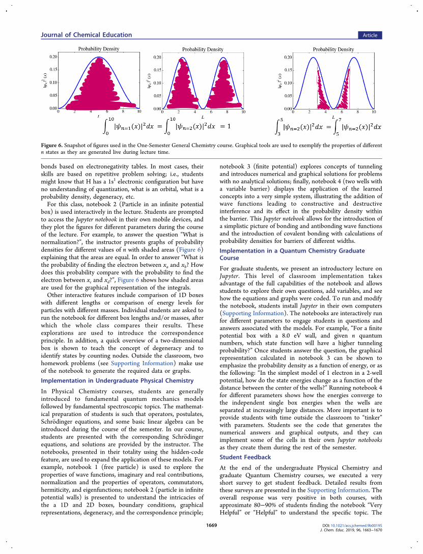
box) is used interactively in the lecture. Students are promptedto access the Jupyter notebook in their own mobile devices, andthey plot the figures for different parameters during the courseof the lecture. For example, to answer the question “What isnormalization?”, the instructor presents graphs of probabilitydensities for different values of n with shaded areas (Figure 6)explaining that the areas are equal. In order to answer “What isthe probability of finding the electron between xa and xb? Howdoes this probability compare with the probability to find theelectron between xc and xd?”, Figure 6 shows how shaded areasare used for the graphical representation of the integrals.Other interactive features include comparison of 1D boxes

with different lengths or comparison of energy levels forparticles with different masses. Individual students are asked torun the notebook for different box lengths and/or masses, afterwhich the whole class compares their results. Theseexplorations are used to introduce the correspondenceprinciple. In addition, a quick overview of a two-dimensionalbox is shown to teach the concept of degeneracy and toidentify states by counting nodes. Outside the classroom, twohomework problems (see Supporting Information) make useof the notebook to generate the required data or graphs.

Implementation in Undergraduate Physical Chemistry

In Physical Chemistry courses, students are generallyintroduced to fundamental quantum mechanics modelsfollowed by fundamental spectroscopic topics. The mathemat-ical preparation of students is such that operators, postulates,Schro dinger equations, and some basic linear algebra can beintroduced during the course of the semester. In our course,students are presented with the corresponding Schro dingerequations, and solutions are provided by the instructor. Thenotebooks, presented in their totality using the hidden-codefeature, are used to expand the application of these models. Forexample, notebook 1 (free particle) is used to explore theproperties of wave functions, imaginary and real contributions,normalization and the properties of operators, commutators,hermiticity, and eigenfunctions; notebook 2 (particle in infinitepotential walls) is presented to understand the intricacies ofthe a 1D and 2D boxes, boundary conditions, graphicalrepresentations, degeneracy, and the correspondence principle;

notebook 3 (finite potential) explores concepts of tunnelingand introduces numerical and graphical solutions for problemswith no analytical solutions; finally, notebook 4 (two wells witha variable barrier) displays the application of the learnedconcepts into a very simple system, illustrating the addition ofwave functions leading to constructive and destructiveinterference and its effect in the probability density withinthe barrier. This Jupyter notebook allows for the introduction ofa simplistic picture of bonding and antibonding wave functionsand the introduction of covalent bonding with calculations ofprobability densities for barriers of different widths.

Implementation in a Quantum Chemistry GraduateCourse

For graduate students, we present an introductory lecture onJupyter. This level of classroom implementation takesadvantage of the full capabilities of the notebook and allowsstudents to explore their own questions, add variables, and seehow the equations and graphs were coded. To run and modifythe notebook, students install Jupyter in their own computers(Supporting Information). The notebooks are interactively runfor different parameters to engage students in questions andanswers associated with the models. For example, “For a finitepotential box with a 8.0 eV wall, and given n quantumnumbers, which state function will have a higher tunnelingprobability?” Once students answer the question, the graphicalrepresentation calculated in notebook 3 can be shown toemphasize the probability density as a function of energy, or asthe following: “In the simplest model of 1 electron in a 2-wellpotential, how do the state energies change as a function of thedistance between the center of the wells?” Running notebook 4for different parameters shows how the energies converge tothe independent single box energies when the wells areseparated at increasingly large distances. More important is toprovide students with time outside the classroom to “tinker”with parameters. Students see the code that generates thenumerical answers and graphical outputs, and they canimplement some of the cells in their own Jupyter notebooksas they create them during the rest of the semester.

Student Feedback

At the end of the undergraduate Physical Chemistry andgraduate Quantum Chemistry courses, we executed a veryshort survey to get student feedback. Detailed results fromthese surveys are presented in the Supporting Information. Theoverall response was very positive in both courses, withapproximate 80−90% of students finding the notebook “VeryHelpful” or “Helpful” to understand the specific topic. The

Figure 6. Snapshot of figures used in the One-Semester General Chemistry course. Graphical tools are used to exemplify the properties of differentn states as they are generated live during lecture time.



1669





graduate level implementation needed more participation fromstudents, and they were required to create their own Jupyternotebook for other topics. For the graduate students, asexpected, the results were tainted by their experiences trying towrite their own notebooks. As a follow-up to this survey wecreated the server version, which removes any visible code andallows them to focus only on the quantum mechanics. This isquite reasonable for an undergraduate level course, although atthe graduate level we will continue to provide the full code ofthe Jupyter notebooks. In today’s academic environment, everygraduate student needs to learn at least a little bit of aprogramming language, and Jupyter has become tremendouslyuseful for physical chemists.In our experience, using this material enabled students to

better understand concepts like plotting and representing wavefunctions and probability densities, localization and delocaliza-tion of wave functions, boundary conditions, tunnelingprobabilities, degeneracy, and difference between even andodd solutions, among others. This conclusion is based on thetype of questions students asked during office hours, thequality of the plots they presented to answer homeworkquestions, and the fact that, during lectures of other topics,students referred back to the plots encountered in thesenotebooks to try to understand the new subjects.For example, during lecture, when the instructor introduced

the harmonic oscillator and its zero point energy in theundergraduate Physical Chemistry course, students referred tothe particle in the box energy diagrams and the energydependence on “n” observed in the second notebook; whenthe instructor talked about bonding and antibonding MOs inH2

+ and introduced a linear combination of atomic orbitals toform an MO, students recalled the two boxes separated by abarrier they had seen at the beginning of the semester andasked whether the LCAO was in any way related to the sum ofwaves they had seen in the last notebook. These types ofquestions and connections between concepts had not beenobserved in previous semesters, where no interactive graphicalplatform had been used.We note that these notebooks are meant to complement a

lecture, not to replace it.

■ CONCLUSIONSIn this work, we showed how the quantum mechanicaldescription of a particle in simple model potentials can beexplored and taught interactively in the classroom with the useof the Jupyter notebook platform. While the concepts are well-developed in standard textbooks, our students reported anenhanced learning experience from the use of this materialwhich allowed them to better grasp the concepts andmathematical equations presented in class.We hope this paper will encourage students and educators to

develop new educational interactive platforms, in the area ofquantum chemistry.

■ ASSOCIATED CONTENT*S Supporting Information

The Supporting Information is available on the ACSPublications website at DOI: 10.1021/acs.jchemed.9b00195.

Homework problems (PDF, DOCX)Student survey information (PDF, DOCX)Proofs and additional plots (PDF, DOCX)Instructions for using Jupyter Notebooks (PDF, DOCX)

Jupyter notebook files (ZIP)

■ AUTHOR INFORMATIONCorresponding Author

*E-mail: [email protected]

Vinícius Wilian D. Cruzeiro: 0000-0002-4739-5447Valeria D. Kleiman: 0000-0002-9975-6558Notes

The authors declare no competing financial interest.

■ ACKNOWLEDGMENTSThis work was supported by the National Science FoundationCHE-1802240. V.W.D.C. acknowledges the financial supportof CAPES (Brazil) through a graduate fellowship.

■ REFERENCES(1) Perez, F.; Granger, B. E. IPython: A System for InteractiveScientific Computing. Comput. Sci. Eng. 2007, 9 (3), 21−29.(2) Cohen-Tannoudji, C.; Diu, B.; Laloe, F. Quantum Mechanics,77th ed.; Wiley-VCH, 1977; Vol. 1.(3) Levine, I. N. Quantum Chemistry, 5th ed.; Prentice-Hall: UpperSaddle River, NJ, 2000.(4) Fayer, M. D. Elements of Quantum Mechanics; Oxford UniversityPress: New York, NY, 2001.(5) Griffiths, D. J. Introduction to Quantum Mechanics, 2nd ed.;Pearson Prentice Hall: Upper Saddle River, NJ, 2005.(6) El-Issa, H. D. The Particle in a Box Revisited. J. Chem. Educ.1986, 63 (9), 761.(7) Tisko, E. L. Visualizing Particle-in-a-Box Wavefunctions UsingMathcad. J. Chem. Educ. 2003, 80 (5), 581.(8) Casaubon, J. I.; Doggett, G. Variational Principle for a Particle ina Box. J. Chem. Educ. 2000, 77 (9), 1221.(9) Volkamer, K.; Lerom, M. W. More about the Particle-in-a-BoxSystem: The Confinement of Matter and the Wave-Particle Dualism.J. Chem. Educ. 1992, 69 (2), 100.(10) Liang, Y. Q.; Zhang, H.; Dardenne, Y. X. MomentumDistributions for a Particle in a Box. J. Chem. Educ. 1995, 72 (2), 148.(11) Cruzeiro, V. W. D.; Roitberg, A.; Polfer, N. C. InteractivelyApplying the Variational Method to the Dihydrogen Molecule:Exploring Bonding and Antibonding. J. Chem. Educ. 2016, 93 (9),1578−1585.(12) Blank, N. C.; Clemons, K.; Crowdis, R.; Estridge, C.; Foster,M.; Gash, S.; Gish, B.; Gollihue, B.; Henzman, C.; Hernandez, D.;et al. Thinking Outside the (Particle in a) Box: Tunneling,Uncertainty and Dimensional. Analysis. Chem. Educ. 2010, 15, 134−140.



1670

http://pubs.acs.org

http://pubs.acs.org

http://pubs.acs.org/doi/abs/10.1021/acs.jchemed.9b00195


http://pubs.acs.org/doi/suppl/10.1021/acs.jchemed.9b00195/suppl_file/ed9b00195_si_002.docx








mailto:[email protected]

http://orcid.org/0000-0002-4739-5447

http://orcid.org/0000-0002-9975-6558


Journal of Chemical Education 4/9/19 Page 1 of 3

Supporting Information for " Implementing new educational platforms in the classroom: an interactive approach to the Particle in a Box problem "

Vinícius Wilian D. Cruzeiro a,b, Xiang Gao a, Valeria D. Kleiman* a

a Department of Chemistry, University of Florida, Gainesville, Florida, 32611, United Statesb CAPES Foundation, Ministry of Education of Brazil, Brasília – DF 70040-020, Brazil

HOMEWORK PROBLEMS ASSOCIATED WITH JUPYTER NOTEBOOKS

One-Semester General Chemistry

1. Exploring a particle in a 2-Dimensional box. Use the link http://kleimanteach.chem.ufl.edu:4000/02_particle_in_an_infinite_potential_box.html to further explore the model of a particle in 1D and in a 2D box. For a particle in a square box. 8.72 Åa. How many degenerate states are possible for Energies below 13 eV? (Hint: use a

value of n or m larger than 4)b. For each energy level that has degenerate states, list all the groups of degenerate

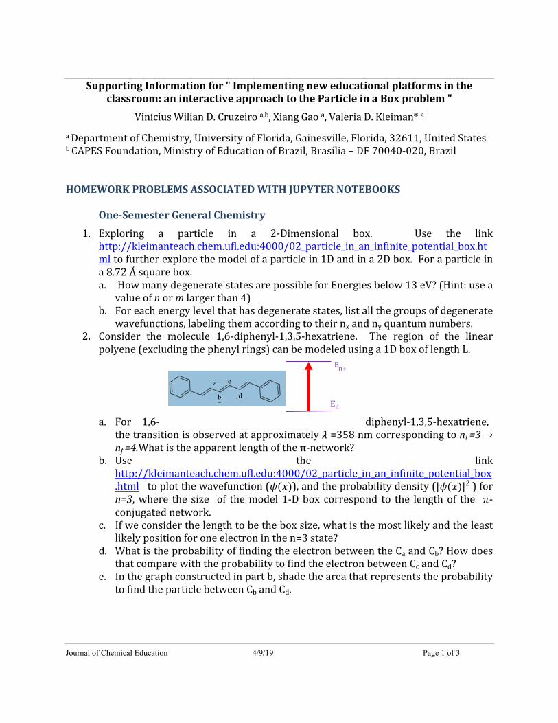
wavefunctions, labeling them according to their nx and ny quantum numbers. 2. Consider the molecule 1,6-diphenyl-1,3,5-hexatriene. The region of the linear

polyene (excluding the phenyl rings) can be modeled using a 1D box of length L.

a. For 1,6- diphenyl-1,3,5-hexatriene, the transition is observed at approximately =358 nm corresponding to ni =3 → 𝜆nf =4.What is the apparent length of the π-network?

b. Use the link http://kleimanteach.chem.ufl.edu:4000/02_particle_in_an_infinite_potential_box.html to plot the wavefunction ( ), and the probability density ( ) for 𝜓(𝑥) |𝜓(𝑥)|2 n=3, where the size of the model 1-D box correspond to the length of the -𝜋conjugated network.

c. If we consider the length to be the box size, what is the most likely and the least likely position for one electron in the n=3 state?

d. What is the probability of finding the electron between the Ca and Cb? How does that compare with the probability to find the electron between Cc and Cd?

e. In the graph constructed in part b, shade the area that represents the probability to find the particle between Cb and Cd.

En+1

En

http://kleimanteach.chem.ufl.edu:4000/02_particle_in_an_infinite_potential_box.html





Undergraduate Physical Chemistry

The following problems are solved using the Jupyter notebooks introduced in class to obtain the required data,

1. Use the Jupyter notebook to evaluate the energy levels of 1 electron in a box 1 Angstrom wide.

a. Use those values to construct a graph with 4 plots:i. Plot the energy of each level as a function of quantum number.

ii. Plot the energy separation between levels as a function of quantum number.

iii. Plot together these two quantities.iv. Plot the ratio of ΔE/E.

b. What can you conclude about the behavior of the system as the quantum number increases (at a fix and given T)? (Hint: Bohr's correspondence principle)

This problem can also be tried using H2 molecules, m(H2) = 2x1836me, in a 1D box of length 500 pm.

2. Show that the function

is an eigenfunction of the nx ,nyx, y Asin nx

ax

sinnyb

y

Hamiltonian of a particle in a 2D box of lengths a x b. a. Given a 5 Å x 5 Å square box, are there any degenerate states at or below

E=19.6 eV? If so, write the complete eigenfunction for each state (assume mass =mass of 1 electron, which is what the notebooks uses).

b. Sketch the the plot for the probability density for each state found in part a. and compare it to the graphs obtained from the notebook.

c. How many nodes are there in each direction? Can you predict the number of nodes without performing the plot of the 2D wavefunction?

3. Let's look at the behavior of particles confined within finite-size potentials.a. What is the major difference in the Probability Densities for a particle

constrained within a box of infinite-height potentials versus a particle confined in a finite-height potential?

b. Consider a particle within a potential box of 1 nm and confined within a V=15 eV potential. What is the state with largest tunneling probability? What is the probability of tunneling outside the classically allowed region?

4. Consider a particle in a 2-well of V0=6 eV, L= 5 Å and barrier V1=8 eV. For n =3, plot the Probability density of finding the particle in the classically forbidden region as a function of distance between the wells (work with distance between 0 and 5 Å. If you are looking for the maximum probability to find the particle within the barrier, what would be the optimal distance between wells?


Graduate Level Chemical BondingAfter students had access to the Jupyter notebooks, they are required to build their own notebooks. For this assignment, students may modify the notebooks provided and create their own components.

1. A rough treatment of -electrons in a conjugated molecule regards these electrons 𝜋as particles moving in a “particle in the box potential”, where the length of the box is somewhat longer than the conjugated chain. The Pauli exclusion principle allows no more than 2 electrons in each energy level. For butadiene CH2=CHCH=CH2, taking the box to be 7.0 Å, estimate the of the light absorbed when a -electron is excited 𝜆 𝜋from the highest occupied level to the lowest unoccupied level. Compare the results with the experimental value of = 217 nm and draw some conclusions on the limitations of the model.

2. Consider a square box of length 1 Å x 1 Å . Use Jupyter Notebooks to:a. Draw the contour plot for the wavefunction and the probability density of an

electron in a 2D box with ( , )= (1,2) and (2,1). xn ynb. In a graph, show that for a constant value of , the functions look like a 1-D x

particle in a box with nodes.1yn c. Write a short script to evaluate the probability of finding the particle in the

region between (0.2, 0.7) and (0.2 + x, 0.7 + y) Å.d. Compare that probability with the probability of finding the particle in the

region between (0.8, 0.3) and (0.8 - x, 0.3 - y) Å. For this comparison, a graphical representation is good: Plot the Probability Density as a function of position and use shaded areas to show the integrated values.

3. Consider the simplistic description of H2+ as a 1D box of length 95 pm. Use Jupyter

Notebooks to evaluate the energies of the eigenstates of a particle within that box.a. Graph 3 plots: in the first one, plot the Energy of each level as a function of

quantum number; on the second one: plot the Energy separation between levels as a function of quantum number, and on the last one, plot the ratio of ΔE/E.

b. Compare these plots with kT (for a given T), what can you say about the behavior of the molecule as the quantum number increases? (Hint: Bohr's correspondence principle)





STUDENT SURVEYSome responses from survey of students who used the Jupyter notebooks.

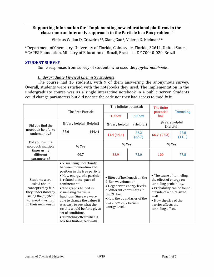
Undergraduate Physical Chemistry studentsThe course had 16 students, with 9 of them answering the anonymous survey.

Overall, students were satisfied with the notebooks they used. The implementation in the undergraduate course was as a single interactive notebook in a public server. Students could change parameters but did not see the code nor they had access to modify it.

The infinite potential:The Free Particle

1D box 2D box

The finite potential

boxTunneling

% Very helpful (Helpful) % Very helpful(Helpful)Did you find the

notebook helpful to understand...?

% Very helpful (Helpful)

55.6 (44.4)44.4 (44.4) 22.2

(66.7) 66.7 (22.2) 77.8 (11.1)

% Yes % Yes Did you run the notebook multiple

times using different

parameters?

% Yes

66.7 88.9 75.0 100 77.8

Students were asked about

concepts they felt they understood by

using the Jupyter notebooks, written in their own words

Visualizing uncertainty between momentum and position in the free particle How energy, of a particle, is related to its space of confinement The graphs helped in visualizing the wave functions. Since we were able to change the values it was easy to see what the results would be for a given set of conditions. Tunneling effect when a box has finite-sized walls

Effect of box length on the 2-Box wavefunction Degenerate energy levels of different coordinates in the 2D boxHow the boundaries of the box allow only certain energy levels

The cause of tunneling, the effect of energy on tunneling probability, Probability can be found outside of a finite-sized wall How the size of the barrier affects the tunneling effect.


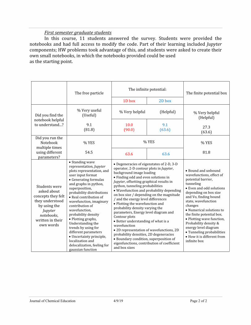
First semester graduate studentsIn this course, 11 students answered the survey. Students were provided the

notebooks and had full access to modify the code. Part of their learning included Jupyter components; HW problems took advantage of this, and students were asked to create their own small notebooks, in which the notebooks provided could be used as the starting point.

The infinite potential:The free particle

1D box 2D box

The finite potential box

% Very helpful (Helpful)Did you find the

notebook helpful to understand...?

% Very useful (Useful)

9.1 (81.8)

10.0 (90.0)

9.1 (63.6)

% Very helpful (Helpful)

27.3 (63.6)

% YESDid you run the

Notebook multiple times using different

parameters?

% YES

54.5 63.6 63.6

% YES

81.8

Students were asked about

concepts they felt they understood

by using the Jupyter

notebooks, written in their

own words

Standing wave representation, Jupyter plots representation, and user input format Generating formulas and graphs in python, superposition, probability distributions Real contribution of wavefunction, imaginary contribution of wavefunction, probability density Plotting graphs, Understanding the trends by using for different parameters Uncertainty principle, localization and delocalization, feeling for gaussian function

Degeneracies of eigenstates of 2-D, 3-D operator, 2-D contour plots in Jupyter, background image loading Finding odd and even solutions in Jupyter, offsetting graphical results in python, tunneling probabilities Wavefunction and probability depending on box size / depending on the magnitude / and the energy level differences Plotting the wavefunction and probability density varying the parameters, Energy level diagram and Contour plots Better understanding of what is a wavefunction 2D representation of wavefunctions, 2D probability densities, 2D degeneracies Boundary condition, superposition of eigenfunctions, contribution of coefficient and box sizes

Bound and unbound wavefunctions, effect of potential barrier, tunneling Even and odd solutions depending on box size and Vo, finding bound state, wavefunction changes Numerical solutions to the finite potential box. Plotting wave function, Probability density & energy level diagram Tunneling probabilities How it is different from infinite box





PROOF: WAVEFUNCTIONS CAN BE EVEN OR ODD WHEN THE POTENTIAL IS EVEN

For even potentials there are two families of solutions with : or x x

. Here we show the proof. Let’s assume the potential is even, that is, x x

that . The time-independent Schrödinger equation is: V x V x

(1)

22

22d x

V x x E xm dx

h

We can now write the equation for :x x

(2)

22

22d x

V x x E xm dx

h

As , we see that and obey exactly the same equation. V x V x x x

For this reason, and must be equivalent solutions except for a x x multiplicative constant, that is:

(3) x a x

Because and must have the same norm, we have that . This x x 1a leads then to two possibilities: (even wavefunction) and (odd 1a 1a wavefunction).

It is important to mention that it is possible to make linear combinations of and in such a way that it would still be a solution but with undefined x x

parities.


PROOF: WHY THE ENERGY LEVELS SHIFT DOWN FOR THE FINETE BOX

Let’s consider the following potential:

(4) 2

0 for - 2 2,for other valueso o

L LxV x

V V V

We see that for we have a particle in a finite box potential with a potential 0

depth equal to , and for the potential depth is equal to . Let’s assume that oV 1 2V, therefore increases with . We have that: 2 oV V ,V x

(12) 2

0 for -, 2 2for other valueso

L LxV x

V V

Therefore, as , we have .2 oV V ,0

V x

According to the Hellmann-Feynman theorem, we have that:

(13), *, ,

ˆn

n n

dE dH dxd d

As the kinetic energy operator does not depend on , we have that:

(14) , *, ,

,0n

n n

dE V xdx

d

Therefore, as , the higher the value of , the higher the value of the , 0ndE

d

energy level is (or the energy value remains the same if ). So we can , 0ndEd

conclude: . This conclusion is still true on the limit in which 2 for for n n oE V E V

, and explains why the energy levels for the finite box shift down in 2V comparison to the infinite box levels.


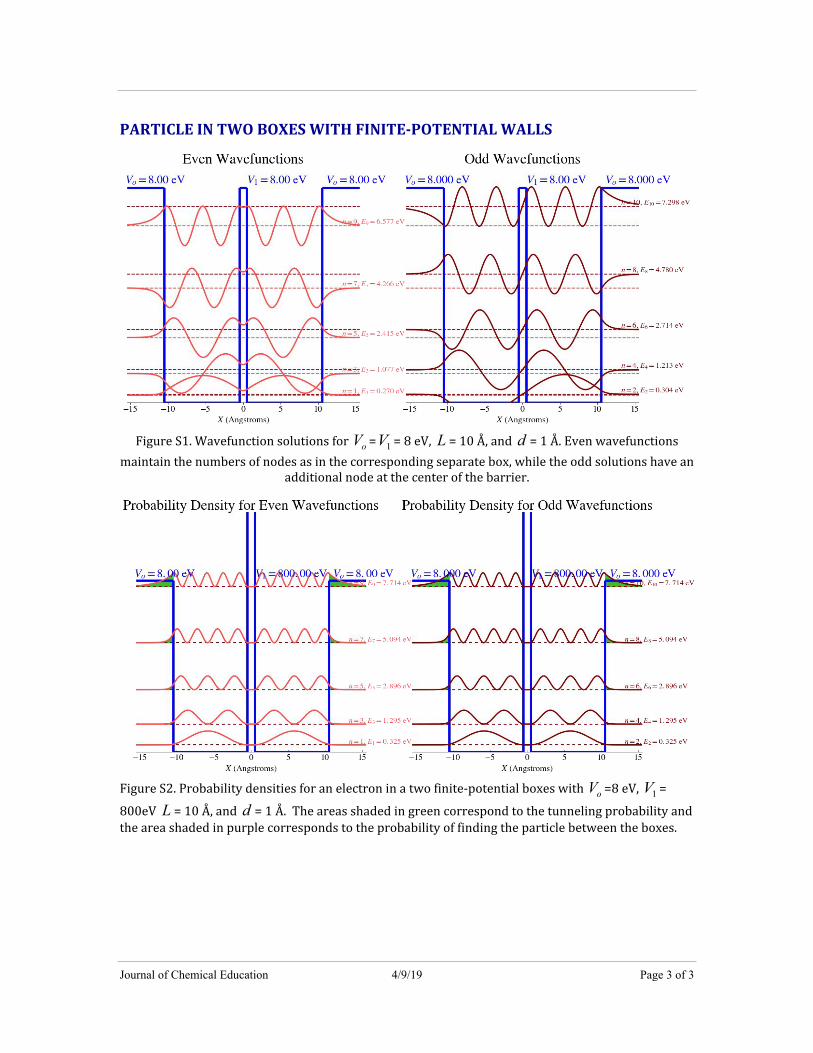
PARTICLE IN TWO BOXES WITH FINITE-POTENTIAL WALLS

Figure S1. Wavefunction solutions for = = 8 eV, = 10 Å, and = 1 Å. Even wavefunctions oV 1V L dmaintain the numbers of nodes as in the corresponding separate box, while the odd solutions have an

additional node at the center of the barrier.

Figure S2. Probability densities for an electron in a two finite-potential boxes with =8 eV, = oV 1V800eV = 10 Å, and = 1 Å. The areas shaded in green correspond to the tunneling probability and L dthe area shaded in purple corresponds to the probability of finding the particle between the boxes.





INSTRUCTIONS FOR RUNNING THE NOTEBOOKS IN A WEB SERVER

To make it convenient for instructors to use the notebook without having to ask students to install and learn the Jupyter environment, we converted the notebook into a webpage where the student could use the notebook with full functionality purely inside a browser. The webpage is hosted at http://kleimanteach.chem.ufl.edu:4000/. Students only need to type numbers into the form and click “Show” button to see the result.The webpage has a server-client architecture where the inputs of students are sent to a server, the server draws the figures and return it back to students to display in the browser. The source code for the server is hosted on GitHub at: https://github.com/zasdfgbnm/a_quantum_particle_moving_in_space-serverInstructors could modify the code on their own and build their own server. The server runs inside Docker, which makes building the server as simple as a single command:“docker build”.

INSTRUCTIONS FOR INSTALLING AND RUNNING JUPYTER NOTEBOOK AND ALL THE NECESSARY LIBRARIES

The host website for Jupyter can be found here: https://jupyter.org/

There are several ways of installing Jupyter notebook (like through pre-packaged distributions as Anaconda, available for several operational systems: https://www.anaconda.com/distribution). Hereafter, we provide step-by-step instructions on how to install Jupyter notebook and all necessary libraries on Windows, Linux and Mac OS.Installation instructions for Windows

1) Download the latest version of Anaconda for Python 3 from: https://www.anaconda.com/distribution/. You will get a *.exe file.

http://kleimanteach.chem.ufl.edu:4000/

https://github.com/zasdfgbnm/a_quantum_particle_moving_in_space-server

http://ipython.org/


2) Install the *.exe file following its instructions. After installation, you should see a new application called “Anaconda Navigator” added to your start menu.

3) Extract the supporting information ZIP file downloaded from the J. Chem. Educ. website and copy its content (Jupyter notebook files in format *.ipynb, and figures in format *.png) somewhere in your home directory, for example, C:\Users\YourUserName . Avoid directories that contain special characters if you run into problems.

4) Open “Anaconda Navigator”, and open “Notebook” from Anaconda Navigator. A browser window should be opened automatically.

5) Navigate to the directory where you put these *.ipynb files, and open the file you want.

Installation instructions for Linux

The following instructions were tested on an Ubuntu machine.1) Download the latest version of Anaconda for Python 3 from:

https://www.anaconda.com/distribution/. You will get a *.sh file.2) Open a terminal window.3) From the same folder where the *.sh file is, execute the following command:

$ bash Anaconda3-*.sh4) Follow the on-screen prompts to complete your installation. When asked

about the initialization of Anaconda in your $HOME/.bashrc file, enter: yes. Once the installation is complete, execute:

$ source ~/.bashrc5) Extract the supporting information ZIP file downloaded from the J. Chem.

Educ. website and copy its content (Jupyter notebook files in format *.ipynb, and figures in format *.png) into the same directory of your terminal window.

6) In your terminal window execute Jupyter notebook with the following command:

$ jupyter notebook7) A tab should open in your web browser. Among the files and subfolders

listed, click on any *.ipynb file to launch that given Jupyter notebook, which will open in a new tab in the browser.

Installation instructions for Mac OSAlthough Python is a default package in Mac OS, we are going to perform a new

installation based on Anaconda to make sure that all the libraries necessary to run all the Jupyter notebook programs provided in this paper are going to run properly.

1) Download the latest version of the Anaconda installation file for Mac OS (*.pkg) from https://www.anaconda.com/distribution. Make sure you download the Python 3 version of anaconda.

https://www.anaconda.com/distribution


2) Execute the *.pkg file by double clicking on it and follow all instructions on the screen.

3) Open a terminal window.4) Extract the supporting information ZIP file downloaded from the J. Chem.

Educ. website and copy its content (Jupyter notebook files in format *.ipynb, and figures in format *.png) into the same directory of your terminal window.

5) In the terminal execute Jupyter notebook with the following command:$ jupyter notebook

6) A tab should open in your web browser. Among the files and subfolders listed, click on any *.ipynb file to launch that given Jupyter notebook, which will open in a new tab in the browser.

How to run the Jupyter notebook programIf the reader is getting started with Jupyter notebooks, introductory lectures written by J. R. Johansson are an excellent starting point and are available at: https://github.com/jrjohansson/scientific-python-lectures . Information about Jupyter notebook can also be gathered from Jupyter’s website: https://jupyter-notebook.readthedocs.io/en/stable/

A Jupyter notebook is structured as a sequence of cells. Roughly speaking, there are two main types of cells: code cells (that contain Python code) and markdown cells (to display text, including in LaTeX format). Our Jupyter notebook programs were written in such a way that the code cells have to be executed in consecutive order. Each code cell can be individually executed by pressing Shift+Enter with the cell selected. A useful way to speed up executing cells in the correct order is to select the cell of interest and then click on “Run All Above” at the tab “Cell” at the toolbar on the upper part of the page.

NOTE: there are some code cell that require the user to enter information before executing. The desired information can be entered in the boxes that appears on the screen right after the cell.

NOTE: A message saying that the notebook has been converted from an older format (v3) to a new format (v4) may appear on the screen when the Jupyter notebook files are open. This is not an issue. The programs will execute normally. The notebook files were written in an older version because newer versions are able to read it, however if the files were written in a newer version users using older versions may not able to open the files.

https://github.com/jrjohansson/scientific-python-lectures

implementing new educational platforms in the classroom

Documents