implementation of a bayesian algorithm into mantid for the

UNIVERSITAT POLITÈCNICA DE CATALUNYA

BACHELOR’S THESIS IN ENGINEERING PHYSICS

Implementation of a Bayesian algorithminto Mantid for the analysis of neutron

scattering data to reveal molecularmovements

Author:Diego Monserrat López

Supervisor:Dr. Luis Carlos Pardo Soto

Group of Characterization of Materials

Barcelona

January 2016

Abstract

Data fitting and model selection lie at the very heart of the scientific method, how-ever, these tasks are often tackled via the use of popular (and typically unquestioned)optimization algorithms of limited validity or flexibility. To circumvent these limita-tions, this work introduces an adaptive Markov chain Monte Carlo method for, throughBayesian Inference, performing fitting of experimental data. This method allows to ob-tain χ2 probability density functions without assuming any frequentist supposition,and taking into account correlation between fitting parameters by direct exploration ofthe parameter space.

This work mainly consists in the creation of a powerful fitting tool based on the afore-mentioned robust inference method. In fact, it is presented the implementation of thealgorithm FABADA (Fitting Algorithm for Bayesian Analysis of Data) within the Man-tid framework. The power of this algorithm is illustrated by revisiting an overarchingand recurring question in the interpretation of quasielastic neutron scattering measure-ments, that is, how many spectral components may (or may not) be justified by theavailable experimental data.

Finally, an accurate Bayesian analysis is performed over real quasielastic neutron scat-tering measurements, in order to study the molecular reorientation dynamics of Cl-adamantane in its plastic phase. A calorimetric study [1] over this compound showsan anomalous heat-capacity behavior around T = 310 K, which is inside the tempera-ture range of the plastically crystalline phase. So, this works has the aim of prove ifthe molecular dynamics can be related with this phenomenon. The analysis performedshows how, since the consideration of Cl-adamantane such as an oblong shaped mole-cule, there is variation on the degree of anisotropy of the rotational diffusion approxi-mately at the temperature of interest.

iii

Acknowledgements

First of all, I would like to express my gratitude to Dr. Luis Carlos Pardo, for givingme the opportunity to work with this project and for his dedication and guidance assupervisor of this bachelor’s thesis. Secondly, I would like to thank the ISIS Molecu-lar Spectroscopy Group, particularly Dr. Félix Fernández-Alonso and Dr. SanghamitraMukhopadhyay, for the great treatment and good advice all they gave me during mystays with the group. I am also grateful to my colleagues Roman Tolchenov, from theMantid Development team, for his valuable guidance with the software development,and Alessandro Vispa, from the Group of Characterization of Materials, for his helpfulcontribution.

Finally, I would like to thank my family and friends, whose support has been invalu-able throughout all these years at university.

v

Contents

Abstract iii

Acknowledgements v

1 Introduction 1

2 Bayesian inference 32.1 The ubiquitous χ2 . . . . . . . . . . . . . . . . . . . . . . . . . . . . . . . . 32.2 Adaptive Markov chain Monte Carlo method . . . . . . . . . . . . . . . . 42.3 FABADA . . . . . . . . . . . . . . . . . . . . . . . . . . . . . . . . . . . . . 62.4 Model selection . . . . . . . . . . . . . . . . . . . . . . . . . . . . . . . . . 7

3 Mantid Implementation 113.1 Using FABADA within Mantid . . . . . . . . . . . . . . . . . . . . . . . . 12

3.1.1 The visual interfaces . . . . . . . . . . . . . . . . . . . . . . . . . . 123.1.2 A look to the results . . . . . . . . . . . . . . . . . . . . . . . . . . 143.1.3 Writing a Python script . . . . . . . . . . . . . . . . . . . . . . . . 17

3.2 Coclusions and prospects . . . . . . . . . . . . . . . . . . . . . . . . . . . 18

4 How many lines are there? 214.1 Data generation . . . . . . . . . . . . . . . . . . . . . . . . . . . . . . . . . 214.2 Model selection . . . . . . . . . . . . . . . . . . . . . . . . . . . . . . . . . 234.3 Conclusions . . . . . . . . . . . . . . . . . . . . . . . . . . . . . . . . . . . 24

5 Neutron scattering overview 255.1 Coherent and incoherent scattering . . . . . . . . . . . . . . . . . . . . . . 255.2 Correlation functions . . . . . . . . . . . . . . . . . . . . . . . . . . . . . . 275.3 IRIS instrument . . . . . . . . . . . . . . . . . . . . . . . . . . . . . . . . . 28

5.3.1 Principle of operation . . . . . . . . . . . . . . . . . . . . . . . . . 29

6 The dynamics of Cl-Adamantane 316.1 Chloroadamantane . . . . . . . . . . . . . . . . . . . . . . . . . . . . . . . 316.2 The QENS experiment . . . . . . . . . . . . . . . . . . . . . . . . . . . . . 326.3 Analysis and discussion . . . . . . . . . . . . . . . . . . . . . . . . . . . . 336.4 Conclusions . . . . . . . . . . . . . . . . . . . . . . . . . . . . . . . . . . . 40

Bibliography 41

vii

Chapter 1

Introduction

Data fitting is the standard way to ascertain how correctly a model describes experi-mental results and to obtain parameters that describe the underlying physics processes.It also allows to perform model selection by quantifying the success of a hypothesis todescribe the experimental measurements. Despite being a crucial component of thescientific method, data fitting is not always tackled via the most appropriate way.

Frequentist methods, such as Levenberg-Marquardt algorithm (also known as thedamped least-squared method), are the most popular when performing data fitting.These methods are based in the minimization of a cost function, usually χ2 (defined insection 2.1). The goal is to obtain the set of parameters’ values, with their associatederrors, which best describes the experimental data (Pi ± εi). Therefore, the minimumvalue for χ2, the associated to optimal values of the parameters, is used as figure ofmerit in order to quantify the fitting quality. In order words, the veracity of the hy-pothesis, which in this case is the mathematical model.

Frequentist approximation for data analysis has as the main drawback that it usu-ally gets stuck in local minima of the χ2 hypersurface when starting far away the globalminimum or if the model is complex. In fact, frequentist methods involve certain sup-positions that deserve to be considered. They suppose that there is only one minimumin the χ2Pi hypersurface and that the functional dependence of χ2Pi is quadraticon each parameter i, therefore only symmetric errors are allowed. Moreover, frequen-tist approach discards possible correlations between parameters.

In front of frequentist approximation we can find Bayesian inference, which doesnot need any supposition on the χ2Pi landscape [2]. A Bayesian analysis resultsin a different completely manner to express fitted parameters and the figure of meritshowing all the complexity of the final solution: they become Probability DistributionFunction (PDFs) obtained directly from exploring the χ2Pi hypersurface. Chapter 2will focus on Bayesian inference as well as on a Markov chain Monte Carlo (MCMC)method, which is a way to achieve the desired PDFs. We also will introduce how toget this technique adaptive in order to optimize the parameter space exploration. Fur-thermore, we will see how Bayesian inference allows to perform model selection in acompletely different way, full of benefits [3].

The main objective of the present thesis is, beyond explaining the intrinsic aspectsof Bayesian analysis as well as showing its advantages with respect to frequentist meth-ods, to convert it into a useful and powerful tool for the user. Therefore, the algorithmFABADA (Fitting Algorithm for Bayesian Analysis of Data) [4], based on the adaptiveMCMC method, will be implemented into Mantid (chapter 3), which is a software for

1

2 Chapter 1. Introduction

neutron scattering data treatment and analysis. For doing that, it will be necessaryto write all the code, right from the start, in order to perform the technique definedby the algorithm. It must be done accomplishing all Mantid software framework re-quirements, in order to get a full implementation. This means to get FABADA usablethrough the Mantid interface, but also to work taking advantage of all the possible in-ternal software structures, functions and tools.

In chapter 4, the power of this new MANTID tool is illustrated by revisiting an over-arching and recurring question in the interpretation of quasielastic neutron scatteringmeasurements, that is, how many spectral components may (or may not) be justifiedby the available experimental data. The content of this study has allow the author,along with his research fellows, to publish the scientific article FABADA Goes MANTIDto Answer an Old Question: How Many Lines Are There? [5].

As it has been commented, Mantid is originally a software for neutron scatteringdata treatment and, in fact, neutron scattering will be the topic of the second part of thethesis. Chapter 5 will be a basic overview of neutron scattering fundaments, aimed tounderstand the basic concepts that will be needed later. It will also be introduced IRISinstrument from the ISIS neutron source at Rutherford Appleton Laboratory, where ithas been performed an experiment on Cl-Adamantane, which analysis will be the topicof chapter 6.

A calorimetric study over Cl-Adamantane shows an anomalous heat-capacity be-haviour around T = 310 K [1]. Otherwise, several studies [6, 7, 8] prove Cl-Adamantanepresents an orientationally disordered phase, also called plastic phase, in certain tem-perature range including 310 K. Where, despite molecular centres of mass remain dis-tributed along a lattice positions, molecules keep moving over themselves, but withouttotal freedom. The aim of the experiment is to use neutron scattering to study themolecular dynamics of the Cl-Adamantane plastic phase, in order to discern a possiblerelation with the calorimetric effect observed. For that purpose, the resulting data willbe tackled through an accurate Bayesian analysis.

Chapter 2

Bayesian inference

In this chapter we will go deeply into the Bayesian inference and will try to particu-larize, through adaptive Markov chain Monte Carlo, a method to perform data fitting.Finally, we will see how the results that Bayesian inference approach provides can beused to evaluate which hypothesis are more suitable to the data analysed [9].

2.1 The ubiquitous χ2

In order to quantify the quality of an experimental data fitting with a mathematicalmodel it is defined the figure of merit χ2,

χ2 =n∑k=1

(HkPi −Dk)2

σ2k(2.1)

where n is the number of experimental points, Dk(k = 1, ..., n) are the experimentaldata, HkPi(k = 1, ..., n) are the values obtained from the hypothesis (mathematicalmodel) using the Pi(i = 1, ....m) set of parameters, being m the number of param-eters, and σk(k = 1, ..., n) are the experimental errors associated with the respectivemeasured points Dk. Hence, data fitting is usually done by minimizing χ2 , whichaims to find the minimum of the χ2Pi hypersurface.

Another interesting figure of merit to introduce for the future is the reduced χ2,

χ2red =

χ2

n−m− 1(2.2)

where n is the number of experimental points an m is the number of parameters, son−m− 1 is the number of degrees of freedom. Sometimes, when comparing differenthypotheses with different number of parameters, it is reasonable to penalize the addi-tion of parameters and χ2

red is defined for that.

The objective of Bayesian methods is to find the probability that a hypothesis istrue given some experimental evidence, and they are based on the well-known Bayestheorem [10]:

P (Hk|Dk) =P (Dk|Hk)P (Hk)

P (Dk)(2.3)

where P (Hk|Dk) is called the posterior, the probability that the hypothesis is in factdescribing the data. P (Dk|Hk) is the likelihood, the probability that our data is welldescribed by our hypothesis. P (Hk) is called the prior, the knowledge (as probability

3

4 Chapter 2. Bayesian inference

density function) we have beforehand about the hyphothesis, and P (Dk) is a normal-ization factor to assure that the integrated posterior probability is unity.

Here we are considering the case in which the experiment consists in a series ofdata Dk and the hypothesis is a mathematical model which depends on different pa-rameters. Hence, the objective of the fitting is to find the values of these parameterswhich best adjust the mathematical model to experimental data. In the following, wewill assume no prior knowledge (maximum ignorance prior), so Bayes theorem takesthe simple form:

P (Hk|Dk) ∝ P (Dk|Hk) ≡ L (2.4)

where L is a short notation for likelihood.

In order to quantify Bayes theorem, we need to determine the likelihood that onesingle data point Dk=i is described by the hypothesis. In a counting experiment, thisprobability follows a Poisson Distribution but, when the number of counts is highenough, it can be approximated by a Gaussian distribution with σ =

√Dk. There-

fore, for one experimental point (k = i; i = 1, ..., n):

P (Dk=i|Hk=i) =HDkk · e−HkDk!

≈ 1

σ√

2π· e− 1

2

(Hk−Dkσk

)2

(2.5)

Hence, the likelihood that the full set of data Dk is described by the hypothesis Hk

becomes:

P (Dk|Hk) ∝n∏k=1

e− 1

2

(Hk−Dkσk

)2

= e− 1

2

∑n

k=1

(Hk−Dkσk

)2

= e−χ2

2 (2.6)

Finally we get an expression to quantify the probability of the hypothesis validity,which depends on the χ2. This expression for the likelihood and the probabilistic un-derstanding of χ2 are going to be fundamental in the coming sampling method

2.2 Adaptive Markov chain Monte Carlo method

In statistics, Markov Chain Monte Carlo (MCMC) methods are a class of algorithms forconstructing a Markov chain of a desired distribution by sampling a probability dis-tribution. In the case that concern us, the probabilistic understanding of χ2 makes itpossible to define a unique method in order to explore the χ2 hypersurface, first to fitthe experimental data, and then to analyse the obtained results. This method is basedin the Metropolis algorithm [11], but it introduces a tuning of the parameter changeallowed, which becomes crucial for the success in finding the global χ2Pi minimumin an efficient way.

Chapter 2. Bayesian inference 5

Algorithm starts with whatever values for hypothesis parameters, which usuallyare called first guess. Then, a new set of parameters values Pnew are generated from anold set P old by randomly changing just one of them:

Pnewi = P oldi + (RND − 0.5) · 2P ijump (2.7)

where P ijump is called the parameter jump and RND is a gaussian random number,generated from a distribution centered at 0 and with a unity standard deviation.

The new cost function χ2 value is calculated having into account the change on pa-rameter i. In the case that χ2 is lowered, the new set of parameter is automatically ac-cepted. Nevertheless, the same way there is thermal agitation in classical Monte Carlosimulations, there are errors associated with the data. Therefore, there is a non-zeroprobability to accept new sets of parameters that increase the cost function χ2 value. Inour case, that probability is given by:

P (Hk(Pnewi )|Dk)

P (Hk(Poldi )|Dk)

= e−χ2new−χ2

old2 (2.8)

It is important to underline that these a priori illegal movements to higher valuesof χ2 enable jumps over small barriers in the χ2 landscape. This way of exploring theparameter space has some similarities with Gibbs sampling technique, something wewill recall later for going deeper on its advantages.

In most frequentist approaches, such as Levenberg-Marquardt algorithm, the ini-tialization of parameters is critical to the convergence of the algorithm. However, bythe tuning of the parameter jump P ijump it is possible to get the sampling adaptive tothe fitting parameters. Hence, it will be this jump what will decide the success of the al-gorithm to find the global χ2Piminimum in an efficient way. If the parameter jumpsare chosen too small, the algorithm will always accept any parameter change, gettinglost in irrelevant details of the χ2Pi landscape. If chosen too large, the parameterswill hardly be accepted, and the algorithm will get stuck every now and then. There-fore, in order to optimize the parameter space exploration, it is proposed the followingadaptive MCMC scheme.

Given the number of algorithm steps Ni (number of iterations of eq. 2.7 for eachparameter i) and the number of steps Ki when new sets of parameter Pnewi have beenaccepted, it is defined the ratio Ri of steps fo parameter i leading to a χ2 changes asRi = Ki

Ni. On the other hand, Ri,desired is the ratio with which parameter i should be

accepted throughout the process. As we want every parameter to be changed withthe same ratio we can define a single variable Rdesired (i.e. Ri,desired = Rdesired ∀i =1, ...,m). Hence, the updating of parameter jump P ijump is done every certain numberof steps (regeneration time) following the expression:[

P ijump

]new

=[P ijump

]old· RiRi,desired

(2.9)

where Ri is the acceptance ratio until the updating moment. Eq. 2.9 leads all pa-rameters to have the same acceptance ratio and equal to Rdesired. If during algorithm


iterations, changes of a parameter Pi are too often accepted, the parameter space is be-ing overexplored with regard to parameter i andRi > Rdesired. Therefore eq. 2.9 makesthe new P ijump larger in order to reduce its acceptance. Otherwise, if the acceptance istoo low, the new P ijump becomes smaller.

In order to obtain a proper performance, it is needed to get the algorithm equallysensitive to all parameters changes. This fact is crucial, because when parameter jumpsare not properly chosen, the parameter space can be overexplored in the direction ofthose parameters with too small jump lengths; in other words, the model would beinsensitive to the proposed change of these parameters. Therefore, it is important toachieve the exploration of all of them equally efficient.

Finally, it is necessary to define a criteria in order to determine when a fitting pa-rameter has already converged. The criteria introduced by eq. 2.10 says that parameteri have converged when its change, after an algorithm step, leads to a χ2 relative de-crease lower than a certain value (which will be called CC from convergence criteria):

χ2old − χ2

new

χ2old

< CC (2.10)

2.3 FABADA

FABADA, the acronym for Fitting Algorithm for Bayesian Analysis of DAta, is an al-gorithm based on the adaptive MCMC technique and Bayesian inference explainedpreviously [4]. The algorithm consists in two parts, one is the fitting process, from thebeginning until all parameters have converged, and the other one is the generation ofthe full MCMC chain for a further analysis.

FIGURE 2.1: Plot of χ2 values throughout a FABADA process, where itis distinguished the fitting part from the part corresponding to the chain

generation for the analysis.


For generating the MCMC chain for the analysis, FABADA continues running thesampling defined by eq. 2.7 after all parameters have converged, until the number ofsteps desired by the user (this number could be typically between 1 and 10 million ofsteps). Actually, in order to avoid correlation between two consecutive sets of parame-ters and to reduce the amount of data to be proceeded without losing information, it isused a saving rate chosen by the user. Instead of saving the set of parameters for eachstep, only one out of certain number of steps is saved depending on the saving ratevalue, which should be higher that the number of parameters.

As it has already been mentioned, the way the parameter space is explored is sim-ilar to Gibbs sampling, widely used to find the possible molecular configurations of adetermined system at a given temperature using the classical Monte Carlo method. Inthat case, the values of physical constants such as the potential energy will in fact be aPDF related to all the configurations explored by the Monte Carlo method. In the casethat concerns us, this technique provides certain advantages, both for the fitting andthe posterior analysis

In the fitting process, the Bayesian method is able to accept a new set of parametersthat increase χ2 if this change is compatible with the experimental error, and thereforedoes not get stuck in local minima as the frequentist algorithms. In other words, thepresented method is able to go uphill in the χ2Pi hypersurface.

In the second part, the exploration of the whole parameter space compatible withdata using the MCMC method allows to find directly the probability density functionassociated with the likelihood for both the figure of merit χ2 and the parameters, tak-ing into account possible correlations between them, or minima not describable by aquadratic approximation. Furthermore, it is possible to obtain an explicit representa-tion of the correlation between two parameters just by plotting their chains, one de-pending on the other.

2.4 Model selection

Experimental data can usually be described by more than one hypothesis, each im-plying a different physical mechanism to explain experimental results. For a successfulanalysis of data there is an obvious question that must be answered before going ahead,which of these possible models is better for explaining the obtained results? Modelselection refers to decide which mathematical model is most suitable to fit the experi-mental data when there is uncertainty within a set of alternative models. Of course, wewould have to choose a functional form based on the relevant background informationavailable. This could include theoretical considerations, the results of calibration mea-surements or merely an approximation to simplify the algebra.

Commonly, the model selection criteria used is that a given model is better thanothers because it provides a “better fit” to the available data, understanding as a “bet-ter fit” that one which carries to a lower cost function value. However, this criteria isonly true when the number of parameters across models is the same and all parame-ters remain uncorrelated. A model with more parameters usually gives a better fit tothe data, and, thus, we must be careful to assess whether the data and their associated


errors support the new model.

Usually, frequentist methods use the figure of merit χ2red, already introduced in

section 2.1, for performing model selection and taking into account the number of pa-rameters. Therefore, if two models fit the data equally successful (the same χ2), themodel with less parameters (with the smallest χ2

red) will be favored. This is a way ofquantifying the Ockham’s razor principle: it is necessary to shave away unnecessaryassumptions (parameters in our case). However, there is a better way to perform amodel selection based on the cost function χ2 probability density function, which alsoconsiders the number of degrees of freedom.

Model selection performed by using χ2red makes the main assumptions involving

frequentist approach, which have been commented in chapter 1: we suppose that thereis a single minimum in χ2, that this minimum has parabolic dependence on all pa-rameters and that there are no correlations between parameters. In fact, if these threeassumptions are accomplished, the probability density function of χ2 is given by thefollowing expression [9]:

P (χ2) ∝ (χ2)N2−1 · e

−χ22 (2.11)

where N is simply the number of parameters of the mathematical model. Fig. 2.2shows the χ2 PDF for increasing degrees of freedom (number of model parameters),defined by the previous analytical expression. Eq. 2.11 has a term independent fromthe number of parameters, e−χ

2/2, that decreases together with the quality of the fit-ting or when the error associated with the experimental data, σk, increases. The term(χ2)

N2−1 increases exponentially with the number of parameters, displacing the maxi-

mum of the distribution to higher values of χ2. These terms are shown separately inthe inset of the figure.

FIGURE 2.2: χ2 distribution (eq. 2.11) for an increasing number of fittingparameters N. The inset shows the terms associated to the quality ofthe fit (dashed line) together with the one depending on the number of

parameters (colored lines)


As it has already been commented, there is a criteria for performing model selectionbased on the χ2 PDF, and it consists in looking for the model with the χ2 PDF maxi-mum at a lowest value. This way, the aforementioned preference for the model withthe minimum number of parameter when alternatives lead to the same value of χ2 isnow approach based on probability theory, instead on the figure of merit χ2

red.

Meanwhile expression 2.11 is obtained under frequentist assumptions, Bayesianalgorithms such as FABADA finds χ2 PDF in a natural way by directly exploring theparameter space without any supposition and having into account parameter correla-tions. Certainly, the obtained PDF will in general not exactly follow the distributiondescribed by eq. 2.11, despite being quite similar.

Therefore, using the probability density function criteria through the graphs ob-tained by FABADA algorithm allows to get conclusions about model selection withoutthe drawback of assuming any frequentist supposition.

Chapter 3

Mantid Implementation

The Mantid project provides a framework that supports high-performance computingand visualization of scientific data. The aim of the Mantid framework is to provide asingle platform for data reduction and analysis of neutron and muon scattering dataacross instruments and facilities across the world. Currently it has three main partners,ISIS, SNS and HFIR, but more partners, such as ILL, PSI and MacStas have joined re-cently. Mantid is an open source software supported by multiple target platforms, asWindows, Linux and Mac [12]. Despite being created to manipulate and analyse Neu-tron and Muon scattering data, it could be applied to many other techniques.

Mantid Project started in 2007 and, even though it is currently used in all the ISISinstruments, it is in a continuous development and it is being improved across ver-sions. In fact, apart from data reduction and typical analysis, it is being extended withmore and more interfaces and algorithms for data interpretations and visualizations.

Under the idea of extending the features of Mantid application software, this worksimplements into Mantid the algorithm for Bayesian analysis FABADA. The aim is it tobecome a powerful tool taking advantage of Mantid interfaces, manipulation of datafiles and results visualization. The algorithm basics explained in chapter 2 must becoded as part of the Mantid framework and adapting each part to the way that Mantidinternal performance works (reading data, evaluating functions, interacting with inter-faces, saving and visualizing results, etc.).

In the following section, we are going to show briefly how it is the FABADA inter-face and how to manage it to perform a fitting, as well as which results are obtained.Throughout it, there will be several images in order to illustrate everything that is be-ing explained. In fact, it will be analysed experimental data corresponding to the Cl-Adamantane QENS experiment 1 corresponding to chapter 6.

We are not going into any detail about the code underling the software develop-ment, nevertheless as it is free software you can find the complete framework code inthe Mantid Project GitHub main repository (https://github.com/mantidproject/mantid). Moreover, Mantid Project also has a Doxygen code documentation page(http://doxygen.mantidproject.org/nightly) where, beyond all the code filesinvolved with FABADA, there is also a deep documentation about them. Otherwise,as mentioned, the following is just a brief summarize, for more information about howto use FABADA in Mantid consult its manual.

1 In particular, it is going to be analysed the spectrum S(Q, w) corresponding to Q = 0.75 Å−1 of themeasurement at 300 K

11

https://github.com/mantidproject/mantid

https://github.com/mantidproject/mantid

http://doxygen.mantidproject.org/nightly

12 Chapter 3. Mantid Implementation

3.1 Using FABADA within Mantid

Previous versions of Mantid already had implemented fitting algorithms such Levenberq-Marquardt or BFGS. These algorithms received the name of minimizers and could befound in the Mantid’s Fit Function menu. Therefore, in order to make the things easierfor the user, the option to use FABADA is allocated in the same place.

3.1.1 The visual interfaces

Fig 3.1 shows the Mantid’s main window, where there are two menus that are whichreally matter to us, Workspaces and Fit Function.

Workspaces menuFit Function menu

FIGURE 3.1: Mantid’s main window where Fit Function and Workspacesmenus have been highlighted.

The first step is to load the data file with the experimental results, and the way todo that is through the Workspaces menu. Once the file is loaded, it is possible to openthe workspace and plot the data we are going to work with.

The next step is to set the fitting function, which corresponds to the mathemati-cal model we want to use for the fitting. In the Fit Function menu, there is the optionAdd Function which allows the user to choose from a huge variety of functions (mostof them related with neutron and muon scattering analysis, but also some quite moregeneral). This browser also allows to create a composite function from more than onefunction and to convolve a resolution file of data with the fitting function. There isalso the option of writing directly the function to use, if you have not enough with thedefault defined ones. Fig. 3.2 shows how the Fit Function menu looks like once a quitecomplex function has been added.

Chapter 3. Mantid Implementation 13

FIGURE 3.2: Fit Function menu with the function Res ⊗(δ + L1 + L2 + L3) added. Where Res is a data file acting as Res-

olution, δ is a Dirac’s delta function and Ln are Lorentzian functions.

In the same Fit Function menu must be indicated which workspace we want toanalyze and which minimizer to use. Once FABADA is chosen, there appear some newsetting options (see fig. 3.3). These specific options are parameters related with thealgorithm performance explained in 2.2, and the user is who manage them:

• Chain Length: number of total steps (eq. 2.7) done by the algorithm once all thefitting function parameters have converged.

• Saving Rate: the algorithm saves one value each certain number of steps in orderto create a shorter chain (with uncorrelated sets of parameters) which will be thechain to analyze and obtain results. Saving Rate parameter is this certain numberof steps.

• Convergence Criteria: the maximum relative variation of the cost function, dueto the variation of one parameter, that will be considered as the correspondingparameter has converged (eq. 2.10). Default value of 0,1

• Jump Acceptance Rate: desired percentage of acceptance for new parameters(Rdesired in eq. 2.9). Default value of 0,666.

Moreover, the user has one more option in the Fit Function menu, the possibility ofnaming (see fig. 3.3) the different workspaces created by FABADA with the resultinginformation. In the following section we will take a look to what these workspaces are,which information they contain and how they look like.


FIGURE 3.3: Fitting settings in the Fit Function menu. Yellow star: min-imizer’s choice. Red stars: parameters related with FABADA algorithm

performance. Blue stars: naming the resulting workspaces.

Therefore, once the function and the fittings settings are properly set up, we cancarry out the fitting. In the Results Log window on the top (see fig. 3.1) will appear anycomment regarding the fitting, warning and fitting duration.

3.1.2 A look to the results

As commented at the beginning of the chapter, for illustrating the explanation it is go-ing to be used a real example corresponding to the Cl-Adamantane experiment (chap-ter 6). At this point, it is relevant to mention that for that fitting has been used a ChainLenght value of 200000 and a Saving Rate value of 100.

In the same way that when using the other minimizers, it is created a workspacewith the resulting fitting function evaluated in the same range as the experimental data.Plotting this workspace we can visually evaluate the quality of the fit (fig. 3.4).


FIGURE 3.4: Fit to the experimental data (black line) of the fitting func-tion (red line) defined in 3.2

Furthermore, when performing a fitting with FABADA, different specific workspacesare generated with all the information about the results, but also about the process.These workspaces are the followings:

• Chains: it contains the value of each parameter and of the cost function for eachstep of the algorithm. These chains show the fitting process from the parameters(and cost function) initial value until the convergence, as well as the MCMC chaingeneration.

FIGURE 3.5: Chains workspace plot for parameter FWHM2. As it con-tains both the fitting part and the MCMC generation, the total number

of steps is bigger than 200000.

FIGURE 3.6: Chains workspace plot for the χ2 cost function with loga-rithmic Y axis. The inset shows only the first 2000 steps in order to better

appreciate the convergence of the χ2 value.


• Converged Chains: it only contains the converged part of the total chain and onevalue for each certain number of steps (depending on the Saving Rate parameter).The length of these chains is the value of the parameter Chain Length divided bythe Saving Rate value. These are the chains that actually FABADA uses to obtainother results as the PDFs.

FIGURE 3.7: Converged Chains workspace plot for parameter FWHM2.As Chain Lenght is 200000 and a Saving Rate is 100, the length of this

workspace equals to 2000.

FIGURE 3.8: Converged Chains workspace plot for the χ2 cost func-tion. It is possible to appreciate how between steps 600th and 700th,

the MCMC generation has fallen in a relative minimum.

• PDF: it contains the Probability Density Function for each function parameterand for the cost function.

FIGURE 3.9: PDF plot for the FWHM2 parameter (left) and for the χ2

cost function (right).


• Parameter Errors: a table which contains the best value and the errors for eachfunction. As commented in section , the errors can be no symmetric.

FIGURE 3.10: Parameters Errors workspace with all the resulting valuesfor the example being exposed throughout this chapter.

• Cost Function: a table with the cost function minimum and most probable val-ues. The reduced values, as defined in eq. 2.2, are also given.

FIGURE 3.11: Cost Function workspace, corresponding to the χ2 PDFshown in 3.9

3.1.3 Writing a Python script

Using FABADA through Mantid interfaces and menus is not the user’s only option.It is also implemented the possibility of calling the algorithm internally by executinga Python script from the Mantid’s Script Window. This practice implies certain advan-tages, for example it is possible to write a script to perform different fittings consec-utively without being changing every time the elements from the browsers. It is alsoa way to keep saved what fittings have been performed in order to, maybe, carry outthem for different experimental data or adding little changes in a future.

The main steps to write a Python script for calling FABADA are the same as theones followed in section 3.1.1 with the Mantid interfaces. Following, there is an exam-ple for fitting the same Cl-Adamantane data which results are shown in the previoussection 3.1.2:


• Loading the experimental and resolution data:

• Defining the fitting function, three Lorentzians convolved with the resolutiondata in this case:

• Setting FABADA minimizer and its parameters:

• Calling the function Fit() in order to start the fitting:

3.2 Coclusions and prospects

The work presented in this chapter is the fulfillment of the adaptive Markov chainMonte Carlo introduced in chapter 2 into a usable software tool. The Bayesian algo-rithm implemented allows control over certain fitting settings, in fact, it is possible tocontrol the chain length that will be created, the saving rate for avoiding correlationbetween the parameter sets of that chain, the thoroughness of the convergence crite-ria and even the desired acceptance for the parameter jump, which directly affects thejump tuning.

One of the main benefits of the implementation of the algorithm in a platform suchas Mantid is the possibility of using it with whatever experimental data file, due to thehuge variety that Mantid is able to interpret. Moreover, Mantid also provides with thepossibility of using whatever fitting function, even to use a model that needs to con-volve a mathematical function with a resolution file of data. These features makes theimplemented algorithm able for whatever purpose the user could have. Furthermore,the user-friendly interface that Mantid provides for using FABADA makes it even moreattractive.


The way that the results are saved through workspaces provides a useful way tomanage them, as they can be directly plotted with Mantid or saved into an ASCII filewith any extension, in order to manage and plot them with other software. In fact,something that can, and should, be improved in the FABADA implementation is thegraphical representation of the Probability Density Functions. As it has been explainedin section 2.4, PDFs are crucial for performing model selection, however, as it can beobserved in fig. 3.9, the binning for the PDF plots is not optimized and that leads tosharped and ugly plots. It is possible to obtain much better plots for the PDFs from thedata contained in the Converged Chain workspace and, in fact, the PDFs that will ap-pear in chapters 4 and 6 have been gotten plotting the results with a specific programfor doing that.

Finally, once that FABADA is implemented into Mantid, it is possible to think inpossible improvements than can be made for taking the most from Bayesian analysis.One possibility is to add the option of performing what is called a simulated annealing.It consists in redefining the cost function χ2 in order the algorithm to be able to avoidgetting stuck even in the case when the barriers in the χ2Pi hypersurface are greaterthan those associated to experimental error. For that, it is necessary to go back to thecomparison of the Gibbs sampling technique for finding molecular configurations wedid in section 2.3. It is possible to relate energy to

∑nk=1 (Hk −Dk)

2, which is the mag-nitude giving information about the fit quality, and temperature to the data associated

error (T ≈ σ2). Then, it is used a fictitious cost functionχ2 =∑nk=1

(Hk−Dk)2Tσ2 where

T is a constant defined to artificially increase the experimental error, which is namedas temperature by similitude with classical Montecarlo simulations. Fittings are thenstarted at high temperature, and the system is relaxed by lowering the temperature upto T = 1.

Chapter 4

How many lines are there?

Once the Bayesian algorithm FABADA is fully implemented in Mantid software, weare going to illustrate its potential. In order to do that, in this chapter we are going todeal with an issue that occurs frequently in spectroscopy, crystallography and manyother areas of science. The case is to assess how many signal peaks describes a perti-nent set of data. This is an old question posed by D. S. Sivia and C. J. Carlile in theirseminal study Molecular spectroscopy and Bayesian spectral analysis - How Many Lines arethere? [13].

Quasielastic Neutron Scattering (QENS) is often complicated by the fact that a num-ber of dynamical processes are all centered on the elastic response of the material,and the number of these processes is usually unknown. When the timescales asso-ciated with these processes are quite different, it is possible to get an approximate ideathrough visual inspection. However, when spectral widths become comparable be-tween them, the situation becomes confuse. To address this question in a systematicmanner, synthetic QENS data is going to be generated with a certain number of peaks,and then, the Bayesian algorithm implemented into Mantid will be used to fit this dataconsidering different number of components. A model selection will be performedwith the resulting χ2 probability density functions in order to ascertain if the resultsagree with the information we already knew.

The study presented below have been published in the Journal of Physics: ConferenceSeries with the title: FABADA goes MANTID to an Answer an Old Question: How ManyLines Are There? [5].

4.1 Data generation

In QENS analysis, each quasielastic component related with a dynamic process is ap-proached by a Lorentzian function. Therefore, in our study, each peak has been consid-ered as a Lorentzian (L) function, defined by the following expression:

L =A

π

FWHM2

(x− x0)2 +(FWHM

2

)2 (4.1)

where FWHM refers to parameter Full-Width-Half-Maximum, A to the amplitudeand x0 to the peak center.

Synthetic QENS data has been generated as the linear addition of three equallyweighted Lorentzian modes convolved with a Resolution function:

21

22 Chapter 4. How many lines are there?

R⊗ (L1 + L2 + L3) (4.2)

where resolution R has been simulated by a Gaussian peak with a FWHM of 0.01meV, since Gaussian peak is which best describes resolution for instruments used inQENS measurements. The mathematical expression for a Gaussian peak is given by:

G = H · e

(− (x−x0)

2

2σ2

)(4.3)

It can be easily demonstrated that the Full-Width-Half-Maximum for a gaussianpeak follows the expression FWHM = 2

√2 ln(2) · σ. Therefore, the resolution used in

eq. 4.2 is:

R = e

(− 4 ln(2)·x2

0.01

)(4.4)

where parameter height H has been set to one and, as a proper resolution ex-pression, the peak is centered, so x0 equals zero. Parameters values for the differentLorentzian modes of eq. 4.2 are tabulated below

Peak A FWHM x0

L1 1 0.04 0L2 1 0.4 0L3 1 2 0

TABLE 4.1: Parameters values for Lorentzian peaks in eq. 4.2

The same value for all amplitudes corresponds to the previously introduced con-cept that all three peaks are equally weighted. It also can be deducted from table 4.1that all three Lorentzian peaks are centered, as corresponding to QENS spectra.

In order to emulate realistic experimental conditions, a Gaussian-distributed rela-tive error of 6% has been added to the generated spectrum after convolution. The finalresulting synthetic data is shown in fig. 4.1.

0 2 4

10-3

10-2

10-1

100

101

S(Q

fixed,

)

E(meV)

FIGURE 4.1: Synthetic QENS spectrum generated (circles). Green, redand blue lines corresponds to L1, L2 and L3 from eq. respectively

Chapter 4. How many lines are there? 23

4.2 Model selection

Synthetic data is going to be analyzed considering 5 different models, each one de-scribed by an increasing number of Lorentzian modes, from 1 up to 5, hereafter denotedas Ln where n is the number of L peaks (do not confuse with the notation of eq. 4.2,where L1, L2 and L3 meant three different peaks). Once the five fittings are performedwith FABADA, it is possible to use the criteria explained in section 2.4 for determiningwhich model is the most appropriate. All the fittings will be carried out under the sameconditions, standing out a Chain Length of 1 000 000 points with a Saving Rate of 100.Thereby we obtain a high enough amount of values for obtaining a smooth PDF shapefor each fitting.

-2 -1 0 1 2 3 4 5 610-2

10-1

100

101

-0.05 0.00 0.05

S(Q

fixed,E

)

E (meV)

FIGURE 4.2: Fits to the synthetic QENS data (black circles) using an in-creasing number of L modes: L1 (solid blue line), L2 (dotted green), L3

(dashed-dot red), L4 (dashed orange), and L5 (solid purple). Note thelogarithmic (linear) scales on the main gure (inset).

Visual inspection of fig. 4.2 makes it clear that it is not possible to describe the datawith a model which only considers one Lorentzian peak. Beyond this case, a cursoryvisual analysis of these results does not provide any other conclusion. A much closerlook at specific regions of the graph might still allow us to discover that L2 is slightlynot as suitable model as the followings (see inset). However, for L3, L4 and L5 thequality of the fits remains virtually unchanged. At this point, it is when it is needed tolook to the χ2 Probability Density Functions:

Fig. 4.3 supports the discussion above about discarding model L1, since the mostprobable value for its χ2 PDF is at χ2 ≈ 14305, more than one order of magnitude abovethe other models. L2 must also be discarded due to its χ2 most probable value is yetclearly higher that the other models.

24 Chapter 4. How many lines are there?

620 700 14300 143200.00

0.05

0.10

0.15

0.20

0.25

0.30

0.35

0.40

610 620

L2

PDF

L1

L5L4L3

1 2 3 4 5

103

104

3 4 5600

620

640

Nprocesses

FIGURE 4.3: Left) χ2 PDFs for models L1-L5, the inset shows an enlarge-ment around L3-L5. This figure uses the same color coding as in fig. 4.2.Right) Most probable values of the χ2 PDFs. Note the logaritmic (linear)

scale in the main panel (inset).

For L3, L4, and L5, we see that the three PDFs share the same onset correspondingto the lowest χ2 (best fit), as expected from the results shown in Fig. 4.2. However, themaximum of the PDF shifts to higher χ2 values in going from L3 to L5. This trend is aconsequence of an increase in the number of parameters, leading to an overall broad-ening and therefore an upward shift of the corresponding χ2 PDF. Thus, the additionof more parameters beyond L3 is clearly not justified by the experimental data. ModelL3 has been quantitatively chosen as the best for describing the data.

From a physical viewpoint, it is interesting to pay attention to the situation relatedto the differences between L2 and L3. As shown in fig. 4.3, the L2 PDF does not overlapwith the corresponding one for L3. In probabilistic terms, the immediate consequenceof this result is that no combination of L2 parameters can provide a better fit than L3.Therefore, L3 is favored over L2, a result that we have established in a robust andquantitative manner.

4.3 Conclusions

The presented study shows how the Bayesian fitting algorithm FABADA enables ro-bust data fitting and model selection well beyond more popular and widespread data-analysis methodologies. To illustrate it, we have revisited an old (yet still topical) ques-tion relating to the number of spectral modes present in QENS data, and the resultshave been completely satisfactory.

The criteria used has conclude that the addition of more components beyond L3 isclearly not justified by the analysed data, despite other models are able to get fits asgood as with L3 model (L3 and L3 led to the same χ2 minimum value). We wouldlike to emphasize the fact that the method followed for obtaining the χ2 probabilitydensity functions of fig. 4.3 does not rely on any assumptions relating to the shape ofthe underlying χ2 landscape or possible correlations between parameters.

Chapter 5

Neutron scattering overview

There exist different experimental techniques based on the physical process of neutronscattering, the scattering of free neutrons by matter. These techniques are widely usedin fields such as crystallography, physical chemistry, biophysics and, of course, ma-terials research. Neutron scattering is the technique of choice for condensed matterinvestigations because it is a non-invasive probe, they do not change the investigatedsample since they do not deposit energy into it. Moreover, one of the main advan-tages is that neutrons interact through nuclear interactions, therefore they have highpenetration for most elements, not as X-rays which interacts with the electron cloud ofatoms. Essentially we can differentiate between two main types, elastic neutron scatter-ing (also referenced as neutron diffraction) and inelastic neutron scattering (also calledneutron spectroscopy).

On the one hand, neutron diffraction allows to determine the atomic and/or mag-netic structure of a material, either crystalline solids, liquids, gasses or amorphous ma-terials. The sample to be examined is hit by a beam of thermal or cold neutrons, theneutrons exiting the experiment maintain more or less the same energy as the incidentneutrons. Taking advantage of neutron’s wave properties, structure information is de-duced from the intensity pattern around the sample. The technique is similar to X-raydiffraction but due to their different type of radiation, they provide complementaryinformation.

On the other hand, inelastic neutron scattering measures the change in the neutronenergy that occurs in the collision with the sample. A wide variety of physical phenom-ena such as diffusional or hopping motions of atoms, rotational modes of molecules,molecular vibrations, recoil in quantum fields or magnetic and quantum excitationscan be probed using this technique. There are different ways to perform this kind ofexperiments, in section 5.3.1 we will go deeper in the time of flight technique. Anyway,the resulting information is generally communicated through the dynamic structurefactor (also called inelastic scattering law) S(Q, w), which will be introduced in thefollowing section. When energy transfers are close to zero the technique receives thename of quasielastic neutron scattering (QENS).

5.1 Coherent and incoherent scattering

Assuming a current of I0 neutrons per second and per surface incident on the sample,and NS the total number of neutrons scattered per second1, it is possible to define the

1Neutrons that are not scattered are absorbed by the sample leading to compound nucleus in an excitedstate. When the nucleus decay to their ground state again, it could occur the emission of γ radiation orcharged particles such as α particles or tritons.

25

26 Chapter 5. Neutron scattering overview

scattering cross-section σs through the relation

NS = I0 · σs (5.1)

where σs has the dimension of a surface. σs can be understood as the probabilitythat a neutron is scattered (and not absorbed) when hitting that particular sample.

Moreover, we can define the double-differential cross section as:

∂2σ

∂Ω∂E=

1

h

∂2σ

∂Ω∂w(5.2)

which gives the probability that a neutron, with incident energy E0 (monochro-matic beam), leaves the sample in the solid angle element dΩ about the direction Ωand with a final energy between E and E + dE. This cross-section is the quantity actu-ally measured in an inelastic scattering experiment.

Following the notation and development pursued by M. Bée in his masterpieceQuasielastic Neutron Scattering [14], the double-differential cross section can be expressedas:

∂2σ

∂Ω∂w=

k

k0

1

2πN

∑i

∑j

∫ ∞−∞〈bieiQ·Ri(t), bje

−iQ·Rj(0)〉e−iwtdt (5.3)

where k0 is the wavevector of the impinging monochromatic neutron beam of en-ergy E0, k is the final wavevector and Q is defined as k − k0 (neutron-wavevectortransfer). Vector Ri(t) is simply the position of the nucleus i of the sample at time t andN is the total number of nuclei. Scattering length b is a parameter which varies fromone nucleus to another owing to nuclear spin and the presence of isotopes. For thefollowing discussion is enough to assume there is no correlation between the b valuesof different nuclei, therefore we can obtain that bibj = (b)2 for i 6= j and bibj = (b2) fori = j

The sum over all i, j suggests that we are overlaying two different measurements.The information about a single particle movement when i = j and the informationabout different particles when i 6= j. With the proper mathematical development ex-pression 5.3 can be expressed as the sum of two different terms:

∂2σ

∂Ω∂w=

(∂2σ

∂Ω∂w

)coh

+

(∂2σ

∂Ω∂w

)inc

(5.4)

with: (∂2σ

∂Ω∂w

)coh

=σcoh4π

k

k0

1

2πN

∑i

∑j

∫ ∞−∞〈eiQ·Ri(t), e−iQ·Rj(0)〉e−iwtdt (5.5)

(∂2σ

∂Ω∂w

)inc

=σinc4π

k

k0

1

2πN

∑i

∫ ∞−∞〈eiQ·Ri(t), e−iQ·Ri(0)〉e−iwtdt (5.6)

where σcoh = 4π(b)2 and σinc = 4π(b2 − (b)2). We see from the equations that thecoherent scattering depends on the correlation between the positions of the same nu-cleus at different times, and on the correlation between the positions of different nuclei

Chapter 5. Neutron scattering overview 27

at different times. It therefore gives interference effects. The incoherent scattering de-pends only on the correlation between the positions of the same nucleus at differenttimes.

5.2 Correlation functions

In the following, we are going to relate the cross-sections for neutron scattering to ther-mal averages of operators belonging to the scattering system [15]. The thermal aver-ages can be expressed in terms of what are known as correlation functions. The develop-ment refers to the case of a single component system.

Firstly, we define a function I(Q, t), known as the intermediate function, by

I(Q, t) =1

N

N∑i,j

〈eiQ·Ri(t), e−iQ·Rj(0)〉 (5.7)

and, from it, a function S(Q, w) called scattering function or scattering law as

S(Q, w) =1

2π

∫ ∞−∞

I(Q, t)e−iwtdt (5.8)

It is quite interesting to mention that the function S(Q, w) is related, by a inverseSpace-time Fourier Transform, with the well-known time-dependent pair-correlation func-tion

S(Q, w) =1

2π

∫G(r, t)ei(Q·r−wt)drdt (5.9)

which describes how, in a system of particles, density varies as a function of dis-tance, and time, from a reference particle.

In a similar way as in expressions 5.7 and 5.8 we can define the self-intermediatefunction

Iself (Q, t) =1

N

N∑i

〈eiQ·Ri(t), e−iQ·Ri(0)〉 (5.10)

And the incoherent scattering function

Sinc(Q, w) =1

2π

∫ ∞−∞

Iself (Q, t)e−iwtdt (5.11)

The objective of these definitions is to rewrite the expressions for the double-differentialcross sections 5.5 and 5.6 in order to depend on the scattering law(

∂2σ

∂Ω∂w

)coh

=σinc4π

k

k0· S(Q, w) (5.12)

(∂2σ

∂Ω∂w

)inc

=σinc4π

k

k0· Sinc(Q, w) (5.13)

All this theoretical development is because in chapter 6 we are going to analyzeresults from quasielastic neutron scattering experiments. The measurements collectedcorresponds to the scattering law S(Q, w), therefore it is important to know what it


means and whence it comes. It is also worth noticing that Sinc(Q, w) is already con-tained in S(Q, w).

Basically, S(Q, w) and Sinc(Q, w) are quite different in nature. Indeed, S(Q, w) in-volves a sum over the phase-shifts of different particles, and thus in interference ef-fects. Meanwhile, Sinc(Q, w) refers to the same particle position at different times 0and t. The relative magnitude of S(Q, w) and Sinc(Q, w) mainly depends on the natureof the nuclei in the sample. If the system contains no hydrogen, then the spectra will beessentially coherent and will reflect collective atomic motions. Conversely, as soon assample molecules contain hydrogen atoms, the scattering becomes incoherent. Hence,incoherent neutron scattering from organic hydrogenated molecules provides a power-ful tool in the analysis of the motions of one individual proton and, consequently, of thedynamics of the molecules itself. In fact, the incoherent scattering function Sinc(Q, w)in the elastic region is separable into a purely elastic component and a quasi-elasticcomponent, which can be mathematically expressed by a Dirac’s delta function for theelastic one and by a Lorentzian function for each dynamic process of the quasi-elasticcomponent [16, 17].

Sinc(Q, w) = A0 · δ(w) +Al

n∑l=1

Γlw2 + (Γl)2

(5.14)

5.3 IRIS instrument

IRIS is a high resolution quasielastic and inelastic neutron scattering spectrometer withlong wavelength diffraction capabilities. In common with other instruments at a pulsedneutron source, IRIS uses the time-of-flight (TOF) technique for data analysis. It is aninverted or indirect geometry spectrometer such that neutrons scattered by the sampleare energy analysed by means of Bragg scattering from one of two large single crys-tal arrays, pyrolytic graphite and muscovite mica. Each analyser is associated with itsown bank of 51 ZnS scintillator detectors. The two analyser banks, which can oper-ate simultaneously, afford high resolution over wide energy and momentum transferranges [19].

FIGURE 5.1: IRIS spectrometer schematic

Chapter 5. Neutron scattering overview 29

Fig. 5.1 shows IRIS spectrometer, which consists of a 2 meters diameter vacuumvessel containing the two crystal analyser arrays and the two detectors banks, but alsoa diffraction detector bank at 2θ = 170o containing ten Helium-3 gas tubes. Incidentand transmitted beam monitors are located before and after the sample position re-spectively.

5.3.1 Principle of operation

During a quasielastic neutron scattering experiment, only those neutrons with the ap-propriate wavelength/energy to satisfy the Bragg condition are directed from the arrayof single crystals towards the detector bank (fig. 5.2). Then, energy gain or loss pro-cesses occurring within the sample may be investigated through the time-of-flight. TOFtechnique can be summarised mathematically as follows [18].

FIGURE 5.2: IRIS principle of operation schematic

The two disc choppers (see fig. 5.1), which are represented as a moderator M in thescheme 5.2, delimit the range of neutron energies incident upon the sample. Kineticenergy (classical mechanics) and momentum (de Broglie) are expressed like that:

E =1

2mnv

2 and p = mnv =h

λ(5.15)

Consequently, the time of flight t1 of each neutron along the primary flight pathL1, from the moderator to the sample, is variable. However, since only those neutronswith a final energy, Efinal , that satisfies the Bragg condition λ = 2d sin θ are scatteredtoward the detector bank, D, equations 5.15 can be reformulated to give:

Efinal =1

2mn

(L2

t2

)2

=1

2mnv

2 =p2

2mn=

1

2mn

(h

λa

)2

=1

2mn

(h

2da sin θ

)2

(5.16)

where da is the d-spacing of the analysing crystal. All instrument parameters areaccurately known: da, angle θ and distances L1 and L2 (fig. 5.2). Consequently, thetime t2, it takes for a detected neutron of energy E2 to travel the distance L2 from thesample position to the detector can be calculated using:

t2 =2mnL2da sin θ

h(5.17)


Due to interaction of neutrons within the sample, they can gain or lose energy. Bymeasuring the total time of flight t = t1 + t2, the energy exchange within the samplecan be determined as:

∆E = Einitial − Efinal =1

2mn

[(L1

(t− t2)

)2

−(L2

(t2)

)2]

(5.18)

Chapter 6

The dynamics of Cl-Adamantane

A calorimetric study over Cl-Adamantane shows an anomalous heat-capacity humparound T = 310 K, in the temperature range of plastically crystalline phase [1]. The tem-perature dependence of the anomalous heat capacities resembles somewhat a Schottkyanomaly, which is an observed effect in solid state physics where the specific heat ca-pacity has a peak, something anomalous because the heat capacity usually increaseswith temperature, or stays constant.

We believe that this calorimetric effect can be caused due to a change in the molec-ular reorientations dynamics of Cl-Adamantane, in its plastic phase. In order to studyit, incoherent quasielastic neutron scattering experiments have been performed on 1-chloroadamantane at the corresponding temperature range.

6.1 Chloroadamantane

Chloro-adamantane C10H15Cl , formally known as 1-chloro-tricyclo[3,3,1,1] decane, isa rather huge cage-like molecule. It can be obtained from adamantine C10H16 by sub-stituting a chlorine atom for one hydrogen of a tertiary carbon. Assuming that thissubstitution does not change the rest of the molecule, thesymmetry is C3V [7].

Cl-adamantane presents an orientationally disordered phase, the so-called plasticphase, between 244 K, where it undergoes a first order transitions from an orderedmonoclinic structure, and 442 K, where the plastic-liquid transition occurs. A materialin a plastic phase, usually called plastic crystal, is characterized by weakly interactionsbetween molecules that possess some orientational or conformational degrees of free-dom. If the internal degree of freedom is molecular rotation, the name rotor phase orrotatory phase is also used, however, this rotation will not be completely free.

Studies [8, 6] about the Cl-adamantane plastic phase structure show the followingfeatures:

1. The lattice is face-centred cubic (FCC), with space group Fm3m and 4 moleculesin the unit cell.

2. The molecules centre of mass are distributed along the lattice sites.

3. In one site, a molecule can occupy at least 24 equilibrium positions. These po-sitions correspond to 6 orientations of the C-Cl chemical bond along the [100]directions. In each case the molecule has 4 possible equilibrium positions deduc-ing themselves by a 90 rotation around the molecular axis.

31

32 Chapter 6. The dynamics of Cl-Adamantane

FIGURE 6.1: Left) Chloro-adamantane (C10H15Cl) molecular structure,where carbons are in white, hydrogen in blue and the chlorine atom is

in brown. Right) Molecular latticce in the plastic phase.

6.2 The QENS experiment

The IRIS spectrometer described in section 2.3 was used for performing the experiment,where the same sets of measurements were made to two different samples. The sam-ples were prepared using a press to create a thin pellet layer from the Cl-adamantanepowder, and two different thickness of about 0.55 and 0.3 millimeters were achieved.A vanadium flat can was used for holding the samples inside the spectrometer.

The energy of the neutrons incident on the sample is 12.88meV (λ = 2.52 Å) and theenergy resolution is equal to 17.5 µeV .The experiment was performed through the de-tectors associated to the pyrolytic graphite crystal array. Thus, the measurements weremade with 51 detectors which corresponds to a scattering angle θ range from 13.53 to79.2 and a momentum exchange Q range from 0.442 Å to 1.854 Å.

As the objective is to study the Cl-ADM plastic phase, measurements were madeat 6 different temperatures belonging to that phase range, namely T = 260 K, 280 K,300 K, 320 K, 340 K and 360 K. The measurement for each temperature was done untilthe total neutron counts were the corresponding to 300 µA. Considering that the IRISneutron current is about 80 µA/hour, each measurement lasts for about 4 hours.

For each measurement, IRIS detectors record the neutron time of flight spectra,which is called RAW data. Therefore the first thing to do is to convert this RAW datainto the spectra S(Q,w) by the method explained in section 5.3.1. For doing that it hasbeen used the Mantid’s tool Indirect Data Reduction: Energy Transfer, which needs afile containing the most recent calibration information about the instrument.

Before being able to analyse the spectrum, it is necessary to subtract the backgroundcontribution due to the sample holder and the can. For getting this information, duringthe experiment it has also been measured an empty can.

Chapter 6. The dynamics of Cl-Adamantane 33

FIGURE 6.2: Spectrum S(Q,w), for the measurement at 300 K, corre-sponding to detectors number 3, 7, 11, 15, 23, 33, 43 and 53 of the instru-ment, which correspond to Q values of 0.442 Å−1, 0.608 Å−1, 0.769Å−1,0.923 Å−1, 1.208 Å−1, 1.506 Å−1, 1.725 Å−1 and 1.854 Å−1 respectively.

For the following analysis, we are going to draw on the measurements results ofthe 0.3 mm thick sample. The reason is that with a thinner sample we reduce themultiple scattering effect. This effect is due to the fact that, if the sample is too wide,some neutrons may interact twice or more with the sample and it will affect to themeasurement.

6.3 Analysis and discussion

The aim of the following analysis is to study the Cl-Admantane molecular reorienta-tions dynamics through the results of the quasielastic neutron scattering experimentperformed over its plastic phase. For this purpose, as explained in chapter 5, it isnecessary to analyse the incoherent scattering law, however, from the experiment weobtained the total S(Q,w). As we know, the incoherent scattering law is included intothe total one and, for an organic hydrogenated molecule suc as Cl-Adamantane, thescattering becomes mainly incoherent. Therefore, all we need is a way to take the partwe are interested in, and for that we are going to look to the S(Q) function, whichcomes from adding together all energies measured for each Q value.

In fig. 6.3 we can see two Bragg peaks around, approximately, 1.1 Å−1 and 1.25 Å−1.These peaks appear due to the presence of a well-defined lattice in the Cl-Adamantaneplastic phase because, as commented in section 6.1, the molecules center of mass re-mains in a FCC lattice sites. Hence, the incoherent scattering information related tothe molecular dynamics will be in the spectra corresponding to Q values below 1 Å−1

(where the first Bragg peak starts).


FIGURE 6.3: Scattering law S(Q) for all the temperatures measured.

Before tackling the fittings, there is still one thing remaining to do. It is necessary touse Mantid for carry out a rebinning to the data, both on energy (w) and on momentumtransfer (Q). After that, we obtain new sets of data which maintain the same range inw, but with equally space data points and with less noisy information at the graph tailsthan what can be observed in fig. 6.2. With respect to Q we will obtain 7 different setsof data also equally spaced between 0.45 Å−1 and 1.05 Å−1.

Firstly, we are going to try to discern how many dynamic processes underlie in theCl-adamantane plastic phase. As we know from chapter 5, the incoherent scatteringfunction Sinc(Q,w) in the elastic region consists in a purely elastic component, δ(w),and quasi-elastic components centered on w = 0, given by Lorentzian functions. Weare going to perform model selection between 2 and 3 dynamic processes, therefore themathematical expressions to use are:

Sinc(Q,w) = D · δ(w) +A · Γ1

w2 + (Γ1)2+B · Γ2

w2 + (Γ2)2(6.1)

Sinc(Q,w) = D · δ(w) +A · Γ1

w2 + (Γ1)2+B · Γ2

w2 + (Γ2)2+ C · Γ3

w2 + (Γ3)2(6.2)

where the Half-Width Half-Maximum parameter Γn is inversely proportional to acharacteristic time τn of the dynamic process n, D is called the elastic structure factorand A, B and C the quasielastic structure factors.

The analysis consists in performing Bayesian multi-fitting with respect to the Half-Width Half-Maximum parameters, for each temperature. In other words, we will fit,for each temperature separately, the 7 sets of data keeping the Γ parameters commonfor all of them, meanwhile the other parameters (the structure factors) will be free tovary for each set. Perhaps, it is also important to recall that the fiting function for theanalysis is the convolution between the function described by the models and the res-olution measured from the instrument.

Once all the fittings are performed, we take a look at the resulting fits and, ap-parently, the results for both models seems quite suitable to the experimental data.


However, if we draw upon the χ2 Probability Density Function we realise how thehypothesis of considering only two dynamic processes is slightly better (see fig. 6.4).

650 660 670 680 6900.000

0.002

0.004

0.006

0.008

0.010

0.012

( ) + 2L ( ) + 3L

PDF

T = 340 K

FIGURE 6.4: χ2 Probability Density Function for the fitting with mod-els defined by equations 6.2 (δ(w)+ 3 Lorentzian components) and 6.1

(δ(w)+2 Lorentzian components).

Fig. 6.5 shows the fit of the model corresponding to two QENS component (6.1) toa particular spectra of data (T = 340 K and Q = 0.75 Å−1). There are also shown eachcomponent of the model disgregated, in order to appreciate the contribution of eachone two the total fit. It can be appreciate how the δ(w) component takes exactly theshape of the resolution, something obvious due to the convolution of the model withthe resolution.

-0.4 -0.2 0.0 0.2 0.4

1

10

(meV)

S(Q,

)

T = 340 KQ = 0.75 Å-1

FIGURE 6.5: Resulting fit (red line) to the experimental data correspond-ing to T = 340 K and Q = 0.75 Å−1. Model components are also plotteddisaggregated, δ(w) with the orange dashed line and both Lorentzians

with the purple dotted line and the pink dashed with points line.


Once it is determined how many dynamic processes underly the experimental re-sults, we are going to take a look at the obtained results for the fitting parameters.Firstly, fig. 6.6 shows the evolution of the parameters Γ with the temperature.

240 300 3600.00

0.02

0.04

0.06

0.08

0.3

0.4

0.5

FWH

M L

oren

tzia

ns

T (K)

1

2

FIGURE 6.6: Plot of the resulting Γ parameters for the fitting with themodel described by eq. 6.1 for all the temperatures measured.

The two Γ values differ by one order of magnitude and, as they are the inverse ofcharacteristic times, we can make out that one of the processes is much faster than theother one. Fig. 6.6 also shows a slightly raise of Γ parameters with respect to the tem-perature increase. This means that temperature affects the molecular dynamics, whichis really what we want to study.

Now, we are going to take a look to the structure factors results.

0.4 0.6 0.8 1.00.0

0.1

0.2

0.3

0.4

Q (Å-1)

D

0.4 0.5 0.6 0.7 0.8 0.9 1.0 1.1

0.25

0.30

0.35

0.40

0.45

0.50

0.55

0.60

Q (Å-1)

A

0.4 0.5 0.6 0.7 0.8 0.9 1.0 1.1

0.30

0.35

0.40

0.45

0.50

0.55

Q (Å-1)

B

FIGURE 6.7: Structure factorsD (left), A (middle) andB (right) resultingfrom the fittings for all temperatures, from 260 K (blue points) to 360 K(pink points). The lines are simply guides to the eye for better appreciate

the evolution.

Fig. 6.7 shows different trends for each structure factor and how these trends re-main the same for all temperatures. The value of these factors stands out the relevanceof each component of the model to the total fit, and as they change according to Q, it


means that each component has different weight depending on Q. Parameter D (fac-tor for component δ(w)) decays with increasing Q, just the opposite of parameter A(factor for one Lorentzian component). Meanwhile, parameter B (factor for the otherLorentzian component) starts increasing and finishes falling, an effect that is more pro-nounced for higher temperatures. We can also notice that for Q values close enoughto 0, the elastic component δ(w) is going to be the most relevant while the quasielasticones become negligible, as would be expected [16].

Finally, Cl-Adamantane molecule can be considered oblong shaped, which meansit has one dimension considerably larger than the other two. Hence, we can try a modelwhich describes the molecular dynamics physically based on this geometric feature ofthe molecule. In fact, certain studies [20] provides analysis for rotational correlationfunctions of single molecules that suits the hypothesis of an oblong molecule rotation.Following their development, applied to incoherent neutron scattering analysis, it isassumed that rotational diffusion coefficients Dx and Dy are equal, but different fromDz , it is obtained the following model:

Sinc(Q,w) =∞∑l=0

Al ·l∑

m=−l

Γmlw2 + (Γml )2

(6.3)

with a Half-Width Half-Maximum parameter Γml given by:

Γml = l(l + 1)Dx +m2(Dz −Dx) (6.4)

We are not going to deal with the analytical expression of coefficient Al and wewill consider it as a fitting parameter. Otherwise, the model can be understood as acollection of Lorentzians with variable widths and. The summation over all l valueswill be truncated at l = 2 for the fitting, so that we obtain the final expression:

Sinc(Q,w) = A0 · δ(w) +A1

[2

Dx +Dz

w2 + (Dx +Dz)2+

2Dx

w2 + (2Dx)2

](6.5)

+ A2

[2

2Dx + 4Dz

w2 + (2Dx + 4Dz)2+ 2

5Dx +Dz

w2 + (5Dx +Dz)2+

6Dx

w2 + (6Dx)2

]

We carry out the fitting of all the experimental data with the previous model, in thesame way that the one explained for fitting with expressions 6.1 and 6.2. Fig. 6.8 showsthe fits to certain representative spectra for all the temperatures measured.


-0.4 -0.2 0.0 0.2 0.4

0.1

1

10

Q= 0.45 Å-1

Q= 0.75 Å-1

Q= 1.05 Å-1

(meV)

T= 260KS

(Q,

)

-0.4 -0.2 0.0 0.2 0.4

0.1

1

10

Q= 0.45 Å-1

Q= 0.75 Å-1

Q= 1.05 Å-1

(meV)

T= 280K

S(Q

,)

-0.4 -0.2 0.0 0.2 0.4

0.1

1

10

Q= 0.45 Å-1

Q= 0.75 Å-1

Q= 1.05 Å-1

(meV)

T= 300K

S(Q

,)

-0.4 -0.2 0.0 0.2 0.4

0.1

1

10

Q= 0.45 Å-1

Q= 0.75 Å-1

Q= 1.05 Å-1

(meV)

T= 320K

S(Q

,)

-0.4 -0.2 0.0 0.2 0.4

0.1

1

10

Q= 0.45 Å-1

Q= 0.75 Å-1

Q= 1.05 Å-1

(meV)

T= 340K

S(Q

,)

-0.4 -0.2 0.0 0.2 0.4

0.1

1

10

Q= 0.45 Å-1

Q= 0.75 Å-1

Q= 1.05 Å-1

(meV)

T= 360K

S(Q

,) (

arb.

uni

ts)

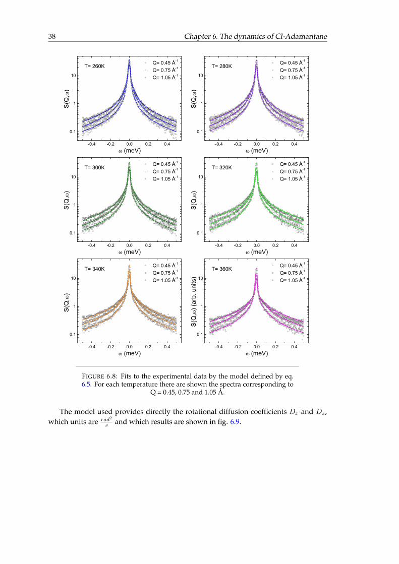
FIGURE 6.8: Fits to the experimental data by the model defined by eq.6.5. For each temperature there are shown the spectra corresponding to

Q = 0.45, 0.75 and 1.05 Å.

The model used provides directly the rotational diffusion coefficients Dx and Dz ,which units are rad2

s and which results are shown in fig. 6.9.


300 3600.000

0.001

0.002

0.003

0.02

0.03

0.04

0.05

0.06

Rot

atio

nal D

iff. C

oeffi

cien

ts

T (K)

Dx

Dz

FIGURE 6.9: Plot of the resulting Γ parameters with the model describedby eq. 6.5 for all the temperatures measured.

The rotational diffusion coefficients values obtained differ about one order of mag-nitude, what means that the rotational diffusion around x axis is much faster thanaround z axis. Another feature that can be concluded from fig. 6.9 is that rotationaldiffusion around x axis increases proportionally with the temperature. However, ro-tational diffusion around z axis seems not to be affected by temperature, at least untiltemperature reaches the highest values, when it is appreciated a slightly increment inthe Dz rotational diffusion coefficient. In fact, this phenomenon is better appreciated ifwe look at the degree of anisotropy δ which gives the quotient between the two rota-tional diffusion coefficients, δ = Dz

Dx. Fig. 6.10 shows clearly how the anisotropy of the

molecular movement changes at temperatures around 340 K.

300 3600.025

0.030

0.035

0.040

0.045

Dz/D

x

T (K)

FIGURE 6.10: Degree of anisotropy δ = Dz

Dxfor all the temperatures mea-

sured.


6.4 Conclusions

Bayesian analysis of the experimental data has been used to prove how many dynamicprocesses better describe the results obtained from the quasielastic neutron scatteringexperiment performed on Cl-adamante, in its plastic phase temperature range. Themodel selection through χ2 PDFs concludes that 2 processes are a better hypothesisthan 3, something that could not have been conclude by a frequentist approaching.

A fitting which a model, which consider the Cl-adamante as an oblong shapedmolecule, has allow to calculate the rotational diffusion coefficients Dx and Dz . Thisanalysis also allows to conclude that while the rotation around x axis increases propor-tionally with the temperature, the rotational diffusion around z does not behave in thesame way. It remains constant for the lower temperatures measured, but it seems toincrease for temperatures higher than 340 K. An effect that is appreciated much betterwhen looking at the degree of anisotropy in function of the temperature. This phe-nomenon could be related with the anomalous calorimetric effect introduced at thebeginning of the chapter. Perhaps, the atypical evolution of the heat-capacity at tem-peratures around 310 K, could be related with the observed rotational diffusion activa-tion around z axes at similar temperatures.

Probably, it is necessary a deeper analysis in order to indeed understand the molec-ular dynamics occurring in the Cl-Adamantane plastic phase at the range of temper-atures of interest. It would also be necessary to define a more rigorous explanationfor the relation between the dynamic evolution found and the unexplained calorimet-ric effect. Nevertheless, we have set the way that the oblong molecule hypothesis is agood approaching and that has been possible due to performing an accurate Bayesiananalysis.

Bibliography

[1] K. Kobashi, T. Kyomen and M. Oguni J. Phys. Chem. Solids Vol. 59, No. 5,pp. 667-677 (1998).

[2] L. C. Pardo, M. Rovira-Esteva, S. Busch, J. F. Moulin and J. Ll. TamaritPhys. Rev. E 84 046711 (2011).

[3] L. C. Pardo, M. Rovira-Esteva, S. Busch, M. D. Ruiz-Martín J. Ll. Tamaritand T. Unruh e-print arXiv:0907.3711 (2009).

[4] L. C. Pardo, M. Rovira-Esteva, S. Busch, M. D. Ruiz-Martín and J. Ll.Tamarit J. Phys.: Conf. Ser. 325 012006 (2011).

[5] D. Monserrat, A. Vispa, L. C. Pardo, R. Tolchenov, S. Mukhopadhyay andF. Fernández-Alonso J. Phys.: Conf. Ser. 663 012009 (2015).

[6] J. P. Amoureux, M. Bée and J. L. Sauvajol Molecular Physics 45, 709-719(1982).

[7] M. Bée and J. P. Amoureux Molecular Physics Vol. 48, No. 1, 63-79 (1983).

[8] M. Foulon, T. Belgrand, C. Gors and M. More Acta Cryst. B45, 404-411(1989).

[9] D. S. Sivia and J. Skilling, Data Analysis: A Bayesian Tutorial (Oxford Uni-versity Press, New York, 2006).

[10] T. Bayes Phil. trans. Roy. Soc. London 53 370 (1764).

[11] N. Metropolis, A. Rosenbluth, M. Rosenbluth, A. Teller, and E. Teller, J.Chem. Phys. 21, 1087 (1953) .

[12] The latest version of the MANTID software package can be downloadedfree of charge from http://download.mantidproject.org/

[13] D. S. Sivia and C. J. Carlile J. Chem. Phys. 96 170-178 (1992).

[14] M. Bée, Quasielastic Neutron Scattering: Principles and Applications in SolidState Chemistry, Biology and Materials Science (Adam Hilger, Bristol andPhiladelphia, 1988).

[15] G. L. Squires, Introduction to the Theory of Thermal Neutron Scattering(Cambridge University Press, Cambridge, 1978).

[16] B. T. M. Willis and C. J. Carlile, Experimental Neutron Scattering, (OxfordUniversity Press, Oxford, 2009).

[17] V. F. Sears Can. J. Phys. Vol. 44 (1966).

41

http://download.mantidproject.org/

42 BIBLIOGRAPHY

[18] S. Mukhopadhyay 2014 Rutherford Appleton Laboratory Technical ReportRAL-TR-2014-005 (Didcot, UK, 2014).

[19] V. García-Sakai, M. A. Adams, W. S. Howells, M. T. F. Telling, F. Demmeland F. FernÁndez-Alonso Rutherford Appleton Laboratory Technical ReportRAL-TR-2011-004 (Didcot, UK, 2011).

[20] G. Hinze, G. Diezemann, and T. Basché Phys. Rev. Lett. 93, 203001 (2004).

implementation of a bayesian algorithm into mantid for the

Documents