Implementation & Design of Physical Radar

Waveform Diversity

John Jakabosky, IEEE Graduate Student Member, Patrick McCormick, IEEE Graduate

Student Member, Shannon D. Blunt, IEEE Fellow

The authors are with the Electrical Engineering & Computer Science Dept., Radar Systems & Remote

Sensing Lab, University of Kansas, Lawrence, KS.

I. INTRODUCTION

Echo-locating mammals have been exploiting waveform diversity (WD) for about 50

million years [1], and the notion of radar waveform design has been around for several decades

(see [2] and references therein). However, the current instantiation of WD was first popularized in

2002 in the hopes of addressing the growing competition for radar spectrum [3]. Since that time,

there has been a tremendous amount of work on myriad aspects of WD (e.g. [4]), with a particular

emphasis on leveraging higher dimensionality (e.g. multiple-input multiple-output, or MIMO).

Much of this work has focused on the complex mathematical modeling and subsequent

optimization of radar “waveforms” (noting that the term tends to be used rather loosely). Here we

summarize recent work that seeks to connect the parameterized mathematical abstraction of radar

codes, which provide the benefit of being readily optimizable, with the physical attributes and

limitations of real radar systems and phenomenology. This physical perspective permits

realization of the promised performance enhancements of WD on actual hardware, as well as

providing the means with which to address radar spectrum issues for real systems.

Fundamentally, a radar waveform is a modulation of the transmitted signal in such a way

that, when the received echoes are match filtered (or at least minimally mismatched) to the

waveform, a processing gain is achieved that helps to separate the echoes from noise and to

distinguish the echoes from one another. This process is generally known as “pulse compression”

and decades of contributions have included a litany of waveform and filter design approaches [2].

2

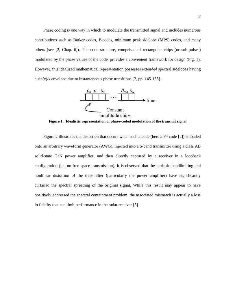
Phase coding is one way in which to modulate the transmitted signal and includes numerous

contributions such as Barker codes, P-codes, minimum peak sidelobe (MPS) codes, and many

others (see [2, Chap. 6]). The code structure, comprised of rectangular chips (or sub-pulses)

modulated by the phase values of the code, provides a convenient framework for design (Fig. 1).

However, this idealized mathematical representation possesses extended spectral sidelobes having

a sin(x)/x envelope due to instantaneous phase transitions [2, pp. 145-155].

Figure 1: Idealistic representation of phase-coded modulation of the transmit signal

Figure 2 illustrates the distortion that occurs when such a code (here a P4 code [2]) is loaded

onto an arbitrary waveform generator (AWG), injected into a S-band transmitter using a class AB

solid-state GaN power amplifier, and then directly captured by a receiver in a loopback

configuration (i.e. no free space transmission). It is observed that the intrinsic bandlimiting and

nonlinear distortion of the transmitter (particularly the power amplifier) have significantly

curtailed the spectral spreading of the original signal. While this result may appear to have

positively addressed the spectral containment problem, the associated mismatch is actually a loss

in fidelity that can limit performance in the radar receiver [5].

3

Figure 2: Spectral content of phase-coded modulation before and after the transmitter [6]

As elaborated in [6], it is thus useful to clarify the distinction between the terms code,

waveform, and emission. The code consists of a finite set of sequential phase values 0[ , , ] N

pertaining to some implementation structure (e.g. idealistic rectangular chips). In contrast, the

waveform is a continuous modulating signal whose spectral content is relatively amenable to the

natural bandlimiting imposed by the transmitter. Perhaps the most well-known waveform is the

linear frequency modulated (LFM) chirp [2, pp. 57-61], along with many variants of nonlinear

FM waveforms (e.g. [7-12]). Finally, the emission is defined as the physical signal launched into

free space by the radar, inclusive of transmitter distortion effects, non-instantaneous pulse

rise/fall-times (if pulsed), and electromagnetic coupling effects from the antenna and radar

platform (this effect is most pronounced for MIMO emissions [13]).

To achieve the promised sensing enhancements and spectral containment of WD, one must

consider the physical emission launched from the radar. Further, to achieve the benefits of

optimal/adaptive waveform-domain receive processing necessitates sufficient fidelity [14,15] that

can only be obtained by leveraging a loopback capture of the physical emission. The following

describes an implementation of polyphase codes as transmitter-amenable waveforms based on the

continuous phase modulation (CPM) scheme previously used in communications [16]. The

4

resulting polyphase-coded FM (PCFM) waveforms [6] are readily implementable on high-power

radar systems, yet can be optimized like codes [14]. By extension, this same framework permits

inclusion of transmitter distortion so as ultimately to enable optimization of the free space radar

emission [14]. Recent work on the extension to fast-time polarization modulation [17] and spatial

modulation [18,19] is also reviewed, including generalization to encompass both into a multi-

dimensional physical emission structure. Such higher dimension structure may permit enhanced

interference avoidance/suppression, particularly when combined with appropriate adaptive

processing on receive by exploiting the increased degrees of freedom.

II. POLYPHASE-CODED FM (PCFM)

The implementation of PCFM waveforms is achieved through a modification to the CPM

structure [16] that has been used for aeronautical telemetry, deep space communications, and the

BluetoothTM

wireless standard. For a pulsed radar emission [6], a train of N consecutive

impulses with time separation pT are formed such that the total pulsewidth is pT NT . The thn

impulse is weighted by n , the phase change between successive chips of the polyphase code is

determined by

if

2 sgn if

n nn

n n n

, (1)

where 1n n n for 1, ,n N , sgn( ) is the sign operation, and n is the phase value of

the thn chip in the length 1N polyphase code. The stipulations on the shaping filter ( )g t are

1) that it integrates to unity over the real line; and 2) that it has time support on [0, ]pT . For

example, rectangular filter meets these requirements (as do others). The sequence of phase

changes are collected into the vector x = [ 1 2 N ]T to parameterize the complex baseband

PCFM waveform as [6]

5

0

10

( ; ) exp ( ) ( 1)

t N

n p

n

s t j g n T d

x , (2)

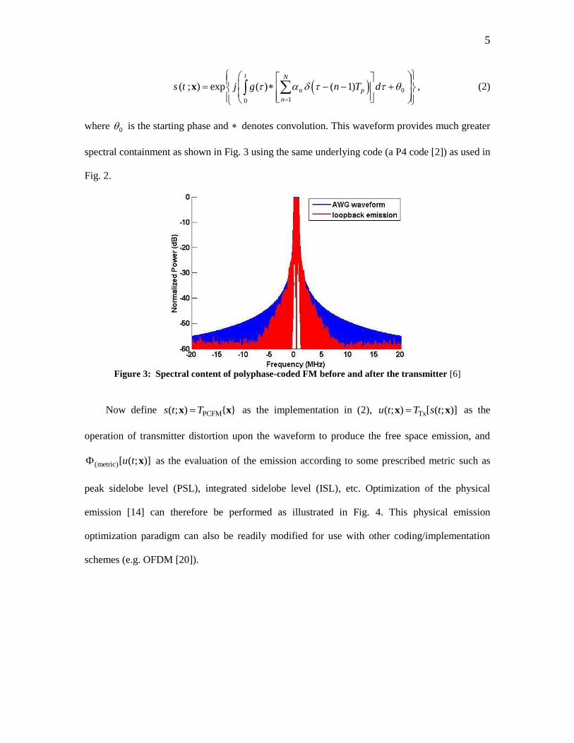
where 0 is the starting phase and denotes convolution. This waveform provides much greater

spectral containment as shown in Fig. 3 using the same underlying code (a P4 code [2]) as used in

Fig. 2.

Figure 3: Spectral content of polyphase-coded FM before and after the transmitter [6]

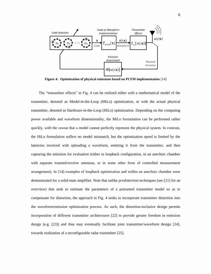
Now define PCFM( ; ) { }s t Tx x as the implementation in (2), Tx( ; ) [ ( ; )]u t T s tx x as the

operation of transmitter distortion upon the waveform to produce the free space emission, and

(metric)[ ( ; )]u t x as the evaluation of the emission according to some prescribed metric such as

peak sidelobe level (PSL), integrated sidelobe level (ISL), etc. Optimization of the physical

emission [14] can therefore be performed as illustrated in Fig. 4. This physical emission

optimization paradigm can also be readily modified for use with other coding/implementation

schemes (e.g. OFDM [20]).

6

Figure 4: Optimization of physical emissions based on PCFM implementation [14]

The “transmitter effects” in Fig. 4 can be realized either with a mathematical model of the

transmitter, denoted as Model-in-the-Loop (MiLo) optimization, or with the actual physical

transmitter, denoted as Hardware-in-the-Loop (HiLo) optimization. Depending on the computing

power available and waveform dimensionality, the MiLo formulation can be performed rather

quickly, with the caveat that a model cannot perfectly represent the physical system. In contrast,

the HiLo formulation suffers no model mismatch, but the optimization speed is limited by the

latencies involved with uploading a waveform, emitting it from the transmitter, and then

capturing the emission for evaluation (either in loopback configuration, in an anechoic chamber

with separate transmit/receive antennas, or in some other form of controlled measurement

arrangement). In [14] examples of loopback optimization and within an anechoic chamber were

demonstrated for a solid-state amplifier. Note that unlike predistortion techniques (see [21] for an

overview) that seek to estimate the parameters of a presumed transmitter model so as to

compensate for distortion, the approach in Fig. 4 seeks to incorporate transmitter distortion into

the waveform/emission optimization process. As such, the distortion-inclusive design permits

incorporation of different transmitter architectures [22] to provide greater freedom in emission

design (e.g. [23]) and thus may eventually facilitate joint transmitter/waveform design [24],

towards realization of a reconfigurable radar transmitter [25].

7

The optimization framework in Fig. 4 also implies a search process over the code space of

NL possibilities, where L is the number of possible phase changes. Noting that N closely

approximates the waveform time-bandwidth product (BT) and L 2, the dimensionality of this

search space can clearly be quite large. There are myriad approaches one may take to perform this

search [26]. In [14] a greedy search was employed by leveraging the observations that: 1) the

range-Doppler ambiguity function of the emission integrates to a constant (i.e. a “conservation of

ambiguity”); 2) chirp-like waveforms effectively absorb much of the range-Doppler ambiguity

into the well-known range-Doppler ridge; and 3) metrics that are based on attributes of the range-

Doppler ambiguity function (such as the zero-Doppler cut, otherwise known as the

autocorrelation) are complementary measures of the sidelobe levels. From these observations

emerged the performance diversity approach [14] that uses a chirp as initialization and alternates

between different metrics such as PSL and ISL during a greedy search to help avoid local

minima.

Consider an example of waveform optimization when using the mathematical model for the

distortion induced by a traveling wave tube (TWT) power amplifier [27]. The injected waveform

( ; )s t x is first filtered using a 4th order Chebychev filter having a 3-dB passband that is 2.4 times

greater than that of the PCFM waveform. This stage is used to model the linear transmitter effects

prior to the power amplifier. Denoting the resulting signal that is fed into the TWT as in ( ; )s t x ,

the amplified output signal is thus [27]

out in in in( ; ) ( ; ) | ( ; )| exp | ( ; )|s t s t A s t j s tx x x x (3)

where the terms

2

1

1 a

A rr

and 2

21

a rr

r

8

dictate the degree of amplitude and phase distortion, respectively, for a the amplitude-to-phase

modulation term, and 2s1a A for sA the saturating amplitude.

The time-bandwidth product (BT) for this example is 100 ≈ N, for B the 3-dB bandwidth.

First the PCFM waveform is optimized using the performance diversity approach [14] under the

assumption of an idealistic transmitter (no distortion). This optimized FM waveform realizes a

PSL of 43.8 dB and an ISL of 26.8 dB. Note that this value of PSL is actually 0.8 dB better

than the hyperbolic FM bound [9], which is a useful performance benchmark for constant

amplitude FM waveforms.

Two regimes of distortion are then examined using the above model with a set to /12

per [27] and the value 2sA set to 0 dB and 10 dB, representing mild and severe distortion,

respectively. Figure 5 illustrates the 2s 0A dB case (mild distortion). Specifically, the distorted

waveform has a PSL of 41.4 dB and ISL of 24.9 dB, corresponding to sensitivity losses of 2.4

dB and 1.9 dB, respectively. However, using the TWT model within the optimization process

yields a PSL of 42.4 dB and an ISL of 25.0 dB, i.e. a recovery of 1.0 dB and 0.1 dB,

respectively.

9

Figure 5: Model-in-the-Loop optimization for a TWT power amplifier (mild distortion)

In contrast, Fig. 6 illustrates the 2s 10A dB case (severe distortion). Now the distorted

waveform yields a PSL of 34.2 dB and an ISL of 18.8 dB, corresponding to sensitivity losses

of 9.6 dB and 8.0 dB, respectively. When MiLo optimization is applied using the TWT model the

resulting PSL attained is 38.8 dB and the ISL is 20.1 dB, i.e. a recovery of 4.6 dB and 1.3 dB

of lost sensitivity, respectively.

10

Figure 6: Model-in-the-Loop optimization for a TWT power amplifier (severe distortion)

Clearly, the incorporation of known transmitter distortion effects into the emission

optimization can compensate for some, but not all, of the sensitivity loss. However, an

appropriate hybridization between MiLo/HiLo optimization and traditional transmitter

predistortion [21] could potentially serve as a means to outperform either acting alone. More

generally speaking, this holistic perspective also provides the means with which to realize various

forms of waveform-diverse emissions in a manner that is physically realizable. Examples of this

holistic waveform diversity notion are provided in the next sections.

III. PCFM-BASED POLARIZATION MODULATION

Polarization diversity is widely used in weather radar [28] and synthetic aperture radar

(SAR) [29] to improve performance by capturing more information about the sensed

environment. The PCFM waveform implementation described in the previous section can be

extended to enable fast-time polarization modulation [17] via the incorporation of a hybrid

coupler along with an additional waveform. Denoting the two waveforms injected into the input

ports of the hybrid coupler as 1( )s t and 2 ( )s t , the resulting emissions from the horizontal (H) and

vertical (V) antennas to which the coupler is connected are

11

H 2 1

V 2 1

1( ) ( ) ( )

2

1( ) ( ) ( ) exp

2

s t s t s t

s t s t s t j

, (4)

where is an additional phase term used to select the particular great circle on the Poincaré

sphere (Fig. 7) upon which polarization modulation may occur.

Figure 7: Feasible polarization modulation regions on the Poincaré sphere for (left) = 0

and (right) = /2. RCP: right-hand circular, LCP: left-hand circular, LHP: linear

horizontal, LVP: linear vertical, L-45: linear with 45 tilt, L+45: linear with +45 tilt

To control the polarization state in fast-time using the PCFM structure, two length 1N

polyphase codes are required. The code 0 1, , , N is the same as used in (1) and (2) to

construct the length N phase-change sequence 1 2, , , N that controls the waveform phase

trajectory, noting that . Denote the second length 1N sequence as 0 1, , , N ,

for / 2 / 2 , which controls the polarization state upon a given great circle of the

Poincaré sphere. Defining a polarization state change sequence in the same manner as (1) yields

if / 2

sgn if / 2

nn

n

n n n

, (5)

where 1n n n for 1, ,n N .

12

Collect the polarization state change sequence into the vector p 1 2[ ]TN x and, to

avoid confusion, relabel the waveform phase-change vector used in (2) as w 1 2[ ]TN x .

Thus, in the same manner as (2), a polarization modulating signal can now be defined as

p 0

10

( ; ) exp ( ) ( 1)

t N

n p

n

p t j g n T d

x . (6)

Fast-time joint waveform/polarization modulation via the hybrid coupler is thus achieved with the

waveforms [17]

1 w p w p

0 0

10

12 w p w p

0 0

10

( ; , ) ( ; ) ( ; )

exp ( ) ( ) ( 1)

( ; , ) ( ; ) ( ; )

exp ( ) ( ) ( 1)

t N

n n p

n

t N

n n p

n

s t s t p t

j g n T d

s t s t p t

j g n T d

x x x x

x x x x

. (7)

Note that the differences between these two waveforms are the phase change sequences

( )n n and ( )n n along with the initial phase values 0 0( ) and 0 0( ) . When

combined in the hybrid coupler via (4) the result is to maintain the desired waveform from (2),

overlaid with the desired fast-time polarization modulation. Thus a new physically realizable

form of emission control can be achieved. Further details on this emission scheme and associated

receive processing can be found in [17].

III. PCFM-BASED JOINT SPATIAL & POLARIZATION MODULATION

The PCFM implementation can also be extended to perform fast-time spatial modulation

[18,19] which is a physically realizable form of MIMO radar that is relatively robust to errors

induced by mutual coupling [13] and avoids the fluctuations in voltage standing wave ratio

(VSWR) that can otherwise occur for MIMO [30]. In [18] and [19] the 1D and 2D instantiations

13

of spatial modulation were developed, respectively. The inspiration for these schemes is

fixational eye movement (FEM) of the human eye, where the “jittering” of the eye has been

linked to visual acuity. Thus, such a capability for radar may potentially have application to some

form of tracking. Here the notion of spatial modulation is combined with the polarization

modulation scheme of the previous section to realize joint Waveform/Spatial/Polarization (WaSP)

modulation as a high dimensional emission structure that may permit enhanced interference

avoidance/suppression while also facilitating greater information extraction from the sensed

environment (particularly when combined with adaptive receive processing).

Figure 8: Uniform planar array geometry

Consider a uniform planar array with half-wavelength spacing (Fig. 8) in which, relative to

array boresight, azimuth and elevation are measured as the angles az and el , respectively. With

(0,0) defined as the center of the array, the array elements are indexed as

( 1) / 2, ( 1) / 2 1, ... , ( 1) / 2

( 1) / 2, ( 1) / 2 1, ... , ( 1) / 2

x x x x

z z z z

m M M M

m M M M

(8)

where xM and zM are the number of horizontal and vertical array elements, respectively. To

perform 2D fast-time spatial modulation, two additional length 1N codes are needed. Define

these codes as az,0 az,1 az,, , , N and el,0 el,1 el,, , , N . Thus, again using the PCFM

phase-change framework and making the assumption that the spatial modulation does not “wrap

around” the endfire array directions, the spatial phase-change sequences are obtained as [18,19]

14

, az,c az, el,c el, az,c az, 1 el,c el, 1

, el,c el, el,c el, 1

2 2sin cos sin cos

2sin sin

x n n n n n

z n n n

d d

d

, (9)

for az,c and el,c the azimuth and elevation center look directions, respectively.

Collecting the spatial phase-change sequences into the vectors s, ,1 ,2 ,[ ]Tx x x x N x

and s, ,1 ,2 ,[ ]Tz z z z N x then provides the means to realize a spatially modulating signal

using the PCFM structure as [18,19]

s, , ,0

10

s, , ,0

10

( ; ) exp ( ) ( 1)

( ; ) exp ( ) ( 1)

t N

x x x n p x

n

t N

z z z n p z

n

b t j g n T d

b t j g n T d

x

x

, (10)

where az,c,0 az,0 el,c el,0

2sin cosx

d

and ,0 el,c el,0

2sinz

d

are the

initial azimuth and elevation modulation phases. Assuming each element location in the x zM M

planar array contains a horizontally polarized element and a vertically polarized element, with

each pair of these horizontal/vertical elements being connected to a hybrid coupler, then the

2 x zM M driving waveforms are

1, , w p s, s, w p s, s,

0

10

12, , w p s, s, w p s,

( ; , , , ) ( ; ) ( ; ) ( ; ) ( ; )

exp ( ) ( , ) ( 1) ( , )

( ; , , , ) ( ; ) ( ; ) ( ; )

x z

x z

x

x z

m mm m x z x x z z

t N

n x z p x z

n

mm m x z x x

s t s t p t b t b t

j g m m n T d m m

s t s t p t b t b

x x x x x x x x

x x x x x x x

s,

0

10

( ; )

exp ( ) ( , ) ( 1) ( , )

zmz z

t N

n x z p x z

n

t

j g m m n T d m m

x

(11)

where

15

, ,

0 0 0 ,0 ,0

, ,

0 0 0 ,0 ,0

( , )

( , )

( , )

( , )

n x z n n x x n z z n

x z x x z z

n x z n n x x n z z n

x z x x z z

m m m m

m m m m

m m m m

m m m m

(12)

according to the element indices xm and zm . Note, from (11), that this high-dimensional

emission can be decomposed into only four waveforms if the RF hardware permits sufficient

freedom in how they can be combined. While the structure in (11) appears to be rather

complicated, it is worth noting that the resulting emission from each antenna element is still just

an FM waveform, albeit one that is determined from a high-dimensional coding.

Generalizing (4), the signal emitted from the ( , )x zm m element in the array is

H, , 2, , 1, ,

V, , 2, , 1, ,

1( ) ( ) ( )

2

1( ) ( ) ( ) exp

2

x z x z x z

x z x z x z

m m m m m m

m m m m m m

s t s t s t

s t s t s t j

(13)

where all the code dependencies have been suppressed for brevity. Thus the horizontally and

vertically polarized far-field emissions are

az el el

az el el

( , ) ( )

H az el H, ,

( , ) ( )

V az el V, ,

1, , ( )

1, , ( )

x x z z

x z

x z

x x z z

x z

x z

j k m k m

m m

x z m m

j k m k m

m m

x z m m

g t s t eM M

g t s t eM M

, (14)

in which az el2 sin( )cos( ) /xk d and el2 sin( ) /zk d , for the wavelength of the

center frequency. As described in [18] for spatial modulation alone, time-varying and time-

aggregated beampatterns can be readily determined for these far-field emissions.

Due to the difficulty with visualizing such a high-dimensional emission, consider the

following example in which spatial modulation is performed only in the azimuth direction for

10xM dual-polarized elements. The spatial modulation sweeps linearly over an interval of

16

±11.54 centered on boresight (this interval is first null to first null as defined for a stationary

beam). The waveform is a piecewise linear phase approximation to LFM (see [6]) with BT = 50.

Likewise, the polarization modulation (using =0) performs four rotations around the Poincaré

sphere during the pulsewidth, beginning at horizontal polarization. This particular great circle

corresponds to the left side of Fig. 7 and includes linear horizontal and vertical and left-hand and

right-hand circular (and all polarization states in between these).

It is observed in the time-varying beampattern in Fig. 9 that the horizontally and vertically

polarized components sweep spatially across the boresight direction during the pulsewidth, while

the polarization modulation produces an offset lobing effect between H and V. Figure 10 shows

that this particular polarization modulation produces an aggregate beampattern that is nearly

identical between H and V, with both revealing the lower broadened peak that arises from spatial

modulation [18].

This example demonstrates some of the freedom that is available for emission design as

there are numerous different waveform/spatial/polarization modulation combinations that could

be realized for all manner of radar modalities. It remains to be seen how different multi-

dimensional emission structures can be designed for various sensing applications, though it

should be noted that such higher dimensional signal representations are particularly beneficial

when combined with adaptive receive processing that can exploit all the degrees of freedom.

17

Figure 9: Time-varying beampattern for (left) horizontally polarized and (right) vertically

polarized components of a joint Waveform/Spatial/Polarization (WaSP) modulated emission

Figure 10: Aggregate beampattern over the pulsewidth for horizontally and vertically

polarized components of a joint Waveform/Spatial/Polarization (WaSP) modulated emission

CONCLUSIONS

Recent work leveraging continuous phase modulation (CPM) from communications has

enabled the vast array of radar codes previously developed to be physically implemented as

polyphase-coded FM (PCFM) waveforms. This implementation permits the inclusion of

transmitter distortion effects so as to optimize the physical emission launched from the radar.

Further, this formulation allows for generalization to multi-dimensional emissions possessing

both spatial and polarization modulation in fast-time over the radar pulsewidth. Ongoing work is

18

exploring how these emission structures could be incorporated into various sensing modes and

prospective benefits (or trade-offs) in so doing.

REFERENCES

[1] M. Vespe, G. Jones, and C.J. Baker, “Lesson for radar: waveform diversity in echolocating

mammals,” IEEE Signal Processing Magazine, vol. 26, no. 1, pp. 65-75, Jan. 2009. [2] N. Levanon and E. Mozeson, Radar Signals, John Wiley & Sons, Inc., Hoboken, NJ, 2004.

[3] H. Griffiths, L. Cohen, S. Watts, E. Mokole, C. Baker, M. Wicks, and S. Blunt, "Radar

spectrum engineering and management: technical and regulatory issues," Proc. IEEE, vol.

103, no. 1, pp. 85-102, Jan. 2015.

[4] M. Wicks, E. Mokole, S.D. Blunt, V. Amuso, and R. Schneible, Principles of Waveform

Diversity and Design, SciTech Publishing, 2010.

[5] A.M. Klein and M.T. Fujita, “Detection performance of hard-limited phase-coded signals,”

IEEE Trans. AES, vol. AES-15, no. 6, pp. 795-802, Nov. 1979.

[6] S.D. Blunt, M. Cook, J. Jakabosky, J. de Graaf, and E. Perrins, “Polyphase-coded FM

(PCFM) radar waveforms, part I: implementation,” IEEE Trans. Aerospace & Electronic

Systems, vol. 50, no. 3, pp. 2218-2229, July 2014.

[7] C.E. Cook, “A class of nonlinear FM pulse compression signals,” Proc. IEEE, vol. 52, no.

11, pp. 1369-1371, Nov. 1964.

[8] J.A. Johnston and A.C. Fairhead, “Waveform design and Doppler sensitivity analysis for

nonlinear FM chirp pulses,” IEE Proc. F – Communications, Radar & Signal Processing,

vol. 133, no. 2, pp. 163-175, Apr. 1986.

[9] T. Collins and P. Atkins, “Nonlinear frequency modulation chirps for active sonar,” IEE

Proc. Radar, Sonar & Navigation, vol. 146, no. 6, pp. 312-316, Dec. 1999.

[10] I. Gladkova, “Design of frequency modulated waveforms via the Zak transform,” IEEE

Trans. Aerospace & Electronic Systems, vol. 40, no. 1, pp. 355-359, Jan. 2004.

[11] E. De Witte and H.D. Griffiths, “Improved ultra-low range sidelobe pulse compression

waveform design,” Electronics Letters, vol. 40, no. 22, pp. 1448-1450, Oct. 2004.

[12] A.W. Doerry, “Generating nonlinear FM chirp waveforms for radar,” Sandia Report,

SAND2006-5856, Sept. 2006.

[13] G. Babur, P.J. Aubry, F. Le Chevalier, “Antenna coupling effects for space-time radar

waveforms: analysis and calibration,” IEEE Trans. Antennas & Propagation, vol. 62, no. 5,

pp. 2572–2586, May 2014.

[14] S.D. Blunt, J. Jakabosky, M. Cook, J. Stiles, S. Seguin, and E.L. Mokole, “Polyphase-

coded FM (PCFM) radar waveforms, part II: optimization,” IEEE Trans. Aerospace &

Electronic Systems, vol. 50, no. 3, pp. 2230-2241, July 2014.

[15] D. Henke, P. McCormick, S.D. Blunt, and T. Higgins, "Practical aspects of optimal

mismatch filtering and adaptive pulse compression for FM waveforms," IEEE Intl. Radar

Conf., Arlington, VA, USA, May 2015.

[16] J.B. Anderson, T. Aulin, and C.-E. Sundberg, Digital Phase Modulation, Plenum Press,

New York, NY, 1986.

[17] P. McCormick, J. Jakabosky, S.D. Blunt, C. Allen, and B. Himed, "Joint

polarization/waveform design and adaptive receive processing," IEEE Intl. Radar Conf.,

Arlington, VA, USA, May 2015.

[18] S.D. Blunt, P. McCormick, T. Higgins, and M. Rangaswamy, “Physical emission of

spatially-modulated radar,” IET Radar, Sonar & Navigation, vol. 8, no. 12, Dec. 2014.

[19] P. McCormick and S.D. Blunt, "Fast-time 2-D spatial modulation of physical radar

emissions," Intl. Radar Symp., Dresden, Germany, June 2015.

19

[20] J. Jakabosky, L. Ryan, and S.D. Blunt, “Transmitter-in-the-loop optimization of distorted

OFDM radar emissions,” IEEE Radar Conference, Ottawa, Canada, Apr./May, 2013.

[21] F.M. Ghannouchi and O. Hammi, “Behavioral modeling and predistortion,” IEEE

Microwave Magazine, pp. 52-64, Dec. 2009.

[22] F.H. Raab, P. Asbeck, S. Cripps, P.B. Kenington, Z.B. Popovic, N. Pothecary, J.F. Sevic,

and N.O. Sokal, “Power amplifiers and transmitters for RF and microwave,” IEEE Trans.

Microwave Theory & Techniques, vol. 50, no. 3, pp. 814-826, Mar. 2002.

[23] L. Ryan, J. Jakabosky, S.D. Blunt, C. Allen, and L. Cohen, "Optimizing polyphase-coded

FM waveforms within a LINC transmit architecture," IEEE Radar Conf., Cincinnati, OH,

May 2014.

[24] H. Griffiths, S. Blunt, L. Cohen, and L. Savy, “Challenge problems in spectrum

engineering and waveform diversity,” IEEE Radar Conf., Ottawa, Canada, Apr./May 2013.

[25] M. Fellows, M. Flachsbart, J. Barlow, J. Barkate, C. Baylis, L. Cohen, R.J. Marks,

“Optimization of power-amplifier load impedance and waveform bandwidth for real-time

reconfigurable radar,” IEEE Trans. Aerospace & Electronic Systems, vol. 51, no. 3, pp.

1961-1971, July 2015.

[26] C. Blum and A. Roli, “Metaheuristics in combinatorial optimization: overview and

conceptual comparison,” ACM Computing Surveys, vol. 35, no. 3, pp. 268-308, Sept. 2003.

[27] E. Costa, M. Midrio, and S. Pupolin, "Impact of amplifier nonlinearities on OFDM

transmission system performance," IEEE Communications Letters, vol. 3, no. 2, pp. 37-39,

Feb. 1999.

[28] V.N. Bringi and V. Chandrasekar, Polarimetric Doppler Weather Radar: Principles and

Applications, Cambridge, U.K.: Cambridge Univ. Press, 2001.

[29] J.J. van Zyl and Y. Kim, Synthetic Aperture Radar Polarimetry, John Wiley & Sons, Inc.,

Nov. 2011.

[30] Daum, F., Huang, J., “MIMO radar: snake oil or good idea?” IEEE AES Mag., May 2009.