information theory and radar waveform designmrb/resources/selpubsf/itradarwaveforms.pdfdetection of...

1578 IEEE TRANSACTIONS ON INFORMATION THEORY, VOL. 39, NO. 5, SEPTEMBER 1993

Informa tion Theory and Radar Waveform Design Mark R. Bell

Abstract-The use of information theory to design waveforms for the measurement of ex tended radar targets exhibiting resonance phenomena is investigated. The target impulse response is introduced to model target scattering behavior. Two radar waveform design problems with constraints on waveform energy and durat ion are then solved. In the first, a deterministic target impulse response is used to design waveform/receiver-fi lter pairs for the opt ima1 detection of ex tended targets in additive noise. In the second, a random target impulse response is used to design waveforms that maximize the mutual information between a target ensemble and the received signal in additive Gaussian noise. The two solutions are contrasted to show the difference between the characteristics of waveforms for ex tended target detection and information extraction. The optimal target detection solution places as much energy as possible in the largest target scattering mode under the imposed constraints on waveform durat ion and energy. The optimal information extraction solution distributes the energy among the target scattering modes in order to maximize the mutual information between the target ensemble and the received radar waveform.

Index Terms-Mutual information, radar, matched filter, radar waveforms, target impulse response, ex tended radar targets, target scattering resonance, ul tra-wideband radar.

I. INTRODUCTION

S HORTLY after the publication of Shannon’s A Muthe- matical Theory of Communication [l] in 1948, Woodward

and Davies began investigating the application of information theory to radar [2]-[5]. In 1953, Woodward published the book Probability and Information Theory with Applications to Radar [6], in which he presented both an introductory tutorial of information theory from the viewpoint of radar detection as well as a summary of results from his investigations with Davies. From these works, it is apparent that, at its inception, information theory was considered applicable to radar problems, particularly in the area of radar detection. The rationale behind these early investigations of the application of information theory to radar problems was summarized by Woodward [6, p. 621 as follows:

The problem of reception is to gain information from a mixture of signal and unwanted noise, and a considerable literature exists on the subject. Much of it has been concerned with methods of obtaining as large a signal- to-noise ratio as possible on the grounds that noise ultimately limits sensitivity and the less there is of it the better. This is a valid attitude as far as it goes,

Manuscript received June 14, 1990; revised December 28, 1992. This work was supported by Hughes Aircraft Company and by the National Science Foundation under Research Initiation Award MIP-9010834.

The author is with the School of Electrical Engineering, Purdue University, West Lafayette, IN 47907.

IEEE Log Number 9211657.

but it does not face up to the problem of extracting information. Sometimes it can be misleading, for there is no general theorem that maximum output signal-to-noise ratio insures maximum gain of information.

In their work, Woodward and Davies use information-theoretic ideas to formulate the a posteriori radar receiver, which in the case of bandlimited additive white Gaussian noise results in the correlation receiver. They did not, however, extend the rationale noted above to the problem of radar waveform design for the purpose of extracting information about a target.

Since the time of Woodward’s and Davies’ investigations, a few researchers have considered the relationship between information theory and radar detection and estimation problems, but none of them have considered the use of information theory in radar waveform design. Frost and Shanmugan [7] examined the use of information theory in order to calculate the information content of synthetic aperture radar images. They then used the information content of synthetic aperture radar images generated using noncoherent integration with a variable number of looks in order to determine a measure of radiometric resolution. W ilcox [8] considered the problem of designing waveforms from the radar ambiguity function for narrowband signals. Naparst [9] recently investigated the problem of wideband waveform design and processing to resolve targets in dense target environments. None of these investigations, nor any others that could be found, addressed the issue of using mutual information in the design of radar waveforms and processing.

In this paper, we consider the problems of radar waveform design for optimal target detection (maximum output signal-to- noise ratio) and optimal target information extraction, when the radar targets are modeled as extended radar targets. Extended radar targets are targets of significant physical extent, so they no longer behave as simple point targets which scatter a scaled and attenuated version of the transmitted waveform back to the radar receiver, but instead they exhibit interference and resonance effects in the scattered electric field as a result of the target’s physical extent.

The first problem, that of waveform design for the optimal detection of radar targets that exhibit resonance phenomena, involves the design of radar waveforms and receiver-filters that maximize the output signal-to-noise ratio at the receiver-filter output under constraints on transmitted waveform energy and duration. The second problem deals with the design of radar waveforms which maximize the mutual information between an ensemble of extended targets and the receiver-filter output. The waveforms of this second problem will be shown to be optimal, in a certain sense, for characterizing or identifying the target under observation. As we will see, information theory

001&9448/93$03.00 0 1993 IEEE

BELL: INFORMATION THEORY AND RADAR WAVEFORM DESIGN 1579

provides a unique insight into the relative characteristics of the two families of waveforms that arise in the solution of these two problems.

The waveforms solved for by maximizing the mutual information between the random target ensemble and the received radar signal will be called information extraction waveforms or estimation waveforms. We call these waveforms estimation waveforms because of the relationship between mutual information and the lower bound on parameter error as expressed through the rate distortion function. We do not explicitly discuss parameter estimation with these waveforms using standard parameter estimation techniques. Rather, the sense in which these are good estimation (or classification) waveforms is discussed in Section II-C.

In Section II, we formulate the problems of waveform design for target detection and target estimation. In formulating these waveform design problems, we will introduce the idea of target impulse response for both deterministic targets and random target ensembles. The target impulse response will allow us to represent the scattering characteristics of the radar target using an approach motivated by signal theory rather than electromagnetic scattering theory. We then formulate the two waveform design problems, considering the models that give rise to them and the rationale behind the optimality criteria used in formulating the problems.

In Section III, we summarize the major results obtained for both the detection waveform problem and the estimation waveform problem. In Theorem 1, we present an algorithm for the design of optimal waveform/receiver-filter pairs for detection of targets with known impulse response under constraints on waveform duration and energy. We also give the resulting signal-to-noise ratio obtained using the optimal waveform/receiver-filter pairs. In Theorem 2 we present the main result on estimation waveforms. Theorem 2 describes the spectral characteristics of waveforms that maximize the mutual information between a Gaussian target ensemble and the received radar waveform.

In Section IV, we solve the problem of finding the waveform/receiver-filter pair for optimal extended target detection and prove Theorem 1. In Section V, we consider the problem of designing optimal estimation waveforms and prove Theorem 2. In Section VI, we present examples of the design and performance of waveforms for both the optimal detection and estimation problems. We also compare the characteristics of the optimal detection and estimation waveforms. Finally, in Section VII, we summarize the results of our investigation.

II. FORMULATION OF PROBLEMS

A. Target Impulse Response

Radar targets are commonly modeled as point targets-targets of infinitesimal physical extent. The resulting simplification is that the reflected radar waveform observed at the receiver is an amplitude-scaled and time-delayed replica of the transmitted waveform. For narrow bandwidth waveforms, the point target model is often valid, but as the waveform bandwidth Af becomes comparable to c/2Az, where c is the

speed of light and AZ is the spatial extent of the radar target in range, the point-target model does not accurately reflect the behavior of radar scatterers. As AZ becomes comparable to c/2Af, the return must instead be viewed as coming from several-or even a continuum-of points in an extended region of space. As a result, the received radar signal is the sum of multiple delayed versions of the transmitted waveform. Targets exhibiting such scattering behavior are called extended targets.

The propagation and scattering of electromagnetic waves, as they typically occur in radar measurement, are linear processes, obeying the principles of superposition and homo- geneity. One common method of studying linear processes such as scattering is to view’ them as linear systems and to study the input/output relationships of their representative linear systems. In addition to being linear, the system may also be time-invariant, as would be true if the target was stationary with respect to the radar. The system impulse response is then a convenient tool for characterizing the input/output relationships of the system.

To apply linear systems analysis to scattering problems, we will first define the input and output quantities to be the electric field present at a pair of points in space. We will assume a fixed, although not necessarily identical, polarization at each point. The input e(t) is the 3 polarized electric field at point Pr. We assume that the plane wave is propagating along the line connecting Pr and the origin. If the plane wave is incident on the target located at the origin, a scattered electric field will be present at an arbitrarily chosen observation point Pz. We select an arbitrary polarization f’ at P2 and view as the output of our linear system the electric field v(t) at point P2 with polarization P’. Thus, restricting the direction and polarization of the incident plane wave and selecting a point P2 for measurement of the scattered wave for a fixed polarization, we have that the relationship between e(t) and w(t) is that of a linear system. We will also assume that the scatterer is stationary during the period of observation, and that the system relating e(t) and w(t) is a linear time-invariant system.

We will designate the impulse response of this system by h(t). For general e(t), the output w(t) of the linear system is given by the convolution integral

w(t) = J O3 h(T)e(t - T) dr. -co

Let the Fourier transforms of e(t), w(t), and h(t) be given by E(f), V(f), and H(f), respectively. Then

V(f) = E(f)H(f). Although we have assumed that the target is stationary with

respect to the radar, this approach can be generalized for a wide class of targets in motion as well. For a wide class of target motions with respect to the radar (e.g., radial target motion in a monostatic radar system), the received waveform w(t) for the target in motion is the same as that for the stationary target, except with a contraction or dilation of the time-axis induced by the Doppler effect. Hence, the analysis can be generalized for target motion in much the same way that the matched filter is generalized for target motion in a standard radar processor.

1580 IEEE TRANSACTIONS ON INFORMAl’ION THEORY, VOL. 39, NO. 5, SEPTEMBER 1993

While a deterministic target impulse response may be useful in the case where the target of interest is known a priori, there are many instances where such a priori knowledge is not available. In such cases, it may be possible to approximate the target impulse response from known physical characteristics of the target under consideration, or else treat the target impulse response as a finite-energy random process. The former approach may be useful in the design of waveforms for optimal target detection, whereas the latter approach will be used in the problem of waveform design for target information extraction.

The random impulse response g(t) is a finite-energy random process used to model the scattering characteristics of a random target. The random process g(t) can be thought of as an ensemble {g(t, w)} of functions, where w E fl and R is the underlying sample space. We will now examine some properties of the random impulse response g(t).

The first property which g(t) must possess is that all of the sample functions g(t, w) must satisfy

r ~m19(w)12 Lit 5 1.

This follows from conservation of energy and the fact that electromagnetic scattering is a passive process. The next property of g(t) we will assume is that all of its sample functions are causal impulse responses; that is, g(t, w) = 0, Vt < 0, VW E R. This is a property of all physical linear time-invariant systems. In addition, we will also assume that the Fourier transform {G(f, w)} of each sample function {g(t, w)} exists. A sufficient condition for this is that each sample function {g(t, w)} have only finite discontinuities, ilong with the first condition on the sample functions given above [12]. W ith thesk conditions, the Fourier transform G(f) of g(t) exists.

Finally, we will assume that g(t) is a Gaussian random process. This is a reasonable assumption for targets consisting of a large number of scattering centers randomly distributed in space, since both the in-phase and quadrature components of the received signal in such cases are, at least approximately, Gaussian random processes.

Throughout the remainder of this paper, a deterministic target impulse response will be denoted h(t), while a random target impulse response will be denoted by the random process g(t).

B. Optimal Detection ,Waveforms

When detecting radar targets, the presence or absence of a target is generally determined by a threshold test on the energy in the received signal. When a target is present, we expect that there will be greater energy in the received signal than when no target is present.

As is well known from standard detection theory results, in order to obtain the best target detection performance in a radar using either a Neyman-Pearson or Bayes decision rule, the signal-to-noise ratio at the output of the radar receiver should be made as large as possible [13], [14]. It follows then that for optimal detection, we should design our waveform and

receiver to make the signal-to-noise ratio as large as possible under the physical constraints placed on the waveform and receiver.

The problem of interest can be stated as follows. Given a target impulse response h(t) and stationary additive Gaussian noise n(t) with power spectral density S,,(f), find a transmitted waveform x(t) with total energy E, and a receiver-filter impulse response r(t) such that the signal-to-noise ratio of the receiver output y(t) is maximized at time to. In addition, because real radar waveforms are of finite duration, restrict the waveform z(t) such that it is zero outside the interval [-T /2, T /21.

The primary difference between this problem and a standard matched filtering problem [II] is the effect of the target in changing the shape of the transmitted waveform in accordance with its scattering characteristics. The optimal receiver-filter itself should be matched to the waveform scattered by the target, not the transmitted waveform itself. But this alone is not sufficient in order to achieve the maximum attainable signal- to-noise ratio under the transmitted waveform constraints. We must find the waveforms meeting the constraints that, when filtered with the proper receiver-filter matched to the waveform scattered by the target, will yield the greatest signal-to-noise ratio.

C. Optimal Estimation Waveforms

A radar system may make measurements of a target in order to determine unknown characteristics of the target. Stated differently, we can say that a radar system may make measurements of a target in order to decrease the a priori uncertainty about the target. In the analysis of communication channels, information theory provides a method of quantifying the decrease in the apriori message uncertainty of the transmitted message by observing the channel output. Such an approach has successfully allowed for the information transmission capabilities of a communication channel to be determined. This being the case, let us examine the measurement process in general in light of information theory in order to determine the information transmitted to an observer by a measurement mechanism. These results then can be applied to the radar measurement problem.

Consider a measurement system in which we have an object to be measured, a measurement mechanism, and an observer. We assume that the random vector X consists of parameters characterizing the object we wish to measure and that a probabilistic model of the unknown parameters is meaningful. The measurement mechanism maps X into the random vector Y, and the observer observers Y. From this observation, the observer determines the desired description of X. The measuretnent mechanism is assumed to have inherent inaccuracies, so its measurements contain errors. This can be modeled by assuming that the measurement mechanism stochastically maps the random vector X E Rx to the random vector Y E Ry . We will denote the mutual information between X and Y to 1(X; Y).

The mutual information 1(X; Y) between two random vec- tors X and Y tells ut the quantity of information observation


of measurements, it is common to talk about the accuracy in terms of some error criterion, for example, mean-squared error of relative mean squared error. It would be useful if we could relate the mutual information 1(X; Y) to the relevant measurement error criterion. Rate distortion theory provides a framework for doing this.

In making a measurement, we are trying to obtain a description of the object parameter vector X from the measurement vector Y. Because of inaccuracies in the measurement process, we cannot generally obtain X perfectly, so there is an error associated with a given parameter vector z and a given ’ measurement vector y. Let us designate this error or distortion as d(z, y). We assume that this distortion is a nonnegative function defined for all pairs of x E Rx and y E Ry. The mean distortion S is the expectation of d(x, y). Thus,

6 = E{d(x, Y)>.

The rate distortion function R(D) for a single measurement is defined as

of Y provides about X; that is, 1(X; Y) is the amount of information that the measurement Y provides about the object parameter vector X. The greater this mutual information is, the greater the quantity of information describing the object we obtain from our measurement and the greater the reduction in the a priori uncertainty as a result of this measurement. Intuitively, we might expect that the greater the mutual information between a measurement and the quantity being measured, the more accurately we can classify or estimate the parameters characterizing the entity we are trying to measure. Berger alludes to this idea when he makes the statement: “Rate distortion theory provides knowledge about how the frequency of faulty categorization will vary with the number and quality of observations” [15, p. 91, since the rate distortion function relates the average distortion or error to the minimum mutual information required to achieve that error.

We shall justify the idea that the greater the mutual information between the parameter we are measuring and the measurement, the better our ability to classify or estimate the parameters describing the object, in two ways. We will determine the maximum number of equiprobable classes into which we can assign X by observation of Y; then we relate 1(X; Y) to the average measurement error through use of the rate distortion function. This is done in the following two propositions. We also cite a recent result relating to this problem [ 161.

Consider the problem of putting X into one of N equiprobable classes based on observation of Y. That is, assume that RX has been partitioned into N equiprobable subsets, and we wish to assign X to its proper subset based on observing the Y generated by the measurement process.

Proposition 1: For any decision rule assigning X to a subset of a partition based on observation of Y, and for all possible equiprobable partitions of Rx, the maximum number of partitions N for which this can be done with an arbitrarily small probability of error is

(1) To see that this is true, we note that, given 1(X; Y) =

10 nats, we can calculate the associated N, which we will designate No, as

No = [e’“] .

Then

No@‘<No+l.

Since the logarithm is a monotonically increasing function of its argument for all positive real numbers,

In NO < Ia < In (NO + 1).

By Shannon’s Theorem for the noisy channel, it is not possible to classify X into one of NO + 1 equiprobable classes. This cannot be done without the channel’s transferring In (No + 1) nats of information. But the measurement mechanism cannot possibly do so, because 10 < In (NO + 1).

We now consider the relationship between mutual information and measurement error. When examining the accuracy

R(D) =. min {1(X, Y): S 5 D}. (2)

The minimization is over all measurement mechanisms that satisfy the condition that the fidelity criterion S is less than or equal to D. The minimization may also be constrained to measurement mechanisms which satisfy a specified set of conditions (e.g., the condition that a single measurement can use at most EO joules of energy). The rate distortion function R(D) gives the minimum possible rate at which information must be transferred by a measurement mechanism in order to have an average error or distortion S less than or equal to D.

It is well known that R(D) is a nonincreasing function of D. So the smaller the average error D, the larger is the minimum required information rate R(D) required of the measurement mechanism in order to achieve this average error D. We summarize these ideas in the following proposition.

Proposition 2: Let D be the largest allowable mean error between the object parameter vector X and the measurement vector Y. Then the minimum possible value of 1(X; Y) for which D can be achieved is a nonincreasing function of D.

Intuitively, this makes sense. It says that if greater accuracy is required in the measurements, the measurement mechanism must provide more information about the object being measured.

In general, the greater the mutual information between the parameters we wish to measure and the measurements them- selves, the more we can say about the object being measured. In the case where we examined the ‘number of equiprobable classes to which we could assign X based on observation of Y, we saw that the larger 1(X; Y), the larger the number of classes. In the case of the rate distortion function, we saw that the more precise we wanted our measurements to be, the greater the minimum rate of information transfer by the measurement mechanism.

A recent result by Kanaya and Nakagawa [16] relates mutual information to Bayes risk in statistical decision problems in a mathematically rigorous manner. For a random parameter 0 taking on values from a finite parameter set, they define


I I - I

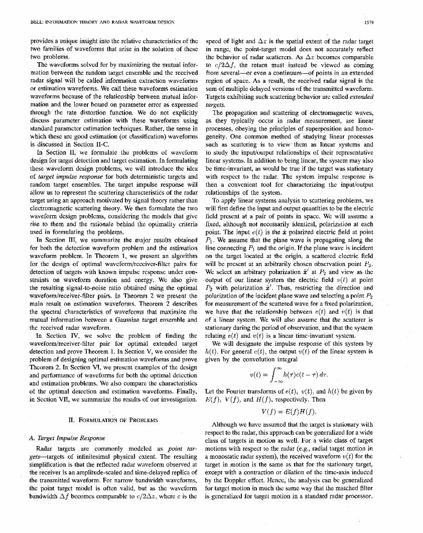
Fig. 1. Block diagram of the radar target channel.

a function R(P, L) that determines the minimum required mutual information between 0 and a measurement such that the Bayes risk is less than or equal to a value L given that

I the random parameter 0 has probability distribution P. This function is closely related to the rate distortion function. They then prove asymptotic results that show that for a sufficiently large number of independent experiments, the probability that the average Bayes loss is greater than L goes to zero as the number of experiments grows large, if the measurements associated with each experiment exceed R(P, L). This result, perhaps of limited practical importance in the design of statistical decision procedures; does point directly to the fact that the greater the mutual information between the parameter and its measurement, the better the expected performance in the best Bayes risk decision procedure.

In applying Propositions 1 and 2 to the measurement mechanism of radar, we see that if we design radar systems in such a way as to maximize the mutual information between the target parameters of interest and their measurements, then the better we can expect our system performance to be, at least if we measure system performance in terms of target classification ability or average measurement error. This being the case, we will consider optimal information extraction waveforms to be those waveforms that maximize the mutual information between the observed target ensemble and the output of the radar receiver. It is this class of waveforms, under the imposed duration and energy constraints, that ‘we are interested in finding.

Consider the radar target channel model shown in Fig. 1. Here, z(t), a finite-energy deterministic waveform with energy E, and of duration T is transmitted by’the transmitter in order to make a measurement of the radar target. We will assume that x(t) is confined to the symmetric time interval [-T/2, T/2]. Thus,

I T/2 E, = Ix(t)12 dt.

-T/2 (3)

Since the energy constraint in most real radar systems is not on, the total energy in the transmitted waveform, but rather on the average power of the waveform, we will be interested in the average power P,, which satisfies the relation E, = P,T. We also assume that x(t) is confined to a frequency interval W = [fa, fa + IV]. While strictly speaking, we cannot have an x(t) with finite support whose Fourier transform has finite support, we assume that W is selected so that only negligible energy resides outside the frequency interval W .

After transmission, the radar waveform x(t) is scattered by the target, which has a scattering characteristic modeled by the random impulse response g(t). The resulting scattered signal z(t) received at the receiver is a finite-energy random process,

and is given by the convolution integral

Z(t) = r

g(T)x(t - T) dr. -co

The random process z(t) is received at the receiver in the presence of the zero-mean additive Gaussian noise process n(t) . This noise process is assumed to be stationary and ergodic, and to have one-sided power spectral density P,,(f) = 2&,(f) for f > 0. In addition, n(t) is assumed to be statistically independent of both the transmitted waveform x(t) and the target impulse response g(t).

The waveform received at the receiver is shown in Fig. 1 to be z(t) + n(t) filtered by the ideal linear time-invariant bandpass filter B(f), passing only frequencies in the band W . The explicit inclusion of the filter B(f) is just a statement of the fact that we assume that the transmitted signal has no significant energy outside the frequency interval W . Thus, neither does z(t), since it is the response of a linear time- invariant system to the transmitted signal.

For a given sample function g(t, wa) with the Fourier transform G(f, wa), the resulting spectrum of the scattered signal z(t) is given by Z(f, wu) = X(f)G(f, we). The magnitude squared of this spectrum is ]Z(f, wa) 1’ = IX(f)121G(f, we)]“. Taking the expectation with respect to G(f), the mean-square spectrum of z(t) is

-WYf)12 = l~(f)12EW (f12~~ Now,

EW(f)12) = bG(f)12 + ddf), where ,&(f) is the mean of G(f) and 02 (f) is the variance of G(f); that is,

pG(f) = E{G(f)),

and

a&(f) = E-W (f) - pG(f)12).

We are interested primarily in a&(f) for the Gaussian target model, as the signal component of z(t) corresponding to the mean &!(f) is known since x(t) is known. It thus tells us nothing about the target. In most cases, ,&(f) = 0, since there is a random delay d in g(t) because of the target’s random position in space. This corresponds to a random phase factor of exp { -i2rfd}, which has expectation zero for a wide class of distributions on d. We will thus assume that ,UG(f) = 0.

Similarly, if we define

~z(f) = E{Z(f))

and

then

d(f) = ww - PZ(f12~~

vxf)12 = IPZ(f)12 f&f). Referring again to Fig. 1, we will assume that the radar

receiver observes y(t) for a period T in order to obtain

BELL: INFORMATION THEORY AND RADAR WAVEFORM DESIGN

information about the target. The duration of observation 5? must be long enough to allow the receiver to capture all but a negligible portion of the energy in the sum of the scattered signal z(t). We know that the duration of the transmitted waveform is T, and we known that z(t) must be at least this long, since the convolution of two waveforms of finite duration Tl and T2 produces a waveform of duration Tl + Tz. So if Tg is the duration of g(t) , then the duration of a(t) is T + Tg.

The received y(t) consists of the scattered signal z(t) and the additive Gaussian noise n(t) passed through the ideal bandpass filter B(f), p assing the frequency interval W . The impulse response hw (t) of this filter is

b(t) = w~cos (fo + W /2)k

The duration of this pulse is infinite, but, as is well known, most of the energy is concentrated in an interval of duration l/W . Thus, it is reasonable to assume the impulse response duration Tw of the ideal passband filter at the receiver to be Tw M l/W .

It is reasonable to assume that the bandwidth over which most radar targets exhibit significant scattering of electromagnetic waves is much larger than the bandwidth of the radar system used in order to make the scattering measurements [27, Section 27.61. Hence it is reasonable to assume

Tg < Tw.

Also, for most radar signals, the duration of the transmitted signal is much larger than l/W . This is often necessary to provide enough signal energy for reliable target detection. An example of this is the lienar FM or “chirp” signal commonly encountered in radar systems. This allows a range resolution equivalent to a much narrower pulse than that actually transmitted. Long transmission time, or “time-on-target” is also common in radar target recognition problems, where the longer observation time allows better frequency resolution in the measured Doppler spectrum. For such signals, the actual duration T of transmission is much larger than the l/W . For such systems, T > T W E l/W . So in summary, 5?’ = T + Tg + Tw % T + T W E T + l/W , and for systems that satisfy the condition T > l/W , 5? E T.

The problem of interest can now be stated as follows. Given a Gaussian target ensemble with random impulse response g(t) having spectral variance o&(f), find the waveforms x(t) confined to the symmetric time interval [-T/2, T/2] and having all but a negligible fraction of their energy confined in (one-sided) frequency to W = [fa, fe + W ] that maximize the mutual information I(y(t); g(t) I x(t)) in additive Gaussian noise with one-sided power spectral density P,,(f).

III. SUMMARY OF RESULTS

We now present the main results of our investigation as two theorems. Theorem 1 summarizes the main results on the design of waveform/receiver-filter pairs for optimal target detection. Theorem 2 summarizes the main results for the design of optimal estimation waveforms.

1583

A. Results on Detection Waveforms

The main results arising. from the solution of the waveform/receiver-filter design problem for optimal detection can be summarized in the following design algorithm, which explicitly states how to calculate the optimal waveform/receiver-filter pair, and gives an expression for the resulting signal-to-noise ratio.

Theorem 1: A waveform/receiver-filter pair maximizing the signal-to-noise ratio at the output of the receiver-filter can be designed using the following algorithm.

a> Compute

L(t) = s

O3 -cc

b)

Here 5&(f) is the two-sided power spectral density of the noise n(t), and h(t) is the impulse response of the target. Solve for an eigenfunction 2(t) corresponding to the maximum eigenvalue X,,, of the integral equation

s T/2 x,,q t) = ?(T)L(t - T) dr. -T/2

4 Scale 2(t) so that it has. energy E,. Compute the spectrum X(f) corresponding to the optimal waveform Z(t):

22(t) = r

?(t)e --i‘hft dt. -cc

4 Implement a receiver-filter of the form

R(f) = Kri-(f)H(f)e-i2Tfto Snn(f) ’

e> where K is a complex constant. The resulting signal-to-noise ratio for this design, which is the maximum obtainable under the specified constraints, is

= kn,x~%.

The proof of this result is given in Section IV.

B. Results on Estimation Waveforms

The main results arising from the solution of the optimal estimation waveform design problem can be summarized in the following theorem.

Theorem 2: If x(t) is a finite-energy waveform with energy E, confined to the symmetric time interval [-T/2, T/2], and having all but a negligible fraction of its energy confined to the frequency interval W = [fa, fe + W ], the mutual information I(y(t); g(t) I x(t)) between y(t) and g(t) in additive Gaussian noise with one-sided power spectral density P,,(f) is maximized by an x(t) with a magnitude-squared


spectrum

lX(f)12 = max 0, A - Pm(f )F % (f 1 1

= max [0, A - r(f)],

where r(f) = P,,(f)?/2a&(f), and A is found the equation

Lemma 1: A necessary condition for the maximization of the signal-to-noise ratio is

R(f) = KX(f)H(f)e-i2”f”o &n(f) ’

(4) and with R(f) satisfying the relation of (lo), signal-to-noise ratio is

by solving - ($), = [~‘x~n~j;)‘2df.

(5) Although (10) is a necessary and sufficient

achieve the maximum signal-to-noise ratio for

(11)

condition to a fixed x(t),

it is not sufficient to provide a waveform/receiver-filter pair

(10) the resulting

The resulting maximum value Imax(y(t);g(t) I x(t)) of (x(t), r(t)) that achieves the maximum possible signal-to-

W t);dt) I xc(t)> is noise ratio for all waveforms satisfying the imposed constraints. In order to do this, r(t) must satisfy (lo), but in addition, we must find a signal x(t) that maximizes (11) under the constraints

I -~[x(f)12df=Ez, CT s max [0, In A - In r( f)] df. (6)

W xc(t) = 0, for all t 6 [-T/2, T/2]. (12)

The proof of this result is given in Section V.

IV. WAVEFORMS FOR DETECTION OF EXTENDED TARGETS

We now show that the design procedure of Theorem 1 gives a waveform/receiver-filter pair that produces the largest possible signal-to-noise ratio for an extended target. The receiver output is given by

y(t) = Ys(4 + y,(t).

Here, ys(t) is the signal component in the receiver output, and yn (t) is the noise component in the receiver output. These two components are given by

ys(t) = r(t) * x(t) * h(t) 03 03

= ss

x(~)% - Tb-(t - P) &- dp, (7) -co -co

and

yn(t) = r(t) * 44 = 1”; +)r(t -P) dp. -cc

(8)

Here, E, is the total energy available for the transmitted waveform x(t) .

Lemma 2: The function S(t) that maximizes the signal-to- noise ratio at the receiver-filter output is a solution to the Fredholm equation

hnax~(t) = s

T/2 g(T)L(t - T) d7, (13)

-T/2

where X,,, is the maximum eigenvalue of (13), it(t) is a corresponding eigenfunction scaled to have energy E,, and the kernel L(t) is given by

L(t) = s

m IH(f) I2 ei2+ df

-co Snn(f) .

The resulting signal-to-noise ratio is

= X,,E,.

Proof: We can rewrite (11) as

(x>, = LJX(f)[ &] Ilg ZZ s O” lx(f)B(f)12 df, (14) -co We are interested in finding a waveform/receiver-filter pair where

that will maximize the output signal-to-noise ratio at time to. qf) This signal-to-noise ratio is defined as B(f) = Jm’

S

( > dgf IY&O)12

Maximizing (14) is equivalent to maximizing an integral of

77 to Ely&o)12 ’ (9) the form

s O3 Define the Fourier transforms X(f) , H(f), V(f), and

JQ(f)12df

R(f), of x(t), h(t), w(t), and r(t), respectively. We then have = the following lemma, the proof of which is quite standard. J O” lX(f)B(f)12 4, (15)

-cc

BELL: INFOFiMATION THEORY AND RADAR WAVEFORM DESIGN 1585

where q(t) can be viewed as the output of a linear time- invariant system with input z(t) and impulse response b(t). Here, Q(f) and B(f) are the Fourier transforms of q(t) and b(t), respectively.

We must maximize (15) with respect to all X(f) that satisfy the constraints of (12). We can rewrite (15) for the energy in q(t), noting that both x(t) and q(t) are real, as 00

J [/ T/2 q2(t) dt = x(r)e

--i2rf7 d7

-cc -T/2 1 x(p)ei2”fP dp 1 IB(f)12 df. (16)

Now define L(t) as the inverse Fourier transform of ]B(f)12; that is,

L(t) !Zf irn IB(f)12ei2”f”df. J-00

Then from (16) and (17) we have, changing the order of integration,

SW T/2 JJ T/2 q2(t) dt = x(~)x(p)L(p - T) dT dp. (18)

-co -T/2 -T/2

We wish to find the function g(t) on [-T/2, T/2], which maximizes (18). It can be shown [14, p. 1251 that 2(t) satisfies the integral equation

J T/2 xi!(t) = 2(T)L(t - T) dr, (19) -T/2

where X is the maximum eigenvalue of (19). So I;(t) is an eigenfunction corresponding to X, the maximum eigenvalue of (19), and having energy E, . From (18) and (19),

J -~q2(W = ~z,W~~,~GW~ - T ) dpdT J T/2

= t?(~)Xfi?(~) dr -T/2

J T/2 =A ?(T)?(T)dT

-T/2

= XE,.

Substituting B(f) = H(f)/ ,/m and then defining L(t) as in (17) yields

L(t) = J O”

Then the waveform i(t) time limited to the interval [-T/2, T/2], h’ h w rc maximizes the signal-to-noise ratio at the receiver output, is given by the solution to

J T/2 &&?(t) = i?(t)L(t - T) dr, (20) -T/2

where X,,, is the maximum eigenvalue of (20) and 2(t) is a corresponding eigenfunction scaled to have energy E,. It

follows then from (11) that the resulting signal-to-noise ratio is

= AmxEz. 0

Since the waveform x(t) is designed to take on nonzero values only on, the interval [-T/2, T/2], it can take on nonzero values for t < 0, and so the waveform x(t) is not necessarily causal. However, since x(t) = 0 for all t < -T/2, we can obtain a causal waveform i(t) = Z(t - T/2), which will also yield the optimal response at the receiver output, except with delay T/2. To see that this waveform also maximizes the signal-to-noise ratio, we note that X(f) = X(f)eeirrfT. But from (ll), we see that the phase term e -+fT does not affect the resulting signal-to-noise ratio. We do, however, note from (10) that the response occurs at time to + T/2 instead of time to. So an optimal waveform z%(t) that is causal, and thus physically realizable, exists. In addition, the target impulse response is causal for all real physical targets. This being the case, the resulting receiver-filter also has causal impulse response r(t), and thus is also a realizable filter. So from the optimal waveform/receiver-filter solution, we can find a waveform/receiver-filter pair that is physically realizable.

V. MUTUAL INFORMATION IN REFLECTED WAVEFORMS AND WAVEFORMS FOR ESTIMATION

We now consider the problem of finding waveforms that maximize the mutual information between the target ensemble and the received radar waveform. We will prove Theorem 2 of Section III-B. We are interested in finding waveforms x(t) that maximize the mutual information I(g(t); y(t) I x(t)) between the random target impulse response and the received radar waveform. The waveform x(t) is deterministic. It is explicitly denoted in I(g(t); y(t) 1 x(t)) because the mutual information is a function of x(t), and we are interested in finding those functions x(t) that maximize I(g(t); y(t) I x(t)) under constraints on their energy and bandwidth. In order to find the functions x(t) that maximize I(g(t); y(t) 1 x(t)), we will first find I(z(t); y(t) I x(t)) and those functions x(t) that maximize it. We will then show that the functions x(t) that maximize I(z(t); y(t) I x(t)) also maximize Me Y(t) I x:(t)), and that for these x(t), T(g(t); y(t) 1 x:(t)) = G(t); y(t) I x:(t)).

Consider the small frequency interval 3k = ]fk, fk + A jl of bandwidth Af sufficiently small such that for all f E 3k, X(f) E x(.fk), z(f) 3 z(.fk), and y(f) = y(.fk). Let C?k(t) correspond to the component of x(t) with frequency components in 3k, .&(t) correspond to the component of z(t)

with frequency components in 3,) and $k (t) correspond to the component of x(t) with frequency components in 3k. Then, over the time interval 7 = [to, to +?I, the mutual information between jjp(t) and .%ik(t), given that x(t) is transmitted, iS [17, pp. 192-1961

1&k(t); akct) I x:(t))

= ,j?Afln 1 + 21x(fd12a;(fd 1 ’

%n(fk)~


If we consider two disjoint frequency intervals 3j and &, with j&(t), .;‘j(t), and iij(t) the components in 3j and jjk(t), 2k(t), and &(t) the components in 3k of y(t), z(t), and n(t), respectively, then s?(t) is statistically independent of e,(t), ij(t) is statistically independent of 2k(t), and iij(t) is statistically independent of fik(t). We can see that this is true by noting that each of the pairs of independent processes is made up of two Gaussian random processes with disjoint power spectral densities, and such processes are known to be statistically independent [18, p. 3531. Since the processes are statistically independent, the mutual information between [Gj((t), &(t)] and [2j(t), zk(t)] given that x(t) is transmitted is equal to the sum of the mutual information between fjj(t) and $ (t) given that x(t) was transmitted and the mutual information between Gk (t) and ;k(t) given that x(t) is transmitted:

I([&@)> ih(t)]; b%(t), ak(t>] Ibdt))

= 1(i&(t); ij(t> 1 x(t)) + l($k(t); 2k(t) I dt>). If we now consider the frequency interval W = [fa, fu +

W ], partition it into a large number of disjoint intervals of bandwidth A f, and then let the number of intervals increase as Af + 0, in the limit we obtain an integral for the mutual information I(y(t); z(t) ] x(t)), where we assume that x(t), y(t), and z(t) are confined to the frequency interval W . This limit is

qy(t); z(t) I x(t)) = F Jwln [I + 21x;f );+&‘“) ] df. 7111

Lemma 3: The magnitude-squared spectrum IX(f) I2 that maximizes I(y(t); z(t) I x(t)) under the average power constraint

J lX(f)12 df = E.z. (21) W

is

lX(f)12 = max 0, A - cm(f)~ 24(f) 1

= max [0, A - r(f)]. (22)

Here, the value of the constant A is determined by solving the following equation for A:

E, = J [ max 0, A - $$y df. 1 (23) W G

The resulting maximum value of I(y(t); z(t) I x(t)) is

Llax(Y(t); z(t) I Z (t)) =pS,rnax 1, lnA-In (~~?$~)]df

=ri; J max [0, In A - In r-( f)] df. W

Here

(24)

Proof: Using the Lagrange multiplier technique [19, pp. 357-3591, we form the objective function

--A [I IX(f)12df --a . (25) W 1

This is equivalent to maximizing $( ]X( f) 12) with respect to lX(f)12, for each f E W , where

f$(lX(f)j2) = Tin 1 - +(f)12, (26)

and X is the Lagrange multiplier, to be determined from the constraint of (21). So we obtain an ]X( f) I2 that maximizes (25) when we solve for an ]X( f) I2 that maximizes (26). Thus, the lX(f)12 that maximizes (a(lX(f)12) is

lX(f)12 = A - ;$;F. G

(27)

Here, A = F/X = constant. Substituting the expression for lX(f)12 of (27) into the

constraint of (21), we obtain

JwIm2 d f = Jw b - ;;;;;;]d f =WA- J Pnn(f )F

w 24(f) df = E,. (28)

Solving for the constant A, we have

So the lX(f)12 that maximizes I(y(t); z(t) I z(t)) is given by

If we define r(f) as

then we can write jX(f)j2 as

lWf12 = A-r(f). The maximum value of I(y(t);z(t) ] x(t)), which this IX(f )I” achieves, is

Lnax(Y(t); z(t) I x(t)) = F J [ In 1 + ‘lx(f )i2&(f) df

W Pnn(f )F 1 =?WlnA-p J In r(f) df (nats). (30)

W


Since 1X( f)j2 is the magnitude squared of the transmitted signal spectrum, it must be real and nonnegative for all f E W (we assume it to be zero for all f $! W). Yet from (27)

lX(f)12 = A - $$;. G

It may be possible that for a given E,, &f), and W , one obtains a value of A such that for some f E W , A < Kn(f)p/2&f). Th’ IS would result in an invalid IX(f) 12, as 1X( f )I2 would be negative for such f. In order to obtain the lX(f)12 that maximizes I(y(t); z(t) I x(t)), we must actually solve for the value of A that satisfies (23). In most cases, the solution of this equation will have to be done numerically. However, for any (positive) value of E,, A can be bounded as follows:

Proof: We choose as our reversible transform D the Fourier transform, and apply it to both a(t) and b(t), yielding

D{a(t)} = J” a(t)eei2”ftdt = A(f), -cc

and

J O” D{b(t)} = b(t)e-i2mftdt = B(f). -cc

Applying Lemma 4 first to the transformation D{a(t)} = A(f), we get

&4(f); b(t)) = I(a(t); b(t)).

Applying Lemma 4 again, this time to the transformation D{b(t)} = B(f), we have

IV(f); B(f)) = IV(f); b(t)).

So it follows that

Once A has been solved for using (23), we have that Lx(Y(t); z(t) I z(t)) is given by (24). The magnitude- squared spectrum lX(f)12 that achieves I,,(y(t); z(t) I x(t)) is given by (22). 0

The following two lemmas will be used in proving Theorem 2. \

Lemma 4: Let a(t) and b(t) be finite-energy random processes and let D be a reversible transformation of a(t) to a finite-energy random process c(r) (where r is a new independent variable, but T could equal t). Then

I(4t); b(t)) = I@(f); B(f)). 0

W ith Lemmas 4 and 5, we now prove Theorem 2.

Proof of Theorem 2: Define the two-sided set of frequencies

fi2%f{f: If I E W , lWf)12 # 01. Recall that W is a one-sided set of frequencies, containing only positive frequencies. If X(f) has frequencies limited to I&,, then so does Z(f), since

I(4 t); b (t)) = qccr>; b (t)). (31) z(f) = X(f)G(f).

Proof: If D is a reversible transformation between a(t) So for f E P&, we can determine G(f) from Z(f). For f $Z l/ii

and C(T), that is, c(r) = D{a(t)}, then [l, pp. 90-911

NC(~)) = h(a(t)) + K(D),

and

a, we cannot determine G(f) from Z(f), since X(f) = 0 and thus l/X(f) is indeterminate.

Define

&(f) = for f E I&$; (33) elsewhere;

h(c(r) I b(t)) = h(a(t) I b(t)) + K(D). Here, K(D) is a function only of the transformation D, not of the specific processes a(t) and b(t). Thus,

I(c(r); b(t)) = W C (r)) - h(c(r) I b(t)) = h(a(t)) + K(D) - h(a(t) I b(t)) - K(D)

= h(4Q) - h(a(t) I b(t)) = I(a(t); b(t)). 0

Lemma 5: Let a(t) and b(t) be finite-energy random processes with Fourier transforms A(f) and B( f ), respectively. Then if I(a(t); b(t)) is th e mutual information between a(t) andb(t) andI(A(f); B(f)) h is t e mutual information between A(f) and B(f), we have

I(4t); b(t)) = IV(f); B(f)). (32)

S(f) = ,Z(f)> for f E Ii&; > elsewhere; (34)

b(t) = Jm &(f)eiaxft dt; (35) -cc

.2(t) = %f) ei2’d t dt.

Then, from Lemma 5, we have

Lnax(Y(t>; z(t) I x(t)) = Lnax(Y(f); Z(f) I dG>. (37)

For f 6 $2, z(f) =A 0, since z(f) = X(f)G(f) and X(f) = 0 for f 6 W2. Thus, Z(f) = Z(f) from the definition of Z(f) in (34). So from Lemma 4,

Lax(~(t); z(t) I d t>> = bnax(Y(f); k(f) I 44). (38)


Now for all f E I&, X(f) # 0, so

,. W ) G(f) = x(f)’

Thus for all f E I&‘;, there is a reversible transformation D that maps 2:(f) to G(f), given by

wml = &I ;‘f’! for f E IA&;

, elsewhere.

But as we know from Lemma 4, mutual information is invariant under reversible transformations, so

W(f); -m I z(t)) = WV); w I dG>.

This result, along with (38), yields

I(Y(C z(t) I z(t)> = @xf); @ f) I 4t>). (39)

Note that G(f), defined by (33), is equal to G(f) for f E %& and is zero elsewhere. Thus the quantity of information obtained about G(f) by observation of Y(f) on fiz is equal to the quantity of information obtained about G(f) on I&$. It follows immediately then that for observation on the set of all frequencies observed,

V(f); G(f) I 4t)) 2 WV); @ .f) I 44). (40)

But for f $ fi2, Y(f) P rovides no additional information about G(f), because Y(f) is a function only of the noise n(t). Since n(t) and g(t) are statistically independent, the mutual information between the components of these processes with frequency components f @ fia is zero, since the mutual information between statistically independent random processes is zero. So the inequality of (40) is actually an equality:

T(f); G (f) I d t)) = G’(f); e :(f) I 4 t)). From Lemma 5 we have

(41)

V(f); G (f) I 4 t)) = Ib(t); g(t) I 4 t)). (42) Thus, from (39), (41), and (42), we have

I(y(t); g(t) I x:(t)) = Lnzc&(~); z(t) I d t)). We have shown that for the class of functions x(t) that

maximize I(y(t); z(t) ] x(t)), we have I(y(t); g(t) I z(t)) = W t); Z(t) I dt)). W e h ave not yet shown that there is not some other waveform Z(t) confined to the time interval [-T/2, T/2] satisfying the energy constraint of (3) resulting in a larger mutual information between g(t) and y(t).

In order to show that there exists no Z(t) resulting in a larger mutual information, we redraw the target channel model of Fig. 1 as shown in Fig. 2. Here we view both g(t) and z(t) as inputs. The target impulse response g(t) is observed by illuminating the target, resulting in the scattered waveform shown as the output of “Channel 1.” “Channel 2” then accounts for the additive noise process n(t) and the observation of the received waveform. From the Data Processing Theorem of

Fig. 2. Another interpretation of the radar target channel.

information theory [20, p. 311, we have that, for any x(t) transmitted,

J(Y(% g(t) I 44) I I(y(t); 44 I d t)). (43)

In order to show that there is no Z(t) for which

I(Y(Q g(t) I 4 t)) > Lnax(Y(t>; z(t) I 4 t)L we will assume that such an Z(t) exists. Then, from (43), it must be that

I(Y(Q 44 I q t)) > Lx(Y(t);4t) I 44). But this is a contradiction, since Imax(y(t); z(t) ) z(t)) is the maximum value that the mutual information between y(t) and z(t) can achieve for any valid x(t). Thus, for the class of x(t) with magnitude-squared spectrum ]X( f) I2 given by (23), I(Y(Q g(t) I 4 t1> is maximized, and the maximum value L&(t); g(t) I 44) is

LELx(Y(t); g(t) I s(t);= Lnax(Y(t); z(t) I z(t)). q

Note the behavior of the magnitude-square spectrum

IX(f)l” = max 0, A - Pm(f )* 1 %w ’ which maximizes I(y(t); g(t) ] x(t)). If the variance g;(f) of G(f) is held constant for f E W , ]X( f) I2 gets larger as P,,(f) gets smaller, and IX(j) I2 gets smaller as P,,(f) gets larger, becoming zero for P,,(f) > 2Acr&(f)/p. Similarly, if P,,(f) is constant for all f E W , as would be the case for additive white Gaussian noise, IX(f) I2 gets larger as c;(f) gets larger and IX(f) I2 gets smaller as 0; (f) gets smaller, with ]X(f)12 ]X(f)12 = 0 for&(f)

E A for a&(f) >> P,,.(f)T/2A and < P,,(f)T/2A. In order to interpret

this behavior physically, recall that a;(f) is the variance of the frequency spectrum G(f). We see that frequencies f E W with large 0; (f) provide greater information about the target than those with small g&(f). This is not surprising, since for frequencies with small c&(f), there is less uncertainty about the target response at that frequency in the first place. In fact, for those frequencies at which r&(f) = 0, there is no uncertainty at all in the outcome of o;(f), and thus, there is no point in making any measurement at these frequencies.

Note that A = A(E,, g&(f), P,,(f)) is a function of the transmitted energy E,, the target spectral variance a&(f), and of the noise power spectral density Pnn(f). The fact that ]X(f)12 = 0 for all f such that a&(f) 5 P,,(f)p/2A can then be interpreted as saying that a greater return in mutual information can be obtained by using the energy at another frequency or set of frequencies.


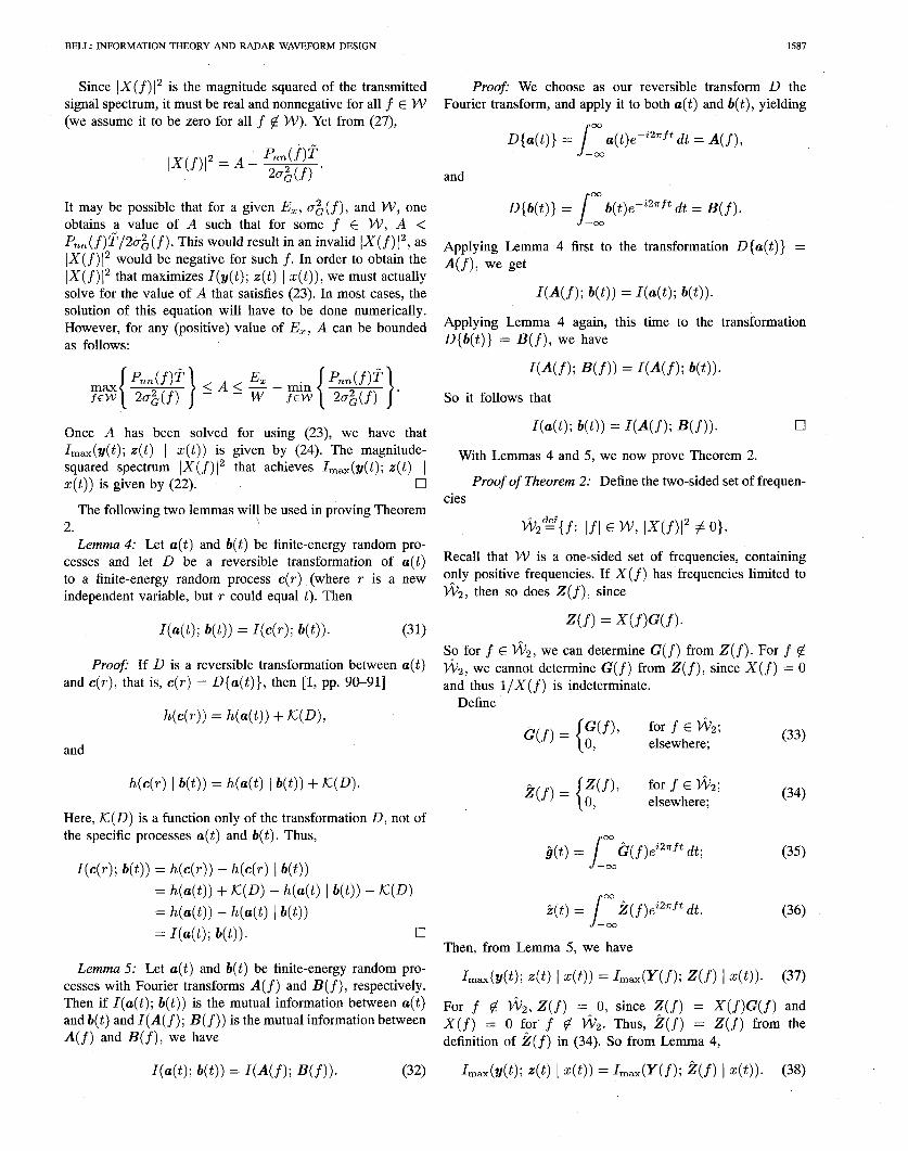
Fig. 3. (a) “Water-filling” interpretation of the magnitude-squared spectrum \X(f)[’ that maximizes the mutual information I(y(t); g(t) 1 z(t)). (b) Magnitude-squared spectrum IX(f)lz that maximizes I(y(t); g(t) 1 z(t)). Note the relationship to the shaded area in (a).

An interesting interpretation of the relationship between IX(f)/“, A, P,,(f), and g:(f) is shown in Fig. 3. Compar- ing (5) and Fig. 3, we see that the total energy E, corresponds to the shaded area in Fig. 3(a). The difference between the line of value A forming the upper boundary of the shaded region and the curve forming the lower boundary of the shaded region is lX(f)12. This difference is displayed in Fig. 3(b).

This interpretation of Fig. 3, called the “water-filling” interpretation, arises in many problems dealing with the spectral distribution of power and energy in information theory [21, p. 3891.

To further illustrate the behavior of lX(f)12 as a function of the target spectral variance g:(f) and the noise power spectral density, consider the example of Fig. 4. In Fig. 4(a) we have the spectral variance 0; (f) In Fig. 4(b) we have the power spectral density P,,(f). In Fig. 4(c) we have r(f) = %0)v~::(f), f t’ a unc ion of both the power spectral density P,,(f) of the noise and of the spectral variance g&(f). In Fig. 4(d) we have the resulting magnitude-squared spectrum lX(f)j2 for the waveforms z(t) that maximize I(y(t); g(t) I x(t)). Note that because of the assumed bandwidth constraint, W = [fo, fo + W ], lX(f)12 = 0 for all f $ W . In the next section, we will examine a more realistic and detailed example numerically, in order to illustrate these results more clearly.

We have assumed that the random impulse response g(t) is a Gaussian random process. As a result, the scattered signal z(t) is a Gaussian random process. The received signal y(t) is also a Gaussian random process, since the noise in the channel is additive Gaussian noise. Thus, for a given o&(f), we are solving for the mutual information in the case of an additive Gaussian noise channel with a Gaussian input. As is well’ known, in the case of the additive Gaussian noise channel, for a channel input with a given variance g2, the mutual information between the channel input and the channel output is maximized when the input is Gaussian. Then by assuming that g(t) is a Gaussian random process, we have selected a Gaussian input process for an additive Gaussian noise channel in our problem. By solving for the maximum mutual information

f

/Fig. 4. Example illustrating the resulting lX(f)j’ for a given u&(f)

:and Pnn(f). (a) Example o&(f). (b) Example P,,(f). (c) Resulting

I(f) = Pnn(.f)?/20&(f). (d) Resulting lX(.f)12.

Lnax(Y(t)~ g(t) I d t)L we have derived an upper bound on the maximum, achievable mutual information between y(t) and g(t) for any g(t) with spectral variance CJ& (f) under the imposed bandwidth and energy constraints, whether g(t) is Gaussian or not. In the case when g(t) is Gaussian, as we have assumed, this upper bound is achieved.

VI. EXAMPLES AND COMPARISONS

A. Detection Waveform Examples

We first consider an example that illustrates the use of the design procedure and shows the effect that the transmission of various waveforms with identical energy can have on the output signal-to-noise ratio. Assume that the stationary additive Gaussian noise is white, with power spectral density sm(f) = No/T and assume that the target impulse response h(t) has Fourier transform H(f) given by

H(f) = 0”: L for If1 I W for If\ > W .

Here 5 is a constant, which for convenience is taken to be m so that


TABLE I SIGNAL-TO-NOISE RATIOFOR z,(t) = ,/L5&(cuT/2, 2t/T)

n 2WT = 2.55 2WT = 5.10

0.9663, LOOOE, 0.912Ez 0.9993, 0.519E, 0.9973, O.llOE, 0.961%, O.O09E, 0.7483, O.O04E, 0.321E,

- O.O61E, - O.O06E,

This being the case, we have

Here GE = 27rIV. So the optimal 2(t) is a solution to the integral equation

J T/2 &J:,(t) = GL(WW sin 27rW(t - 7) d7

-T/2 27rW(t- T) ’

which is known [13] to have a countable number of solutions for n = 0, 1, 2,.... The solutions to this equation are known as the angular prolate spheroidal functions, and are designated 5’0~ (cxT/2, 2t/T). The associated eigenvalues X, can be written in terms of the radial prolate spheroidal functions, which are designated as RF: (aT/2, 1). The eigenvalues and their associated eigenfunctions are given by X, = 2WTRg(cxT/2 l), and sn(t) = So,(aT/2, 2t/T), for n = 0, 1, 2,. *.i

The sequence of eigenvectors X0, Xi, X2,. . . , X,, . . . is a positive decreasing sequence in n. So the largest eigenvector occurs when n = 0. Thus, the solution 2(t) with energy E, is

Z(t) = &%90&T/2, 2t/T), and its associated eigenvalue is

x - 2WTRh;‘(aT/2 1) max - , .

The signal-to-noise ratio in this case is

= 2WTE,R$,&T/2 1) > .

In order to demonstrate the effect of the wave shape of the transmitted waveform on the output signal-to-noise ratio, consider the effect of transmitting the waveforms x,(t) = GSo,(aT/2, 2t/T), for n = 0, 1, 2, ... . All of these waveforms have transmitted energy E,, but the resulting signal-to-noise ratios are X,E,. As noted previously, {X,} is a positive decreasing sequence of n, and thus XoE, > XlE, > X2Ez > . . . . So we see that the output signal-to-noise ratio is definitely a function of the transmitted waveform. In Table I, we show the resulting signal-to-noise ratio for the cases of 2WT = 2.55 and 2WT = 5.10. (The eigenvalues were obtained from [13, p. 1941.) As we can see, the signal-to-noise ratios drop off very quickly for n > 2WT. So we see that the wave-shape or spectral content of the transmitted waveform plays a significant role in the resulting signal-to-noise ratio.

Physically, we can interpret these results by noting that the maximum signal-to-noise ratio occurs when the target mode with the largest eigenvalue is excited by the transmitted waveformIn order to obtain the largest response possible from the target, we put as much of the transmitted energy as is possible into exciting this mode. This maximizes the signal-to- noise ratio and thus provides the best possible target detection performance under the imposed constraints.

Table I shows that it is possible to have more than one waveform with almost maximum response. For example, in the case where 2WT = 5.10, the waveforms corresponding to n = 1, 2, 3 give an output signal-to-noise ratio almost as large as the optimal waveform (n = 0). In fact, the n = 3 waveform produces a signal-to-noise ratio only 0.18 dB below that of the optimal waveform. Thus, not only can any one of these four waveforms be used with a resulting output signal-to-noise ratio comparable to the optimal, but any linear combination of these four waveforms can be used as well, yielding a family of waveforms with nearly optimal detection properties.

We now consider the problem of designing a waveformlre- ceiver-filter pair that is optimal for detecting a perfectly conducting metal sphere of radius a in the presence of stationary white noise. We will compare the output signal-to-noise ratio of the resulting waveform to that of a pulse-modulated sinusoid and compare their target detection capabilities.

In order to apply the waveform/receiver-filter pair design procedure to a perfectly conducting sphere of radius a, we must find its impulse response h(t). We assume a monostatic radar system with identical linear transmit and receive antenna polarizations. Thus, we are interested in the backscatter impulse response. The backscatter impulse response of a perfectly conducting sphere, when both transmit and receive antennas have identical linear polarization, has been calculated by Ken- naugh and Moffatt, using the physical optics approximation [22]. The physical optics approximation is used here in order to simplify the calculation of h(t) and provide an analytically tractable solution. The physical optics approximation to the impulse response accurately predicts high frequency scattering behavior and corresponds to the early-time component of the target impulse response, which for many real targets contains most of the total scattered energy [23]. For the mathematical basis of the more general treatment, see [24].

This impulse response can be written as

h(t) = -:6(t) + i[u(t) - u(t - 2a/c)].

Here, a is the radius of the sphere, c is the velocity of light, 6(t) is the Dirac delta function, and u(t) is the unit step function, defined as

for t > 0; for t < 0.

Applying the waveform/receiver-filter design procedure of Theorem 1, we must first calculate the Fourier transform of h(t). Doing so, we find that

H(f) = -& + Ge--i27rfa si;;;;; ) [ 1 (44)


Fig. 5. Magnitude-squared spectrum jH(f)1’ versus f.

where 6 = a/c. The magnitude-squared spectrum IH is thus

f)12

- 2(si;$p) cos2af8]. (45)

A plot of IH( appears in Fig. 5. Next, we find the inverse Fourier transform of the function

IH(f)12/%m(f)~ F or white noise, S,,(f) = NO/~. Thus, we have

- $ (“‘$3 cos 2nfh. (46)

Calculating the inverse Fourier transform of (46), we obtain L(t) as specified in step 1 of our design procedure. Define the two functions

and

Va(t) = ; - Id/a, {

for ItI 5 a; > elsewhere

for (tl 5 a; elsewhere.

Then we have

L(t) = L

O” lfw12 g27r.ft & NoI2

= g)(t) + TV& - $?“(“)

* [cqt - 6) + qt + ti)]

= g-)(t) + &v&(t) - -&B2&

Next, we solve the integral equation

s

T/2 x,,qt) = i+-)L(t - T) dr

-T/2

(47)

for an eigenfunction g(t) corresponding to the maximum eigenvalue X,,, . For L(t) as given in (47), we must solve

= + TV& - $3-&t) 1 g(t) dT 262 T/2 ZZ- J No -T/2

6(t - T)?(T) dr

+ $--;,;[I&(t - T) - Bzs(t - T)]?(T) d,r. (48)

From (48), we see that if i(t) is an eigenfunction corresponding to the maximum eigenvalue A,,,, it must also be an eigenvector of the integral equation

n CLrn&qq = A No~~,~[v,i(t~)-n,,(t-,)].E(T)d~ (49)

corresponding to the maximum eigenvalue pL,,,. Note that x max = 222/No + ~Umax.

For convenience in our analysis, we will assume that 2(t) has unit energy (i.e., E, = 1). In addition, for computational convenience, we assume a normalized value of 6 = 1. Although such a value of 6 does not correspond to values typically encountered in practice, these results can be applied to more typical values by scaling both the amplitude of the received signal and the time axis linearly in the length unit.

Solving the integral of equation (49) numerically for T = 1, 25, 50, 100, 250, and 500, we obtain the eigenvalues pmax of (49) and thus the eigenvalues X,,, of (48), allowing us to determine the resulting signal-to-noise ratio in each of these cases.

For the purpose of comparison with more typical radar waveforms, we will consider the response of the target to a pulse modulated sinusoid of duration T with unit energy. The receiver-filter will be a matched filter matched to the transmitted waveform-the form of receiver-filter normally used in radar detection problems.

Such a waveform can be expressed as

x(t) = P&,2(t) cos 2rf& (50)

Here, for fixed T, p is a normalizing constant such that the waveform has unit energy.

In order to obtain the most favorable result when transmitting a waveform as specified in (50), we must select the carrier frequency in order to take advantage of the resonance of the spherical scatterer as expressed by I H(f)j2. From Fig. 5, we see that IH( h as its peak value at a frequency between 0.25/G and 0.5/G. It was determined numerically that IH( takes on a maximum value of 1.5862h2 at a frequency of f = 0.325116.

Let X(f) be the Fourier transform of the transmitted waveform x(t) as given in (50). Then the matched filter matched to this waveform that gives the maximum signal- to-noise ratio at time to is specified by the transfer function

-. R(f) = JGX(f)e--a2.rrfto

Snn(f) ’ (51)

IEEE TRANSACTIONS ON INFORMATION THEORY, VOL. 39, NO. 5, SEPTEMBER 1993

TABLE II SIGNAL-M-NOISE RATIOS MULTIPLIED BY No FOR PULSED SINUSOID

AND OPTIMAL DETECTION WAVEFORMS FOR VARIOUS T

T Pulsed Optimal Improvement Sinmnid

1 1.1454 2.1737 2.78 dB 25 2.7917 3.9108 1.46 dB 50 2.8183 3.8682 1.38 dB 100 2.8354 3.7477 1.21 dB 250 2.8615 3.7464 1.17 dB 500 2.8645 3.4967 0.87 dB

where k is any nonzero constant. The signal-to-noise ratio at time to is given by

S ( > F to= =

For white noise with power spectral density Snn(f) = No/2 and R(f) as given in (51), noting that H(f) is a conjugate- symmetric function of f, this simplifies to

From (44), we have that when & = 1 as in our example,

cos27rf - 1. (53)

For x(t) as given in (50), X(f) is given by

X(f) = ex 2

sin ~(f - fo)T + sin r(f + fo)T df - fo)T df+ fo)T 1 ’

and ]X(f)12 is given by

Using (52), (53), and (54), we can solve for the signal-to- noise ratio that results when x(t) is the unit energy pulsed sinusoid given in (50). This is done for T = 1, 25, 50, 100, 250, and 500. The values of @ that provides a unit-energy waveform for each of these T are calculated numerically. Table II shows the resulting signal-to-noise ratio for these unit-energy pulsed sinusoids with their associated matched filters as well as the signal-to-noise ratio that results when an optimal waveform/receiver-filter pair is matched to the sphere being detected. In addition, we note the improvement (in decibels) in the output signal-to-noise ratio for the optimal waveform/receiver-filter pair over the pulsed sinusoid and its associated matched filter.

There is a significant improvement in the resulting signal- to-noise ratio when the optimal waveform/receiver-filter pair is used over that which occurs when a more typical ad hoc procedure is used. This is shown in Table II. For the range of T examined, the optimal waveform/receiver-filter pair provides approximately 1.2-2.8 dB of gain over the pulsed sinusoid with its associated matched filter. Considering that the received power is inversely proportional to the range to the fourth power, such gains would correspond to an increased detection range of 7-17%. In typical aircraft detection radar systems where the target is assumed to be a point target, the gain could be even greater, since the carrier frequency of the pulsed sinusoid would not be specifically selected to match the resonance of the sphere. Thus, in radar target detection problems where knowledge of the target impulse response is known a priori, a significant gain in detection signal-to-noise ratio can be achieved using the waveform/receiver-filter design procedure described in Theorem 1.

B. Estimation Waveform Examples

We now consider an example illustrating Theorem 2 and the results of Section V. In doing so, we will examine the characteristics of the optimal transmitted signal’s spectrum and the amount of information obtained.

We will assume that a radar system is observing a target at a range of 10 km. We will assume that the radar is a monostatic radar with an antenna having an effective area A, = 3 m2, an RF bandwidth of 10 MHz, a transmitter frequency centered at 1 GHz, and we will assume that the antenna is pointed directly at the target under observation. This gives us a frequency interval W of

W = [fo, f. + W ] = [0.995 GHz, 1.005 GHz].

We will consider this radar system with average power constraints ranging from 1 W to 1000 W and observation times ranging from 10 ~LS to 100 ms.

We assume that the target under observation has a finite- energy, Gaussian impulse response g(t) with spectral variance u&(f) given by

&f> = Bexp {-4f - .fpj21.

Here, B and Q are constants that respectively characterize the magnitude of the spectral variance a&(f) and the rate at which it decreases as If - f, ] increases.

We will assume in our example that

c&J = lo-13.g ,

a value illustrating well the effect of the transmitted waveform’s spectral characteristics for the 10 MHz system bandwidth being considered. We will use a value of B which results in a spectral variance &(f,) that corresponds to a variation of 1 m2 in the target radar cross section at a frequency of fP = 1 GHz. This value is

B = 7.9577 x 10-16.

We will assume that the additive Gaussian noise present at the radar receiver is thermal noise that is white over the


LYflr 2 T 2.0 x IO-‘J-s

aI T

4.0 x lo-‘J-s

0.996 0.996 0.998 1.000 0.998 1.000 1.002 1.004 1.002 1.004

Fig. 6. r(f) = Pnn(f)T/2a&(f) as a function of f. Fig. 8. jX(f)12 for T = 10 ms and P, = 100 W.

lxfjJ12 12.0 x 1O-7 J-s

, : ; : : :“::;I; : ii_ 0.996 0.998 1.ooo 1.002 1.004 ’

Fig. 7. /X(f)/’ for T = 10 ms and P, = 1000 W.

frequency interval W and that its effective noise temperature is T, = 300 K. Hence, the resulting one-sided noise power spectral density is [26, p. 291

Pnn(f) = No = ICT, = (1.381 x 10-23J/K)(300 K) - 4 1430 x 1O-21 J. - .

Here, k = 1.381 x 1O-23 J/K is Boltzmann’s constant. By definition, r(f) is given by

For ? = T = 10 ms, this becomes

r(f) = (2.7835 x lop85 - s) exp [a(f - f,)“].

A plot of this r(f) is shown in Fig. 6. For p = T = 10 ms, we consider the two cases of

P, = 1000 W and P, = 100 W . In both cases we must solve

E, = P,T = .I

max P, A - df)ld W

with respect to A and then find ]X(f)12 = max [0, A -<r(f)]. Recall that this formula gives ]X(f)12 for positive frequencies only, but that IX(f) ] 2 is an even function, so ]X(f)12 = ]X(-f)12 for f < 0. Plots of ]X(f)12 for positive f in the cases of P, = 1000 W and P, = 100 W are given in Figs. 7 and 8, respectively. From (24), the mutual information I(y(t); g(t) ] z(t)) is given by the integral

1(y(~); g(t) 1 x(t)) =.‘J’ max [0, In A - lnr(f)] df. W

10 100 Average Power Px , Watts

I 1000

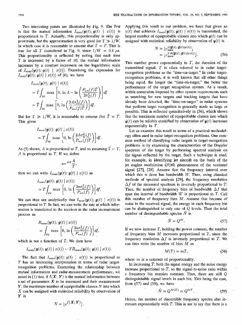
Fig. 9. I,,,(y(t); g(t) 1 s(t)) as a function of T and P,.

For P, = 1000 W and P, = 100 W , the resulting values of I(Y(Q g(t) I d t)) are 2.3815 x lo5 nats and 2.2152 x lo5 nats, respectively.

In the case of P, = 100 W , fi c W is given by

So, in this case,

[0.995698 GHz, 1.004302 GHz]. (55)

only 8.604 MHz of the available 10 MHz of RF bandwidth should be used by the radar system. This is because more information is obtained by concentrating the energy in 6 and providing a greater signal-to-noise ratio in W than by distributing the energy across W . The latter would provide a greater number of degrees of freedom to be measured, but they would be measured less reliably. The ]X(f)12 of (55) optimizes this tradeoff between the measured number of degrees of freedom in the measurement and the reliability of the individual degrees of freedom in the measurement-the optimization being done so as to maximize the mutual information I(y(t); g(t) ] Z(t)).

We will now display the results of the numerical solution of (23) and (24) for the mutual information I(y(t); g(t) ( x(t)) as a function of both T and the average available power P,. This numerical solution was carried out for values of T equal to 10 ps, 100 ps, 1 ms, 10 ms, and 100 ms. For each of these values, the average power P, varies over the range of from 1 W to 1000 W . All integrations were numerically carried out using the Gaussian Quadrature Method [25, pp. 322-3261. The resulting maximum values of I(y(t); g(t) ] x(t)) are plotted in Fig. 9.


Two interesting points are illustrated by Fig. 9. The first is that the mutual information lmax(y(t); g(t) 1 z(t)) is proportional to T. Actually, this proportionality is only approximate, but the approximation is very good for T > l/W , in which case it is reasonable to assume that ? = T. This is true for all T considered in Fig. 9, since l/W = 0.1 pus. This proportionality is reflected by noting that each time T is increased by a factor of 10, the mutual information increases by a constant increment on the logarithmic scale of l;niLx(y(t); g(t) ] z(t)). Examining the expression for L&Y(~); g(t) I x:(t)) of (61, we have

But for T > l/W , it is reasonable to assume that p = T. This gives

As (5) shows, A is proportional to T, and so assuming F = T, A is proportional to T. If we define

.=d.f$;

then we can write Imax(y(t); g(t) I z(t)) as

Lnax(Y(t); g(t) I dt>)

We can thus see analytically that ImiLx(y(t); g(t) 1 z(t)) is proportional to T. In fact, we can write the rate at which information is transferred to the receiver in the radar measurement process as

anax(Y(t); g(t) I z(t))

which is not a function of T. We then have

L&Y(~); g(t) I 441 = TKnax(~(t); g(t) I x:(t)). The fact that I max(y(t); g(t) 1 z(t)) is proportional to

T has an interesting interpretation in terms of radar target- recognition problems. Examining the relationship between mutual information and radar-measurement performance, we noted in (1) that, if 1(X; Y) is the mutual information between a set of parameters X to be measured and their measurement Y, the maximum number of equiprobable classes N into which X can be assigned with statistical reliability by observation of Y is

Applying this result to our problem, we have that given an z(t) that achieves Imax(y(t); g(t) ( z(t)) is transmitted, the largest number of equiprobable classes into which g(t) can be assigned with statistical reliability by observation of y(t) is

N = Lax ~(Yw/wl4tq

= max ~~TR(Y(t);g(t)ll(t))]. (56)

This number grows exponentially in T, the duration of the transmitted signal. T is often referred to in radar target- recognition problems as the “time-on-target.” In radar target- recognition problems, it is well known that all other things being equal, the longer the “time-on-target,” the better the performance of the target recognition system. As a result, within constraints imposed by other system requirements such as searching for new targets and tracking targets that have already been detected, the “time-on-target” in radar systems that perform target recognition is generally made as large as possible. This is reflected quantitatively in (56), which shows that the maximum number of equiprobable classes into which g(t) can be reliably classified by observation of y(t) increases exponentially in T.

Let us examine this result in terms of a practical methodol- ogy often used in radar target-recognition problems. One common method of classifying radar targets in target-recognition problems is by examining the characteristics of the Doppler spectrum of the target by performing spectral analysis on the signal reflected by the target. Such a technique is used, for example, in identifying jet aircraft on the basis of the jet engine modulation (JEM) phenomenon of the scattered signal ]27], [28]. Assume that the frequency interval over which this is done has bandwidth W . Then, ‘using classical methods of spectral analysis [29], the frequency resolution Af of the measured spectrum is inversely proportional to T. Thus, the number of frequency bins of bandwidth Af that span the interval of bandwidth W is proportional to T. Call this number of frequency bins M. Assume that because of noise in the received signal, the energy in each frequency bin can be distinguished to only one of Q levels. Then the total number of distinguishable spectra fi is

#=Q”. (57)

If we now increase T, holding the power constant, the number of frequency bins M increases proportional to T, since the frequency resolution Af is inversely proportional to T. We can thus write the number of bins M as

M(T) = mT, (58)

where m is a constant of proportionality. In increasing T, both the signal energy and the noise energy

increase proportional to T, so the signal-to-noise ratio within a frequency bin remains constant. Thus, there are still Q distinguishable signal levels in each bin. This being the case, from (57) and (58), we have

j(j = QM(T) = Q"T. (59)

Hence, the number of discernible frequency spectra also increases exponentially with T. This is not to say that there is a


direct equivalence between the discernible frequency spectra and the equiprobable classes of g(t) to which (56) refers, but this heuristic example does show that the concept of the number of classes into which a target recognition system can classify targets increasing exponentially with “time-on-target” is not foreign to radar target-recognition problems. So the behavior of (56) is intuitively satisfying.

It is important to note that when a waveform x(t) that achieves r,,,(y(t);g(t) 1 x(t)) is transmitted, the N equiprobable classes referred to in (56) are not under the control of the radar but are a function of the target ensemble. Actually, (56) states that the probability space R can be partitioned into N subsets Rr , 02, + . . , a~, where

Pr{L&-&}=$ for Ic = l,..s,N,

where N is given by (56). These N subsets 01, 02, . . . , QN, which form a partition of fi, correspond to a set of N classes into which g(t) can be reliably classified by observation of g(t). These N classes may not, however, correspond to classes that are of interest to the user of the radar system. Generally, the user will have knowledge of x(t) and will wish to classify the radar target into one of V classes d1, d2, . . . , dv based on observation of y(t).

These classes may be linked to the physics of the problem, such as the case where the classes dk describe relative target size, or the classes may be less connected with the physics of the problem, such as in the case where only two target classes A1 and dz are of interest: whether the aircraft being observed is friendly or hostile. In general, the problem of assigning a target to one of the classes in A = {Al, Aa, . . . , dv} based on observation of y(t) can be viewed indirectly as finding a mapping from C: R --f d, such that for k = 1,. 1. , N, each Qk is mapped to one of the dj with a reasonable probability of error in determining the proper target class. As N becomes larger and the partition of R becomes finer, we would expect the performance of the best mapping C to improve for fixed V. Because N is an exponentially increasing function of I(y(t); g(t) I4t)L we would expect the probability of correct classification into one of the classes in A to improve as I(y(t); g(t) ( z(t)) becomes larger.

Returning again to the results in Fig. 9, we note the second important point it conveys: in our example, a very large amount of information is contained in the radar measurements. For example, for T = 100 ps and P, = lOW, I(y(t); g(t) 1 x(t)) is approximately 100 nats, which equals approximately 144 bits. The corresponding N calculated from (56) to 2.69 x

1043. Thus, we can conclude that a significant amount of information can be obtained about the target in the radar measurement process. In order to put this information to use, signal processing algorithms must be developed. The form these take will generally be highly dependent on the specific purpose for which the radar measurements will be used.

C. Comparison of Detection and Estimation Waveforms

We now compare the characteristics of the optimal detection and estimation waveforms. This will be done by considering their magnitude squared spectra lx(f)]‘. If we interpret

/H(f) I2 as “target response” in the detection waveform design problem and g;(j) as “target response” in the estimation waveform design problem, we see that lX(f)12 tends to get larger at frequencies in which the “target response” gets larger, and smaller at those frequencies at which the power spectral density of the noise gets larger. As T becomes large such that L(t) in Theorem 1 is approximately 0 for It 1 > T/2, we have

for the optimal detection waveforms, where a is a constant. In the case of optimal estimation waveforms, from (4), using the two-sided power spectral density Snn(f) = Pnn( Ifl)/2, we have

lX(f)12 = max 0, A - &m(f)+ 1 4$(f) .

The power spectral density of the noise enters into the two solutions in two quite different ways. Hence the form of the magnitude-squared spectrum of the two waveforms is quite different. While the waveform design for optimal target detection put as much energy as possible into the mode of the target that gave the largest response when weighted with respect to the noise, the waveform design for optimal estimation distributes the available energy in order to maximize the information obtained about the target. This is in agreement with the intuitive idea that lead to the investigation of the information extraction capabilities of radar waveforms in the first place. Because the optimal detection waveforms given by Theorem 1 concentrate on placing as much energy as possible into the largest scattering mode under the imposed waveform duration constraints, they ignore the smaller scattering modes. It is possible that these smaller modes contain a significant quantity of information useful for describing the target, perhaps information useful in differentiating between two very similar targets w.hose largest scattering modes may be very similar. In Theorem 2, we have looked at how to distribute this energy to maximize the mutual information in the case where the target ensemble could be modeled as a finite-energy Gaussian target impulse response. However, even when this model does not directly apply, the results can serve as a qualitative guide to the proper distribution of energy among target scattering modes for target detection and information extraction radar waveforms.

VII. SUMMARY

We have shown that in the case of extended radar targets, the resonance phenomenon that occurs when the transmitted radar waveform is scattered by the target can be exploited to provide a larger signal-to-noise ratio at the output of the radar receiver than would result if we simply used an arbitrary waveform x(t) of energy E, with a receiver-filter matched to z(t) and the noise environment.

Physically, we can interpret -this result by noting that the maximum signal-to-noise ratio occurs when the mode of the target with the largest eigenvalue is excited by the transmitted waveform. In order to obtain the largest response possible


from the target, we put as much of the transmitted energy as is possible into exciting this mode. This gives us the largest possible signal-to-noise ratio and thus the best possible target detection performance under the imposed constraints. We note however that other scattering modes of the target may be useful for identifying or characterizing the target, so putting as much energy as possible into the mode with the largest eigenvalue will not generally be the best method of obtaining the maximum amount of information useful in describing the target. When our task is target identification or information extraction, we may thus wish to distribute the transmitted energy among the different target modes in a different manner. Theorem 2 describes how to distribute the energy in such a way that the mutual information between the target ensemble and the received waveform is maximized. As we saw in Section II-C, the greater this mutual information, the better we would expect the radar’s classification and estimation capabilities to be.

The direct application of the results in Theorem 1 arise in radar problems where one is attempting to detect the presence of a target when one has a priori knowledge of its scattering characteristics-that knowledge being represented by the target impulse response h(t). Such a situation might arise if we are trying to detect a high priority target providing a very small radar return. In such a situation, the additional received energy obtained by taking advantage of the target’s resonant behavior may provide a significant improvement in detection performance.

As a practical matter, the optimal waveform solutions may not be easy to implement in real radar systems, since for reasons of power efficiency, these systems often operate with transmitter amplifiers in saturation. Because saturated amplifiers typically require that the waveform have (approximately) constant envelope, many of the optimal solutions obtained using the waveform/receiver-filter pair design procedure of Section VI-A cannot be used in radar systems that operate with a saturated transmitter. Still, the basic idea of putting as much of the energy as possible into the target’s largest scattering mode under the design constraints on the waveform (which might be expanded to include a constant envelope constraint) is useful to keep in mind. In particular, the pulsed sinusoid used for comparison in Section III-A had its carrier frequency selected to give the largest possible response from the sphere. The selection of fu in this example is clearly better then ignoring the target resonance phenomenon and arbitrarily selecting the carrier frequency.

Finally, note that the shape of a radar signal, and not just its energy alone, can have a significant effect on extended target detection performance. This fact is often overlooked in the radar engineering community, largely as a result of the fact that when one uses a matched filter to detect a waveform in stationary additive noise, detection performance does not depend on the shape of the waveform being detected-as long as the receiver-filter being used is matched to the waveform to be detected and the additive noise’s power spectral density. As a result, if we are considering a point target, then h(t) = &(t - to), and the shape of the transmitted waveform would have no effect on the output signal-to-noise ratio. However, as we have seen in Section IV, this is not true of extended targets,

where h(t) # aS(t - to). It is advantageous to keep this fact in mind when considering extended targets and not extrapolate the point-target results to the extended target case, as is often done. For a point target, the waveform/receiver-filter design procedure produces a solution where x(t) is any arbitrary waveform x(t) with energy E, and r(t) is its associated matched filter.

In the case of the design of a waveform z$t) that optimizes the detection of a target of known impulse response h(t), we noted that the solution corresponds to an eigenfunction with energy E, corresponding to the largest eigenvalue of the integral equation of (22). We noted that these results could be interpreted, in the case of additive white Gaussian noise, as putting as much of the transmitted energy as possible into the largest mode of the target under the time and bandwidth constraints on the transmitted waveform. The result was that we obtained the largest possible signal-to-noise ratio, and thus the optimal detection performance, under the constraints on the transmitted waveform. We also noted, however, that the other eigenfunctions, corresponding to different modes of the target, could contain significant information about the target. So if we wished to extract information about the target, it might be advantageous to distribute the available energy among the various modes. This illustrates that optimal waveforms for detection and estimation of extended radar targets can be very different in nature. Viewing the characteristics of these waveforms in terms of the distribution of energy among target scatttering modes gives both physical and information- theoretic insights into the design and performance of these waveforms. As the technology for adaptive waveform radars becomes more widespread, these insights should be valuable in effectively utilizing this technology.

ACKNOWLEDGMENT

I would like to thank Prof. E. C. Posner of the California Institute of Technology and an anonymous reviewer for their comments and suggestions on improving the presentation of this material.

111

121

131

[41

[51

161

171

Is1

REFERENCES

C. E. Shannon, “A mathematical theory of communication,” Bell Syst. Tech. J., vol. 27, pp. 379-423 and 623-656, 1948; reprinted in C. E. Shannon and W. W. Weaver, The Mathematical Theory of Communica- tion. Urbana, IL: University of Illinois Press, 1949. P.M. Woodward and I. L. Davies, “A theory of radar information,” Phil. Msg., vol. 41, pp. 1101-1117, Oct. 1951. P.M. Woodward, “Information theory and the design of radar receivers,” Proc. IRE, vol. 39, pp. 1521-1524, Dec. 1951. P.M. Woodward and I.L. Davies, “Information theory and inverse probability in telecommunications,” Proc. IEE, vol. 99, Part III, pp. 37-44, Mar. 1952. I. L. Davies, “On determining the presence of signals in noise,” Proc. ZEE, vol. 99, Part III, pp. 45-51, Mar. 1952. - P.M. Woodward, Probability and Information Theory with Applications to Radar. London, England: Pergamon, 1953. V. S. Frost and K. S. Shanmugan, “The information content of synthetic aperture radar images of terrain,” IEEE Trans. Aerospace Electron. Syst., vol. AES-19, no. 5, pp. 768-774, Sept. 1983. C. H. Wilcox, “The synthesis problem for radar ambiguity functions,” Math. Res. Center, U.S. Army, Univ. Wisconsin, Madison, WI, MRC Tech. Summary Rep. 157, Apr. 1960; reprinted in R. E. Blahut, W. M. Miller, and C. H. Wilcox, Radar and Sonar, Part I. New York: Springer-Verlag, 1991.


[91

[lOI

1111

W I

P31

P41

P51

1161

P71

PI

H. Naparst, “Dense target signal processing,” IEEE Trans. Inform. Theory, vol. IT-37, no. 2, pp. 317-327, Mar. 1991. S. Ramo, J.R. Whinnery, and T. Van Duzer, Fields and Waves in Communicat ions Electronics, 2nd ed. New York: Wiley, 1984. D. 0. North, “An analysis of the factors which determine signal-noise discrimination in pulsed carrier systems,” RCA Lab., Rep. PTR-6C, reprinted in Proc. IEEE, vol. 51, pp. 1016-1027, July 1963. R.N. Bracewell, The Fourier Transform and Its Applications. New York: McGraw-Hill, 1986. H. L. Van Trees, Detection, Estimation, and Modulation Theory, Part 1. New York: Wiley, 1968. C. W . Helstrom, Statistical Theory of Signal Detection. New York: Pergamon, 1968. T. Berger, Rate Distortion Theory. Englewood Cliffs, NJ: Prentice- Hall, 1971. F. Kanaya and K. Nakagawa, “On the practical implication of mutual information for statistical decision making,” IEEE Trans. Inform. Theory, vol. 37, no. 4, pp. 1151-1156, July 1991. M. R. Bell, “Information theory and radar: Mutual information and the design and analysis of radar waveforms and systems,” Ph.D. dissertation, California Inst. Technol., Pasadena, 1988. A. Papoulis, Probability, Random Variables, and Stochastic Processes. New York: McGraw-Hill, 1965.

P91

W I

PI

PI

(231

v41

~51

P61

~71 PI

v91

F. B. Hildebrand, Advanced Calculus for Applications, 2nd ed. Engle- wood Cliffs, NJ: Prentice-Hall, 1976. R. J. McEliece, The Theory of Information and Coding. Reading, MA: Addison-Wesley, 1977. R. G. Gallager, Information Theory and Reliable Communication. New York: Wiley, 1968. E. M. Kennaugh and D. L. Moffatt, “Transient and impulse response approximations,” Proc. IEEE, vol. 51, no. 8, pp. 893-901, Aug. 1965. M. L. Van Blaricum, “A view of the early-time component in impulsive scattering,” in Ultra- Wideband Radar: Proc. First Los Alamos Symp., B. Noel, Ed. Boca Raton, FL: CRC Press, 1991, pp. 191-202. C.H. Wilcox, “Sonar and radar echo structure,” in Radar and Sonar, Part I, R. E. Blahut, W . M. Miller, and C. H. Wilcox, New York: Springer-Verlag, 1991. R. W . Hamming, Numerical Methods for Scientists and Engineers, 2nd ed. New York: Dover, 1973. J. R. Pierce and E. C. Posner, Introduction to Communication Science and Systems. New York: Plenum, 1980. M. I. Skolnik, Radar Handbook. New York: McGraw-Hill, 1970. M. R. Bell and R. A. Grubbs, “Modeling of jet engine modulated radar signal returns for target identification,” IEEE Trans. Aerospace Electron. Syst., vol. 28, no. 1, Jan. 1993. R. B. Blackman and J. W . Tukey, The Measurement of Power Spectra. New York: Dover, 1958.

information theory and radar waveform designmrb/resources/selpubsf/itradarwaveforms.pdfdetection of...

Documents