Imaging Microwave and DC Magnetic Fieldsin a Vapor-Cell Rb Atomic ClockChristoph Affolderbach, Member, IEEE, Guan-Xiang Du, Thejesh Bandi,

Andrew Horsley, Philipp Treutlein, and Gaetano Mileti

Abstract— We report on the experimental measurement ofthe dc and microwave magnetic field distributions inside arecently developed compact magnetron-type microwave cavitymounted inside the physics package of a high-performancevapor-cell atomic frequency standard. Images of the microwavefield distribution with sub-100-µm lateral spatial resolution areobtained by pulsed optical-microwave Rabi measurements, usingthe Rb atoms inside the cell as field probes and detecting witha CCD camera. Asymmetries observed in the microwave fieldimages can be attributed to the precise practical realization of thecavity and the Rb vapor cell. Similar spatially resolved images ofthe dc magnetic field distribution are obtained by Ramsey-typemeasurements. The T2 relaxation time in the Rb vapor cell isfound to be position dependent and correlates with the gradientof the dc magnetic field. The presented method is highly usefulfor experimental in situ characterization of dc magnetic fieldsand resonant microwave structures, for atomic clocks or otheratom-based sensors and instrumentation.

Index Terms— Atomic clocks, diode lasers, microwavemeasurements, microwave resonators, microwave spectroscopy,optical pumping.

I. INTRODUCTION

COMPACT vapor-cell atomic frequency standards(atomic clocks) [1], [2] are today widely used in

applications such as telecommunication networks [3] orsatellite navigation systems [4], and are also of interest forother scientific or industrial applications. In view of the futuredemand for highly compact but nevertheless high-performancevapor-cell clocks in these fields, laboratory clocks with state-of-the-art fractional clock frequency stabilities of 1.4 × 10−13

at an integration time of τ = 1 s [5] and down to few 10−15

Manuscript received February 3, 2015; revised April 28, 2015; acceptedMay 14, 2015. Date of publication June 30, 2015; date of current ver-sion November 6, 2015. This work was supported in part by the SwissNational Science Foundation under Grant 149901, Grant 140712, and Grant140681, and in part by the European Metrology Research Programme underProject IND55-Mclocks. The EMRP is jointly supported by the EMRPparticipating countries within EURAMET and the European Union. TheAssociate Editor coordinating the review process was Dr. Sergey Kharkovsky.

C. Affolderbach and G. Mileti are with the Laboratoire Temps-Fréquence,Institut de Physique, University of Neuchâtel, Neuchâtel 2000, Switzerland(e-mail: christoph.affolderbach@unine.ch; gaetano.mileti@unine.ch).

G.-X. Du, A. Horsley, and P. Treutlein are with the DepartementPhysik, University of Basel, Basel 4056, Switzerland (e-mail:philipp.treutlein@unibas.ch).

T. Bandi is with the Laboratoire Temps-Fréquence, Institut de Physique,Université de Neuchâtel, Neuchâtel 2000, Switzerland, and also withthe Quantum Sciences and Technology Group, Jet Propulsion Laboratory,California Institute of Technology, Pasadena, CA 91109 USA.

Color versions of one or more of the figures in this paper are availableonline at http://ieeexplore.ieee.org.

Digital Object Identifier 10.1109/TIM.2015.2444261

for τ = 104 s [6] have been reported recently. A preciseknowledge of the microwave and dc magnetic fielddistributions in such clocks is a key requirement for theirdevelopment.

In a Rb vapor-cell atomic clock, the frequency of a quartzoscillator is stabilized to the frequency of the so-calledmicrowave hyperfine clock transition |F = 1, m F = 0〉 ↔|F = 2, mF = 0〉 in the 5S1/2 ground state of 87Rb (at νRb =6 834 682 610.904 312 Hz [7] [see Fig. 2(c)]), generallydetected using the optical-microwave double-resonance (DR)scheme. In Rb clocks based on the continuous-wave (CW)DR interrogation scheme [2], [5] a ground-state polarizationis created by optical pumping [8] with a Rb lamp or laser,and the clock transition frequency is detected via a changein light intensity transmitted through the cell. In this scheme,the optical and microwave fields are applied simultaneouslyand continuously, which can cause perturbations of the clockfrequency due to the light shift effect [5], [9]. In the pulsedinteraction scheme [6], first a resonant laser pump pulsecreates the ground-state polarization, followed by two time-separated microwave pulses in the Ramsey scheme [10]. Theatomic response is then read out by a laser detection pulse.With the optical and microwave interaction separated in time,the light shift effect can be significantly reduced in thisscheme. In both approaches, the Rb atomic sample is heldin a sealed vapor cell usually also containing a buffer gas toavoid Rb collisions with the cell walls, and the microwaveis applied to the atoms using a microwave cavity resonator,which allows realizing compact clock physics packages. Forall atomic clocks employing microwave cavity resonators toapply the microwave radiation to the atoms, the uniformityand homogeneity of the resonant microwave magnetic fieldinside the cavity is of critical importance for achieving strongclock signals: selection rules for the clock transition require amicrowave magnetic field oriented parallel to the quantizationaxis defined by the applied dc magnetic field, and the pulsedscheme in addition requires a homogeneous microwave fieldamplitude for applying π /2-pulses to all sampled atoms.

The design and study of different types of microwave res-onator cavities with well-defined field distributions have beenaddressed, e.g., for compact vapor cell atomic clocks [11] andH-MASERs [12], high-performance Rb clocks based on theCW [13], [14] or pulsed optical pumping approach [6], [15],or miniaturized Rb clocks [16], [17]. In primary atomicfountain clocks, effects such as distributed phase shifts in thecavity can become relevant [18]. The impact of the microwave

Published in IEEE Transactions on Instrumentation and Measurement 64, no 12, 3629-3637, 2015which should be used for any reference to this work 1

field distribution on Rb atomic clocks using buffer-gas andwall-coated cells has been discussed in [19], and effectslike the microwave power shift have been shown to dependon the degree of inhomogeneity of the dc magnetic field(so-called C-field) applied to the atomic sample [11], [20].For a thorough understanding of a cell clock’s perfor-mance limitations, knowledge of the precise distributionand homogeneity of both the dc and microwave magneticfields applied to the atomic vapor is therefore of crucialimportance.

In practice, it is difficult to experimentally measurethe microwave magnetic field geometry and distribution in thecavity’s final configuration, notably due to the presence of thevapor cell that prevents the placement of a field probe withinits volume, and due to the field perturbations caused by thepresence of such a probe. Most studies therefore rely ondetailed analytic and/or numerical simulations of the fielddistribution, while the experimentally accessible parametersare generally integrated over the entire cell or cavityvolume, e.g., by measuring S-parameters, resonancefrequencies, and quality factor [12], [13], [15]. Furthermore,due to the limited fabrication tolerances of glass-made vaporcells, the microwave field distribution inside the cavity willvary slightly from one cell to another, which can impact onthe atom interrogation without necessarily being detectableby the methods mentioned above.

In this paper, we exploit an imaging technique using theRb atoms in our clock’s vapor cell as local fieldprobes [21]–[23] to obtain images of the microwave fielddistribution inside the cavity on a fully assembled clockphysics package and under real operating conditions with asub-100-μm lateral spatial resolution. We also show that avariant of this imaging technique can be used to obtain imagesof the dc magnetic field (C-field) applied to the cell. Thisallows assessing eventual changes in the static magnetic fieldeven after extended clock operation time, without needing todisassemble the clock physics package.

II. EXPERIMENTAL SETUP AND METHODS

In this section, we describe the microwave cavity and clockphysics package studied, as well as the experimental setup anddetection schemes used.

A. Microwave Cavity

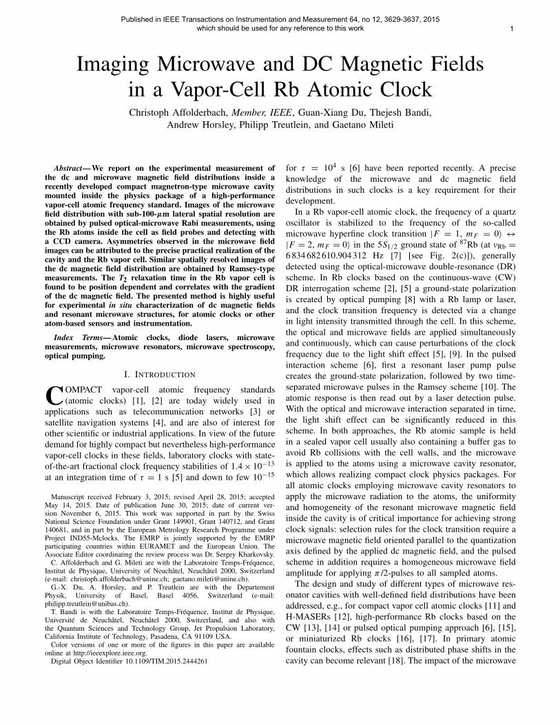
The cavity under study here has been described in detailin [5] and [13]. It is based on the loop-gap-resonatorapproach [24], also known as magnetron-type cavity [11].In our cavity, a set of six electrodes placed inside a cylindricalelectrically conducting cavity enclosure is used to create a res-onance at the precise clock transition frequency [see Fig. 1(a)].This design also imposes a TE011-like mode geometry ofthe microwave field, with the magnetic field vector essentiallyparallel to the z-axis across the Rb cell, for effectively drivingthe clock transition (magnetic dipole transition). The cavityis highly compact with an outer diameter and lengthof 40 and 35 mm, respectively, thus realizing a highly homo-geneous microwave field across the cell using a cavity with

Fig. 1. (a) Cross-sectional drawing of the microwave cavity with its electrodestructure. The coordinate system used throughout this paper is shown; thez-axis coincides with the cavity’s axis of cylindrical symmetry. (b) Assembledmicrowave cavity with the Rb vapor cell. For better visibility, the coordinatesystem is offset from its true origin here.

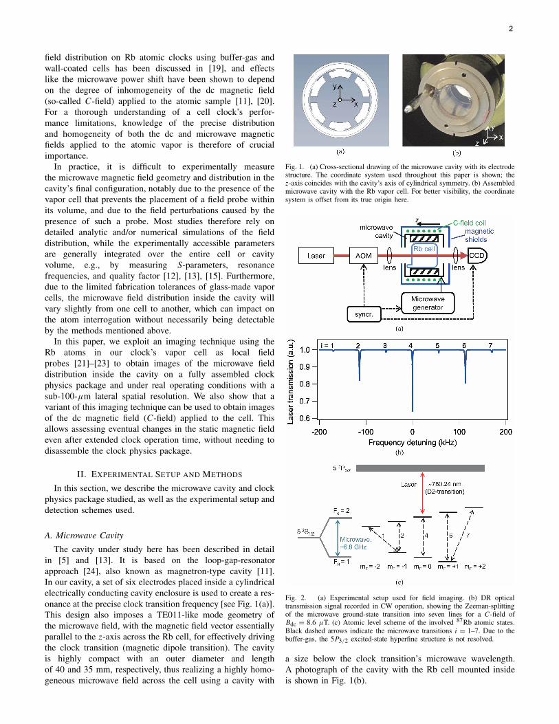
Fig. 2. (a) Experimental setup used for field imaging. (b) DR opticaltransmission signal recorded in CW operation, showing the Zeeman-splittingof the microwave ground-state transition into seven lines for a C-field ofBdc = 8.6 μT. (c) Atomic level scheme of the involved 87Rb atomic states.Black dashed arrows indicate the microwave transitions i = 1–7. Due to thebuffer-gas, the 5P3/2 excited-state hyperfine structure is not resolved.

a size below the clock transition’s microwave wavelength.A photograph of the cavity with the Rb cell mounted insideis shown in Fig. 1(b).

2

B. Clock Physics Package and Imaging Setup

For our field imaging studies, we use the modifiedRb atomic clock setup shown in Fig. 2(a). The microwavecavity (as described in Section II-A) is placed inside aclock physics package also containing a thermostat, magneticshields, and a solenoid (40-mm radius and 48-mm length)placed around the cavity for applying the dc magnetic fieldof Bdc ≈ 40 μT, oriented parallel to the z-axis. The vaporcell is made of borosilicate glass, has a diameter and lengthof 25 mm each, and is equipped with a cylindrical stem servingas Rb reservoir [see Fig. 1(b)]. It contains isotopically enriched87Rb and a 26-mbar buffer-gas mixture of N2 and Ar forsuppressed temperature sensitivity of the clock transition. Themain cell body is held at a temperature of 55 °C and the stemat 40 °C. Under these conditions, we find a mean free path ofλmf = 5 μm for the Rb atoms in the cell.

Optical pumping and detection is achieved by a laser diodewhose frequency is stabilized to the Fg = 2 → Fe = 2, 3crossover transition of the Rb D2 line, observed in an auxiliaryRb cell without buffer gas, corresponding approximately to thecenter of the collisionally broadened and shifted optical tran-sition in the buffer-gas cell [25]. The laser intensity incidentto the cavity cell was 19.7 mW/cm2 and was switched ON

and OFF using an acousto-optical modulator. The microwaveradiation was produced by a laboratory microwave synthesizerwith a frequency close to the ≈6.835-GHz clock transitionfrequency and its pulses controlled by switches. By setting themicrowave frequency to values corresponding to the differentresonances i = 1–7 shown in Fig. 2(b), the different Zee-man components of the Rb hyperfine ground-state transitionindicated in Fig. 2(c) can be selected. The typical microwavepower level injected into the cavity is around +22 dBm. Thelaser light level transmitted through the vapor cell is thenmapped onto a CCD camera or a photodiode, using imagingoptics.

C. Detection Schemes

Field imaging is performed using the method presentedin [23], based on pulsed interaction schemes using Rabimeasurements and Ramsey measurements. In both schemes,a first pump laser pulse depopulates the Fg = 2 ground-statelevel, followed by one or two microwave pulses for coherentinteraction, and finally a weak probe laser pulse reads out theresulting atomic population in the Fg = 2 state. The variationin optical density �OD of the atomic sample induced by thepulsed interaction scheme is then calculated from the laserintensities transmitted through the cell as described in [23].While in [23] imaging was performed on a microfabricatedvapor cell resulting in a spatial resolution in the z-directiondefined by a cell thickness of 2 mm, we here apply the imagingtechnique to a thick cell of 25-mm length.

Rabi measurements, using one microwave pulse of variableduration dtmw between the optical pump and probe pulses,were employed for imaging the microwave magnetic fieldamplitudes in the cavity. In this case, the microwave frequencyis tuned to the center of the selected Zeeman componentof the hyperfine transition. The observed variation in optical

density as a function of dtmw shows Rabi oscillations and isdescribed by

�O D = A − B exp

(−dtmw

τ1

)

+ C exp

(−dtmw

τ2

)sin (� dtmw + φ). (1)

Here the fit parameters are an overall constant offset A inoptical density, amplitude B of the relaxation of populationwith its related time constant τ1, and the amplitude C,time constant τ2, Rabi frequency �, and phase φ of theRabi oscillations introduced by the microwave field. By tuningthe microwave frequency to the transitions i = 1, 4, or 7, weare sensitive to the σ−, π , or σ+ component of the microwavemagnetic field, respectively, via the corresponding transition’sRabi frequency �i .

Imaging of the dc magnetic C-field was conducted usingRamsey measurements, where the microwave interaction isachieved by two π /2 microwave pulses separated by aRamsey time dtR , during which neither light nor microwave isapplied. The detected variation in optical density as a functionof dtR is described by

�O D = A − B exp

(−dt R

T1

)

+ C exp

(−dt R

T2

)sin (δ dt R + φ) . (2)

Here the fit parameters are A, B, C, T1, T2, δ, and φ, anal-ogous to (1), with T1 and T2 the population and coherencelifetimes, respectively. The Ramsey oscillation frequency δ isequal to the microwave detuning from the atomic transition.Thus, for an externally fixed microwave frequency injectedinto the cavity, the value of δ encodes the C-field amplitudeat the position of the sampled atoms, via the Zeeman shiftof the selected transition. Using the Breit–Rabi formula [26],the C-field amplitude can then be calculated from δ, andcommon-mode frequency shifts such as buffer-gas shifts canbe eliminated when combining measurements on two differenttransitions.

For construction of spatially resolved images, imagingoptics and a CCD camera are used for measuring the transmit-ted laser intensities. Using a pattern mask at the level of thecavity as well as ray transfer matrix calculation, the imagingoptics is found to result in a 1:4 demagnification of the atoms’image on the CCD sensor. In order to reduce noise and tolimit computation effort on the fitting, the CCD images werebinned into image pixels of 3 × 3 CCD-pixels. Each resultingimage pixel corresponds to a 76 μm × 76 μm cross sectionat the cell and contains the atomic signal integrated withinthis area. The imaged area has a diameter of 11 mm at thecell, and each image consists of ≈15 000 image pixels. Thetime series �OD(dtmw) or �OD(dtR) is fitted with (1) or (2),respectively, independently for each image pixel. For both (1)and (2), all the seven fit parameters are fitted independently.Examples of such fits to Rabi and Ramsey data of a typicalsingle image pixel are shown in Fig. 3, for data recorded onthe i = 7 transition. Both data sets are well described bythe fit functions of (1) and (2), respectively. Finally, the fit

3

Fig. 3. Typical examples of time-domain oscillations in the CCD signalrecorded on the i = 7 transition here. (a) Rabi data for image pixel (80, 80)from Fig. 6(c), corresponding to a microwave magnetic field amplitude ofB = 0.5 μT. (b) Ramsey data for an image pixel at the center of symmetryfrom data similar to those of Fig. 4. Insets: the pulse sequences employed.In both (a) and (b) signals are normalized such that �O D = 0 correspondsto the cell’s optical density under conditions of optical pumping but withoutany microwave interaction applied.

parameters from each pixel are recombined to obtain images ofthe physical entities of interest. Because the measurements aretaking place in the time domain, the fit parameters � and δ ofmain interest here are largely insensitive to overall variationsin the signal amplitude.

III. EXPERIMENTAL RESULTS

In the following, we discuss the images of the dc andmicrowave magnetic fields across the cell, obtained with theRabi and Ramsey interrogation schemes. Images obtainedgenerally refer to the xy plane, but certain information onthe field distribution along the z-axis can also be obtained.

A. Imaging of the DC Magnetic Field

Imaging of the dc magnetic C-field was achievedusing the Ramsey interrogation method (see Section II-C).Fig. 4 shows the C-field amplitude Bdc and T2 lifetimeimages obtained from the corresponding fit parameters of (2).Data were recorded with the microwave frequency tunedclose to the i = 2 transition and common-mode frequencyshifts were removed by using similar measurements on thei = 6 transition. The C-field amplitude is found to be very

Fig. 4. Imaging results measured on transition i = 2 (m F=1 = −1 →m F=2 = −1). Upper left panel: dc magnetic field amplitude Bdc. Lowerleft panel: T2 times. Right-hand panels: corresponding uncertainties returnedfrom the fitting routine. Left-hand panels: black crosses give the centers ofcircular symmetry found for both images. See Fig. 1 for definition of thecoordinate system used.

homogeneous, with a peak-to-peak variation of only 0.13 μT(or 0.3%) over the sampled cell region. Relative uncertaintiesreturned from the fit on each individual pixel are <0.5% forthe C-field amplitude and <8% for the T2 time. The imagesof both the C-field and T2 show a circular symmetry aroundthe same center (indicated by black crosses in the left-handpanels of Fig. 4), and do not correlate with any symme-try of the microwave magnetic field distributions measured(see Section III-B). Images of Bdc and T2 qualitativelyand quantitatively very similar to Fig. 4 are obtained whenthe microwave frequency is tuned close to the transitionsi = 1, 6, and 7. Fitting uncertainties are <1% for theC-field amplitude and on the level of 2% to 10% for T2 inall cases.

For a more quantitative analysis, we plot the C-field ampli-tude [Fig. 5(a)] and T2 [Fig. 5(b)] as functions of distance rfrom the center of symmetry (black crosses in the left-handpanels of Fig. 4), for transition i = 2. The C-field dependenceon r is well described by

Bdc(r) = C0 + C2 · r2 + C4 · r4 (3)

shown as fit in Fig. 5(a). As expected, the C-field profilesmeasured on transitions i = 1, 6, and 7 show a very similarbehavior: all the four transitions give a consistent value of Bdc(r = 0) = C0 = 40.31 μT, only slightly below the 40.41 μTcalculated from the solenoid geometry and applied current.Because the clock transition (i = 4) shifts in second order onlywith the magnetic field, determination of the C-field amplitudefrom this transition gives much bigger uncertainties, with datascatter on the level of 0.1 μT, which completely masks theC-field structure visible in Fig. 5(a).

The measured C-field amplitudes and T2 times are clearlycorrelated, as seen from Fig. 4. This can be attributed to

4

Fig. 5. (a) Radial profile of the C-field amplitude measured on transitioni = 2 (dots) and fourth-order polynomial fit to the data (solid line). (b) Radialprofile of the corresponding T2 time measured on the i = 2 transition.Solid arrows mark regions of locally higher C-field gradient and relativelylower T2 times, and dashed arrows mark regions of opposite characteristics.(c) Radial profile of the T2 time measured on the i = 4 transition.

inhomogeneous dephasing due to spatial gradients in theC-field, a process well known from nuclear magneticresonance (NMR) spectroscopy: at large r values, theRb atoms diffusing through the buffer gas sample spatialregions of more pronounced differences in C-field ampli-tude, thus resulting in reduced T2 times [27], [28]. Fig. 5(b)indeed shows a general linear decrease in T2 with r [blackdashed line in Fig. 5(b)], with a slope ∂T2/∂r = −41.6 μs/mm,which is consistent with a dependence of T2 on the fieldgradient ∂ Bdc/∂r for a C-field distribution governed by thequadratic term C2 ·r2, as is the case here. One further observesthat T2 values above (below) the linear trend are measuredin regions where ∂ Bdc/∂r is locally smaller (larger) thanthe derivative of the general polynomial of (3), marked bydashed (solid) vertical arrows in Fig. 5(a) and (b). The radialT2 profiles measured on transitions i = 1, 6, and 7 again showthe same general behavior as found for i = 2; however, resid-ual deviations from the linear trend are slightly stronger oni = 1 and 7 (recorded using the σ− and σ+ microwavemagnetic field components) than for the i = 2 and 6 case(recorded using the π microwave field component). This indi-cates a dependence of the inhomogeneous dephasing on themF quantum numbers or magnetic field component involved.

Under conditions of inhomogeneous dephasing in spin echoNMR and for linear and quadratic spatial variation of the staticmagnetic field, the overall transverse relaxation time T ∗

2 is

given by [28], [29]

T ∗−12 = T −1

2,0 + 1

3D (Gγ tR)2 = T −1

2,0 + ηG2. (4)

Here T2,0 is the T2 time at vanishing field gradient, D thediffusion constant of Rb atoms in our cell, γ the atoms’gyromagnetic factor, tR the average Ramsey time, and G thelocal gradient of the static magnetic field of relevance here. Formore complicated field distributions, numerical approaches aregenerally used [30]. The black solid line in Fig. 5(b) gives a fitof T ∗

2 (r) according to (4) to the measured distribution T2(r),using G(r) = dB(r)/dr calculated according to the fit of (3)shown in Fig. 5(a), which yields T ∗

2 (r = 0) = T2,0 =445.5(6) μs and η = 1.794(8) mm2 ·μs−1 ·μT−2 for the onlytwo free parameters of this fit. Although derived for the caseof spin echo, this curve reproduces very well the general shapeof the measured T2(r) dependence. The blue dotted curvein Fig. 5(b) gives the profile T ∗

2 (r) calculated for our cellconditions, using the same T ∗

2 (r = 0) = 445.5 μs andη = 1.2 mm2 · μs−1 · μT−2 (calculated from D = 7.1 cm2/sfor our cell conditions and tR = 0.8 ms, no free parameters).We attribute this residual difference in η to the following facts.

1) Equation (4) is derived for spin echo experiments (usingone single tR) while our measurements are obtainedusing the Ramsey scheme with varying tR .

2) The actual field gradient G(r) might be underestimatedby neglecting contributions from dB(r)/dz here.

The results still indicate that the observed variation T2(r)can indeed be caused by inhomogeneous dephasing due tomagnetic field gradients.

Fig. 5(c) shows the T2 time measured on the i = 4transition. Again, T2 shows a linear dependence on r , witha slope ∂T2/∂r = −13.3 μs/mm, approximately three timeslower than observed on i = 1, 2, 6, and 7. The mean value ofT2 = 1.5(2) ms is considerably higher than the one observedon the other transitions and is in agreement with the intrinsicclock transition linewidth measured for this cell [31].

B. Imaging of the Microwave Field

Imaging of the microwave magnetic field inside the cav-ity was performed using the Rabi interrogation scheme(see Section II-C). The microwave transitions i = 1, 4, and 7are exclusively driven by the σ−, π , and σ+ componentsof the microwave magnetic field, respectively. By tuning themicrowave frequency to each of these resonances in turn andextracting the corresponding Rabi frequencies �i from fitsof (1) to each pixel’s data, we can therefore determine theamplitude of the magnetic microwave field components as

B− = 1√3

�

μB�1

Bπ = �

μB�4

B+ = 1√3

�

μB�7 (5)

where B−, Bπ , and B+ are the amplitudes of the σ−, π ,and σ+ microwave field components, respectively [21].

5

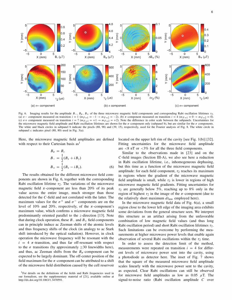
Fig. 6. Imaging results for the amplitude B−, Bπ , B+ of the three microwave magnetic field components and corresponding Rabi oscillation lifetimes τ2.(a) σ− component measured on transition i = 1 (m F=1 = −1 → m F=2 = −2). (b) π -component measured on transition i = 4 (m F=1 = 0 → m F=2 = 0).(c) σ+ component measured on transition i = 7 (m F=1 = +1 → m F=2 = +2). Note the difference in color scale between the subpanels. Uncertainties forthe microwave magnetic field amplitude and Rabi oscillation lifetimes are shown for the π -component only (subpanel b), but are similar for the σ components.The white and black circles in subpanel b indicate the pixels (88, 98) and (39, 15), respectively, used for the Fourier analysis of Fig. 8. The white circle insubpanel c indicates pixel (80, 80) used in Fig. 3(a).

Here, the microwave magnetic field amplitudes are definedwith respect to their Cartesian basis as1

Bπ = Bz

B− = 1

2(Bx + i By)

B+ = 1

2(Bx − i By). (6)

The results obtained for the different microwave field com-ponents are shown in Fig. 6, together with the correspondingRabi oscillation lifetime τ2. The variations of the microwavemagnetic field π-component are less than 20% of its peakvalue across the entire image, much stronger than thosedetected for the C-field and not correlated with the latter. Themaximum values for the σ+ and σ− components are on thelevel of 10% and 20%, respectively, of the π-component’smaximum value, which confirms a microwave magnetic fieldpredominantly oriented parallel to the z-direction [13]. Notethat during clock operation, these B− and B+ field componentscan in principle induce ac Zeeman shifts of the atomic levelsand thus frequency shifts of the clock (in analogy to ac Starkshift introduced by the optical radiation). However, in clockoperation the microwave frequency will be resonant with thei = 4 π-transition, and thus far off-resonant with respectto the σ transitions (by approximately ≥30 linewidths here),and thus, ac Zeeman shifts from the Bπ -component can beexpected to be largely dominant. The off-center position of thefield maximum for the π-component can be attributed to a shiftof the microwave field distribution caused by the cell reservoir

1For details on the definitions of the fields and Rabi frequencies used inour formalism, see the supplementary material of [21], available online athttp://dx.doi.org/10.1063/1.3470591.

located on the upper left rim of the cavity [see Fig. 1(b)] [32].Fitting uncertainties for the microwave field amplitudeare <8 nT or <3% for all the three field components.

Similar to the observations made in [23] and on theC-field images (Section III-A), we also see here a reductionin Rabi oscillation lifetime, i.e., inhomogeneous dephasing,but this time as a function of the microwave magnetic fieldamplitude: for each field component, τ2 reaches its maximumin regions where the gradient of the microwave magneticfield amplitude is small, while τ2 is lower in regions of highmicrowave magnetic field gradients. Fitting uncertainties forτ2 are generally below 5%, reaching up to 8% only in theregion of highest τ2 in the image of the π-component (due tothe relatively short maximum dtmw employed here).

In the microwave magnetic field data of Fig. 6(a), a smallregion close to the lower left edge of the imaging area exhibitssome deviations from the general structure seen. We interpretthis structure as an artifact arising from the unfavorablecombination of low magnetic field values (and thus longRabi oscillation period) and short Rabi oscillation lifetimes τ2.Such limitations can be overcome by performing the mea-surements at higher microwave power levels that enable againobservation of several Rabi oscillations within the τ2 time.

In order to assess the detection limit of the method,measurements were repeated on transition i = 4 for differ-ent levels of microwave power sent into the cavity, usinga photodiode as detector here. The inset of Fig. 7 showsthat the square of the measured microwave field amplitudescales linearly with the microwave power sent to the cavity,as expected. Clear Rabi oscillations can still be observedfor microwave field amplitudes as low as 0.05 μT. Thesignal-to-noise ratio (Rabi oscillation amplitude C over

6

Fig. 7. Rabi oscillations can still be clearly observed for a microwave fieldamplitude as low as B = 0.047 μT (microwave power of Pmw = 1.5 μWsent to the cavity). Inset: the square B2 of the microwave field amplitudescales linearly with the microwave power Pmw sent to the cavity.

Fig. 8. Relative contribution of the different field amplitudes for themicrowave field π -component [see Fig. 6(b)] obtained by Fourier trans-form analysis of the �OD(dtmw) signal. Black solid line: signal integratedover the entire image. Red dashed line: pixel (88, 98) with high Bπ .Blue dotted line: pixel (39, 15) with low Bπ . The position of the selectedpixels is shown in Fig. 6(b). For better visibility, the FFT magnitudesof pixel (39, 15) and for the integrated signal were multiplied by factorsof 2 and 15, respectively, to compensate for differences in FFT magnitudescaused by the different T2 times of the time-domain signals.

rms data scatter) found for the Rabi data of Fig. 3(a), althoughtaken on a single image pixel only, is even better than thatof Fig. 7, and the difference in magnetic field amplitudedetected is mainly reflected by the different time scale of theRabi oscillations—note the difference in x-axis scaling by afactor of 10. We therefore conclude that also in the imagingmode, microwave magnetic field amplitudes of 0.05 μT orbelow can be detected with this method.

In principle, the images of the microwave magnetic fieldshown in Fig. 6 give for each image pixel an average valueof the field amplitude, integrated over the 25-mm length ofour thick cell along the laser beam propagation direction(parallel to the z-axis), which is a conceptual difference tothe work in [23] on a thin cell. One can, however, stillobtain some statistical information on the field distributionalong the z-axis here, by calculating the Fourier transformspectrum of an image pixel’s �OD data (see Fig. 3), inspiredby similar techniques applied in NMR and Fourier transformspectroscopy. We illustrate this approach for the example ofthe microwave field π-component [Fig. 6(b)], but it is equallyapplicable to the other field components or the C-field data

Fig. 9. Image of fit parameter A of (1) for Rabi images of the microwavemagnetic field π -component shown in Fig. 6(b).

of Fig. 4. Figure 8 shows the Fourier transform magnitude forpixels (88, 98) and (39, 15) of Fig. 6(b), that are from regionsof high and low Bπ amplitudes, respectively, as well as forthe data obtained by integrating �OD over the entire image(x and y coordinates) for each value of dtmw. The Fourierfrequency axis is then scaled into microwave magnetic fieldamplitude according to (5).

The resolution of the Fourier spectrum in Fig. 8is ≈0.4 kHz, or 30 nT, due to the limited length of the dtmwtime-domain signal used here. Nevertheless, all the threeFourier spectra show narrow peaks for the Bπ distribution,with a spread of 10% or less for the two individual pixels.At low frequencies, the spectrum diverges due to the expo-nential background in the time-domain signal, which is ofno interest here and therefore is omitted from Fig. 8. Forpixel (39, 15), the small peak at Bπ < 1 μT indicates thepresence of some z-region with a very low field amplitude.The integrated signal shows a structure composed of thedistinct features of both extreme pixels selected, plus anintermediate feature at 4.5 μT, as expected from the generalfield distribution in Fig. 6(b). In the integrated signal, smalldips are seen at 4.14, 4.3, and 4.55 μT, making this signalappear to be composed of several distinct peaks. Given theoverall smooth field distribution of Fig. 6(b), these dipsmight well be artifacts without statistical significance arisingfrom measurement noise or instabilities converted by the FFTroutine employed. Note that the contribution of the low fieldamplitudes as in pixel (39, 15) to the integrated signal issmall due to the small image area in Fig. 6(b) showing suchlow amplitude values. We thus conclude that the variationof Bπ along the z-axis is also small (<10%); otherwise,a more pronounced broadening of the Bπ distribution shouldbe observable for all the three traces in Fig. 8.

C. Optical Pumping Efficiency

Fig. 9 shows the image of the A-parameter in (1), which is ameasure of the optical pumping efficiency, for the microwaveπ-component of Fig. 6(b). The fringes seen are rather strong,with a small-scale variation by a factor of 4, probably dueto optical interferences caused by not-perfectly-planar cellwindows—notably at the upper left edge where the cellreservoir is located—and by the apertures of the imagingoptics. These fringes are not observed in the microwave fieldimages shown in Fig. 6, and only slightly in the τ2 imagesand fitting uncertainties, which demonstrates the robustnessof the method against variations in light intensity. Also in the

7

Ramsey scheme, the impact of these fringes is very small, withonly small distortions visible in the T2 images (see Fig. 4).

IV. CONCLUSION

We have employed imaging techniques based ontime-domain Ramsey and Rabi spectroscopy of Rb atoms formeasuring experimentally the dc and microwave magneticfield distributions inside a compact microwave resonatorholding a Rb vapor cell. The π-component of the microwavemagnetic field—relevant for clock operation—is foundto vary by less than 20% of its maximum value overthe entire imaging region. This level of homogeneity isexpected to be sufficient for the observation of high-contrastRamsey fringes in pulsed clock operation [33]. The σ+ and σ−field components—orthogonal to the π-component—showmuch lower peak amplitudes of 10% and 20% of theπ-component’s maximum value, respectively. Using Fouriertransform analysis of the signals, information on the otherwiseunresolved field distribution along the z-axis (i.e., propagationdirection of the laser beam) can also be obtained andindicates a very homogeneous distribution of the microwaveπ-component along the z-axis, also favorable for pulsedclock operation. Imaging of the C-field amplitude in the cellreveals a <1% amplitude variation across the cell, along withT2 relaxation times that correlate with the gradient of theC-field amplitude, due to inhomogeneous dephasing. Fourieranalysis as demonstrated for the microwave fields can also beapplied to the C-field data.

The employed imaging techniques allow assessing exper-imentally the dc (C-field) and microwave magnetic fielddistributions in a vapor-cell atomic clock physics package,under real operating conditions of the fully assembled cell andresonator package. This possibility is of particular importancefor the microwave magnetic field whose distribution is gener-ally affected by the presence of the dielectric cell material.Given the relatively limited fabrication tolerances possiblefor such cells, such in situ assessment of the microwavefield distribution is of high relevance for the development ofcompact high-performance vapor-cell atomic clocks or otheratomic sensors. The method can also be conveniently used asa diagnostic tool for detecting changes in C-field amplitudeafter extended clock operation time, due to remagnetization orhysteresis of the magnetic shields employed.

ACKNOWLEDGMENT

The authors would like to thank A. K. Skrivervik andA. Ivanov (Laboratory of Electromagnetics and Acoustics,École Polytechnique Fédérale de Lausanne, Lausanne,Switzerland) for many helpful discussions and support on themicrowave cavity, M. Pellaton (UniNe-LTF) for making thevapor cell, and P. Scherler (UniNe-LTF) for support on designand manufacturing and assembly of the microwave cavity andits physics package.

REFERENCES

[1] J. Vanier and C. Audoin, The Quantum Physics of Atomic FrequencyStandards. Bristol, U.K.: Adam Hilger, 1989.

[2] J. Camparo, “The rubidium atomic clock and basic research,” Phys.Today, vol. 60, no. 11, pp. 33–39, Nov. 2007.

[3] J. A. Kusters and C. J. Adams, “Performance requirements of commu-nication base station time standards,” RF Design, vol. 5, pp. 28–38,May 1999.

[4] L. A. Mallette, J. White, and P. Rochat, “Space qualified frequencysources (clocks) for current and future GNSS applications,” in Proc.IEEE/ION Position Location Navigat. Symp., Indian Wells, CA, USA,May 2010, pp. 903–908.

[5] T. Bandi, C. Affolderbach, C. Stefanucci, F. Merli, A. K. Skrivervik,and G. Mileti, “Compact high-performance continuous-wave double-resonance rubidium standard with 1.4 × 10−13 τ−1/2 stability,”IEEE Trans. Ultrason., Ferroelectr., Freq. Control, vol. 61, no. 11,pp. 1769–1778, Nov. 2014.

[6] S. Micalizio, C. E. Calosso, A. Godone, and F. Levi, “Metrological char-acterization of the pulsed Rb clock with optical detection,” Metrologia,vol. 49, no. 4, pp. 425–436, May 2012.

[7] J. Guéna, M. Abgrall, A. Clairon, and S. Bize, “Contributing to TAIwith a secondary representation of the SI second,” Metrologia, vol. 51,no. 1, pp. 108–120, Feb. 2014.

[8] W. Happer, “Optical pumping,” Rev. Modern Phys., vol. 44, no. 2,pp. 169–249, Apr. 1972.

[9] B. S. Mathur, H. Tang, and W. Happer, “Light shifts in the alkali atoms,”Phys. Rev., vol. 171, no. 1, pp. 11–19, Jul. 1968.

[10] N. F. Ramsey, “A new molecular beam resonance method,” Phys. Rev.,vol. 76, no. 7, p. 996, Oct. 1949.

[11] G. Mileti, I. Rüedi, and H. Schweda, “Line inhomogeneity effectsand power shift in miniaturized rubidium frequency standards,” inProc. 6th Eur. Freq. Time Forum, Noordwijk, The Netherlands, 1992,pp. 515–519.

[12] H. Chen, J. Li, Y. Liu, and L. Gao, “A study on the frequency–temperature coefficient of a microwave cavity in a passive hydrogenmaser,” Metrologia, vol. 49, no. 6, pp. 816–820, Nov. 2012.

[13] C. Stefanucci, T. Bandi, F. Merli, M. Pellaton, C. Affolderbach,G. Mileti, and A. K. Skrivervik, “Compact microwave cavity for highperformance rubidium frequency standards,” Rev. Sci. Instrum., vol. 83,no. 10, p. 104706, Oct. 2012.

[14] T. Bandi, C. Affolderbach, C. E. Calosso, and G. Mileti, “High-performance laser-pumped rubidium frequency standard for satellitenavigation,” Electron. Lett., vol. 47, no. 12, pp. 698–699, Jun. 2011.

[15] A. Godone, S. Micalizio, F. Levi, and C. Calosso, “Microwave cavitiesfor vapor cell frequency standards,” Rev. Sci. Instrum., vol. 82, no. 7,p. 074703, Jul. 2011.

[16] B. Xia, D. Zhong, S. An, and G. Mei, “Characteristics of a novel kindof miniaturized cavity-cell assembly for rubidium frequency standards,”IEEE Trans. Instrum. Meas., vol. 55, no. 3, pp. 1000–1005, Jun. 2006.

[17] M. Violetti, M. Pellaton, F. Merli, J.–F. Zürcher, C. Affolderbach, G.Mileti, and A. K. Skrivervik, “The microloop-gap resonator: A novelminiaturized microwave cavity for double-resonance rubidium atomicclocks,” IEEE J. Sensors, vol. 14, no. 9, pp. 3193–3200, Sep. 2014.

[18] R. Li and K. Gibble, “Evaluating and minimizing distributed cavityphase errors in atomic clocks,” Metrologia, vol. 47, no. 5, pp. 534–551,Aug. 2010.

[19] R. P. Frueholz, C. H. Volk, and J. C. Camparo, “Use of wall coatedcells in atomic frequency standards,” J. Appl. Phys., vol. 54, no. 10,pp. 5613–5617, Oct. 1983.

[20] A. Risley, S. Jarvis, Jr., and J. Vanier, “The dependence of frequencyupon microwave power of wall-coated and buffer-gas-filled gas cellRb87 frequency standards,” J. Appl. Phys., vol. 51, no. 9, pp. 4571–4576,Sep. 1980.

[21] P. Böhi, M. F. Riedel, T. W. Hänsch, and P. Treutlein, “Imaging ofmicrowave fields using ultracold atoms,” Appl. Phys. Lett., vol. 97, no. 5,p. 051101, Apr. 2010.

[22] P. A. Böhi and P. Treutlein, “Simple microwave field imaging techniqueusing hot atomic vapor cells,” Appl. Phys. Lett., vol. 101, no. 18,p. 181107, Oct. 2012.

[23] A. Horsley, G.-X. Du, M. Pellaton, C. Affolderbach, G. Mileti, andP. Treutlein, “Imaging of relaxation times and microwave field strengthin a microfabricated vapor cell,” Phys. Rev. A, vol. 88, p. 063407,Dec. 2013.

[24] W. Froncisz and J. S. Hyde, “The loop-gap resonator: A new microwavelumped circuit ESR sample structure,” J. Magn. Reson., vol. 47, no. 3,pp. 515–521, Feb. 1982.

[25] M. D. Rotondaro and G. P. Perram, “Collisional broadening and shiftof the rubidium D1 and D2 lines (52S1/2 → 52 P1/2, 52 P3/2) by raregases, H2, D2, N2, CH4 and CF4,” J. Quant. Spectrosc. Radiat. Transf.,vol. 57, no. 4, pp. 497–507, 1997.

8

[26] G. Breit and I. I. Rabi, “Measurement of nuclear spin,” Phys. Rev.,vol. 38, no. 11, pp. 2082–2083, Dec. 1931.

[27] H. Y. Carr and E. M. Purcell, “Effects of diffusion on free precessionin nuclear magnetic resonance experiments,” Phys. Rev., vol. 94, no. 3,pp. 630–638, May 1954.

[28] H. C. Torrey, “Bloch equations with diffusion terms,” Phys. Rev.,vol. 104, no. 3, pp. 563–565, Nov. 1956.

[29] P. Le Doussal and P. N. Sen, “Decay of nuclear magnetization bydiffusion in a parabolic magnetic field: An exactly solvable model,”Phys. Rev. B, vol. 46, no. 6, pp. 3465–3485, Aug. 1992.

[30] C. H. Ziener, S. Glutsch, P. M. Jakob, and W. R. Bauer, “Spin dephasingin the dipole field around capillaries and cells: Numerical solution,”Phys. Rev. E, vol. 80, no. 4, p. 046701, Oct. 2009.

[31] T. N. Bandi, “Double-resonance studies on compact high-performancerubidium cell frequency standards,” Ph.D. dissertation, Lab. Temps-Fréquence (LTF), Univ. Neuchâtel, Neuchâtel, Switzerland, 2013.

[32] A. Ivanov, T. Bandi, G.-X. Du, A. Horsley, C. Affolderbach, P. Treutlein,G. Mileti, and A. K. Skrivervik, “Experimental and numerical study ofthe microwave field distribution in a compact magnetron-type microwavecavity,” in Proc. 28th Eur. Freq. Time Forum (EFTF), Neuchâtel,Switzerland, Jun. 2014, pp. 208–211.

[33] S. Kang, M. Gharavipour, C. Affolderbach, F. Gruet, and G. Mileti,“Demonstration of a high-performance pulsed optically pumped Rbclock based on a compact magnetron-type microwave cavity,” J. Appl.Phys., vol. 117, no. 10, p. 104510, Mar. 2015.

Christoph Affolderbach (M’13) received theDiploma and Ph.D. degrees in physics from BonnUniversity, Bonn, Germany, in 1999 and 2002,respectively.

He was a Research Scientist with the Observa-toire Cantonal de Neuchâtel, Neuchâtel, Switzerland,from 2001 to 2006. In 2007, he joined the Labo-ratoire Temps-Fréquence, University of Neuchâtel,Neuchâtel, as a Scientific Collaborator. His currentresearch interests include the development of sta-bilized diode laser systems, atomic spectroscopy,

and vapor-cell atomic frequency standards, in particular, laser-pumped high-performance atomic clocks and miniaturized frequency standards.

Guan-Xiang Du received the Ph.B. degree fromLanzhou University, Gansu, China, in 2003, and thePh.D. degree in physics from the Institute of Physics,Chinese Academy of Sciences, Beijing, China, in2008.

He held a post-doctoral position with the Taka-hashi Laboratory, Tohoku University, Sendai, Japan,from 2008 to 2012. From 2009 to 2011, he was aJSPS Overseas Researcher. He held a post-doctoralposition with the Quantum Atom Optics Group,University of Basel, Switzerland, from 2012 to 2014.

In 2014, he joined the Nanoscal Spin Imaging Group, Max Planck Institute forBiophysical Chemistry, Gottingen, Germany, in 2014. His research interestsinclude spintronics, magneto-optics, and nanoscale magnetometry.

Thejesh Bandi received the master’s degree inphysics from Kuvempu University, Shimoga, India,in 2004, the master’s degree in quantum opticsfrom the Cork Institute of Technology/TyndallNational Institute, Cork, Ireland, in 2008, and thePh.D. degree in physics from the University ofNeuchâtel, Neuchâtel, Switzerland, in 2013.

He was a Research Fellow with the Indian Instituteof Science, Bangalore, India, from 2004 to 2006.In 2008, he joined the Laboratoire Temps-Fréquence,University of Neuchâtel, where he was involved

in developing high-performance laser-pumped Rb clocks using wall-coatedcells and buffer-gas cells and custom-developed microwave resonators. He iscurrently a Post-Doctoral Fellow with the NASA’s Jet Propulsion Laboratory,La Cañada Flintridge, CA, USA, and the California Institute of Technology,Pasadena, CA, USA. His current research interests include atom and laserspectroscopy, frequency standards, metrology, atom and ion trapping schemes,laser and atom interferometry, magnetometers, and microfabrication andnanofabrication.

Andrew Horsley received the Ph.B. (Hons.) Sci-ence degree from the Australian National University,Canberra, ACT, Australia, in 2011, completing hishonours thesis with the Reaction Dynamics Group,Department of Nuclear Physics. He is currentlywriting his Ph.D. thesis on the development of highresolution imaging techniques for electromagneticfields and atomic processes in alkali vapor cells.

He joined the Quantum Atom Optics Group,University of Basel, Basel, Switzerland, in 2011.

Philipp Treutlein received the Diploma degreein physics from the University of Konstanz,Konstanz, Germany, in 2002, and the Ph.D. degreein physics from the Ludwig-Maximilians-UniversityMunich (LMU), Munich, Germany, in 2008.

He was a Fulbright Fellow with StanfordUniversity, Stanford, CA, USA, from 1999 to 2000.From 2002 to 2010, he was a Researcher withthe Laser Spectroscopy Division, Max-Planck-Institute of Quantum Optics, Garching bei München,Germany, and LMU. He joined the University of

Basel, Basel, Switzerland, as an Assistant Professor, in 2010, where he waspromoted to Associate Professor in 2015. His current research interests includequantum optics, ultracold atoms, quantum metrology, and optomechanics.

Gaetano Mileti received the Engineering degreein physics from the École Polytechnique Fédéralede Lausanne, Lausanne, Switzerland, in 1990, andthe Ph.D. degree in physics from the University ofNeuchâtel, Neuchâtel, Switzerland, in 1995.

He was a Research Scientist with theObservatoire Cantonal de Neuchâtel, University ofNeuchâtel, from 1991 to 1995 and 1997 to 2006.From 1995 to 1997, he was with NIST, Boulder,CO, USA. In 2007, he co-founded the LaboratoireTemps-Fréquence, University of Neuchâtel, where

he is currently the Deputy Director and an Associate Professor. Hiscurrent research interests include atomic spectroscopy, stabilized lasers, andfrequency standards.

9