imaging microwave and dc magnetic fields in a vapor … microwave and dc magnetic fields in a...

© 2015 IEEE. This material is posted on arXiv.org with permission of the IEEE. Personal use of this material is permitted. Permission from IEEE must be obtained for all other uses, in any current or future media, including reprinting/republishing this material for advertising or promotional purposes, creating new collective works, for resale or redistribution to servers or

lists, or reuse of any copyrighted component of this work in other works.

Article accepted for publication in IEEE Transactions on Instrumentation and Measurement, 2015.

Publication website: http://ieeexplore.ieee.org/xpl/RecentIssue.jsp?punumber=19

1

ABSTRACT

We report on the experimental measurement of the DC and microwave magnetic field distributions inside a recently-developed

compact magnetron-type microwave cavity, mounted inside the physics package of a high-performance vapor-cell atomic

frequency standard. Images of the microwave field distribution with sub-100 m lateral spatial resolution are obtained by pulsed

optical-microwave Rabi measurements, using the Rb atoms inside the cell as field probes and detecting with a CCD camera.

Asymmetries observed in the microwave field images can be attributed to the precise practical realization of the cavity and the

Rb vapor cell. Similar spatially-resolved images of the DC magnetic field distribution are obtained by Ramsey-type

measurements. The T2 relaxation time in the Rb vapor cell is found to be position dependent, and correlates with the gradient of

the DC magnetic field. The presented method is highly useful for experimental in-situ characterization of DC magnetic fields and

resonant microwave structures, for atomic clocks or other atom-based sensors and instrumentation.

INDEX TERMS:

Atomic clocks, Diode Lasers, Microwave measurements, Microwave resonators, Microwave spectroscopy, Optical Pumping.

This work was supported in part by the Swiss National Science Foundation (SNFS grant no. 149901, 140712 and 140681) and the European

Metrology Research Programme (EMRP project IND55-Mclocks). The EMRP is jointly funded by the EMRP participating countries within

EURAMET and the European Union.

T. Bandi, C. Affolderbach and G. Mileti are with the Laboratoire Temps-Fréquence (LTF), Institut de Physique, Université de Neuchâtel,

Neuchâtel, Switzerland (e-mail: [email protected]). T. Bandi is now at Quantum Sciences and Technology Group (QSTG), Jet

Propulsion Laboratory (JPL), California Institute of Technology, Pasadena, USA.

G.-X. Du, A. Horsley, and P. Treutlein are with Departement Physik, Universität Basel, Switzerland. (e-mail: [email protected]).

Imaging Microwave and DC Magnetic Fields

in a Vapor-Cell Rb Atomic Clock

C. Affolderbach, G.-X. Du, T. Bandi, A. Horsley, P. Treutlein, and G. Mileti

Imaging Microwave and DC Magnetic Fields in a Vapor-Cell Rb Atomic Clock: C. Affolderbach. G.-X. Du, T. Bandi, A. Horsley, P. Treutlein, and G. Mileti,

2

I. INTRODUCTION

Compact vapor-cell atomic frequency standards (atomic clocks) [1], [2] are today widely used in applications such as

telecommunication networks [3] or satellite navigation systems [4], and are also of interest for other scientific or industrial

applications. In view of future demand for highly compact but nevertheless high-performance vapor-cell clocks in these fields,

laboratory clocks with state-of-the-art fractional clock frequency stabilities of 1.410-13 at an integration time of = 1 second [5]

and down to few 10−15 for τ = 104 s [6] have been reported recently. Precise knowledge of the microwave and DC magnetic field

distributions in such clocks is a key requirement for their development.

In a Rb vapor-cell atomic clock, the frequency of a quartz oscillator is stabilized to the frequency of the so-called microwave

hyperfine “clock transition” F=1, mF=0 ↔ F=2, mF=0 in the 5S1/2 ground state of 87Rb (at Rb = 6’834’682’610.904’312 Hz

[7], see Fig. 2c), generally detected using the optical-microwave double-resonance (DR) scheme. In Rb clocks based on the

continuous-wave (cw) DR interrogation scheme [2], [5] a ground-state polarization is created by optical pumping [8] with a Rb

lamp or laser, and the clock transition frequency is detected via a change in light intensity transmitted through the cell. In this

scheme, the optical and microwave fields are applied simultaneously and continuously, which can cause perturbations of the

clock frequency due to the light shift effect [5], [9]. In the pulsed interaction scheme [6], first a resonant laser pump pulse creates

the ground state polarization, followed by two time-separated microwave pulses in the Ramsey scheme [10]. The atomic

response is then read out by a laser detection pulse. With the optical and microwave interaction separated in time, the light shift

effect can be significantly reduced in this scheme. In both approaches, the Rb atomic sample is held in a sealed vapor cell usually

also containing a buffer gas to avoid Rb collisions with the cell walls, and the microwave is applied to the atoms using a

microwave cavity resonator, which allows realizing compact clock physics packages. For all atomic clocks employing

microwave cavity resonators to apply the microwave radiation to the atoms, the uniformity and homogeneity of the resonant

microwave magnetic field inside the cavity is of critical importance for achieving strong clock signals: Selection rules for the

clock transition require a microwave magnetic field oriented parallel to the quantization axis defined by the applied DC magnetic

field, and the pulsed scheme in addition requires a homogeneous microwave field amplitude for applying /2-pulses to all

sampled atoms.


3

The design and study of different types of microwave resonator cavities with well-defined field distributions have been

addressed, e.g., for compact vapor cell atomic clocks [11] and H-masers [12], high-performance Rb clocks based on the

continuous-wave (cw) [13], [14] or pulsed optical pumping (POP) approach [6, 15], or miniaturized Rb clocks [16], [17]. In

primary atomic fountain clocks, effects such as distributed phase shifts in the cavity can become relevant [18]. The impact of the

microwave field distribution on Rb atomic clocks using buffer-gas and wall-coated cells has been discussed in [19], and effects

like the microwave power shift have been shown to depend on the degree of inhomogeneity of the DC magnetic field (so-called

“C-field”) applied to the atomic sample [11], [20]. For a thorough understanding of a cell clock’s performance limitations,

knowledge of the precise distribution and homogeneity of both the DC and microwave magnetic fields applied to the atomic

vapor is therefore of crucial importance.

In practice, it is difficult to experimentally measure the microwave magnetic field geometry and distribution in the cavity’s final

configuration, notably due to the presence of the vapor cell that prevents the placement of a field probe within its volume, and

due to the field perturbations caused by the presence of such a probe. Most studies therefore rely on detailed analytic and/or

numerical simulations of the field distribution, while the experimentally accessible parameters are generally integrated over the

entire cell or cavity volume, e.g. by measuring S-parameters, resonance frequencies, quality factor, etc. [12], [13], [15].

Furthermore, due to the limited fabrication tolerances of glass-made vapor cells, the microwave field distribution inside the

cavity will vary slightly from one cell to another, which can impact on the atom interrogation without necessarily being

detectable by the methods mentioned above.

In this present work we exploit an imaging technique using the Rb atoms in our clock’s vapor cell as local field probes [21], [22],

[23] to obtain images of the microwave field distribution inside the cavity, on a fully assembled clock physics package and under

real operating conditions, with a sub-100 m lateral spatial resolution. We also show that a variant of this imaging technique can

be used to obtain images of the DC magnetic field (C-field) applied to the cell. This allows assessing eventual changes in the

static magnetic field even after extended clock operation time, without need to disassemble the clock physics package.


4

II. EXPERIMENTAL SETUP AND METHODS

In this section we describe the microwave cavity and clock physics package studied, as well as the experimental setup and

detection schemes used.

A. The Microwave Cavity

The cavity under study here has been described in detail in previous publications [5], [13]. It is based on the loop-gap-resonator

approach [24], also known as magnetron-type cavity [11]. In this cavity, a set of six electrodes placed inside a cylindrical

electrically conducting cavity enclosure is used to create a resonance at the precise clock transition frequency (see Fig. 1a). This

design also imposes a TE011-like mode geometry of the microwave field, with the magnetic field vector essentially parallel to

the z-axis across the Rb cell, for effectively driving the clock transition (magnetic dipole transition). The cavity is highly

compact, with an outer diameter and length of 40 mm and 35 mm, respectively, thus realizing a highly homogeneous microwave

field across the cell using a cavity with a size below the clock transition’s microwave wavelength. A photograph of the cavity

with the Rb cell mounted inside is shown in Fig. 1b.

B. Clock Physics Package and Imaging Setup

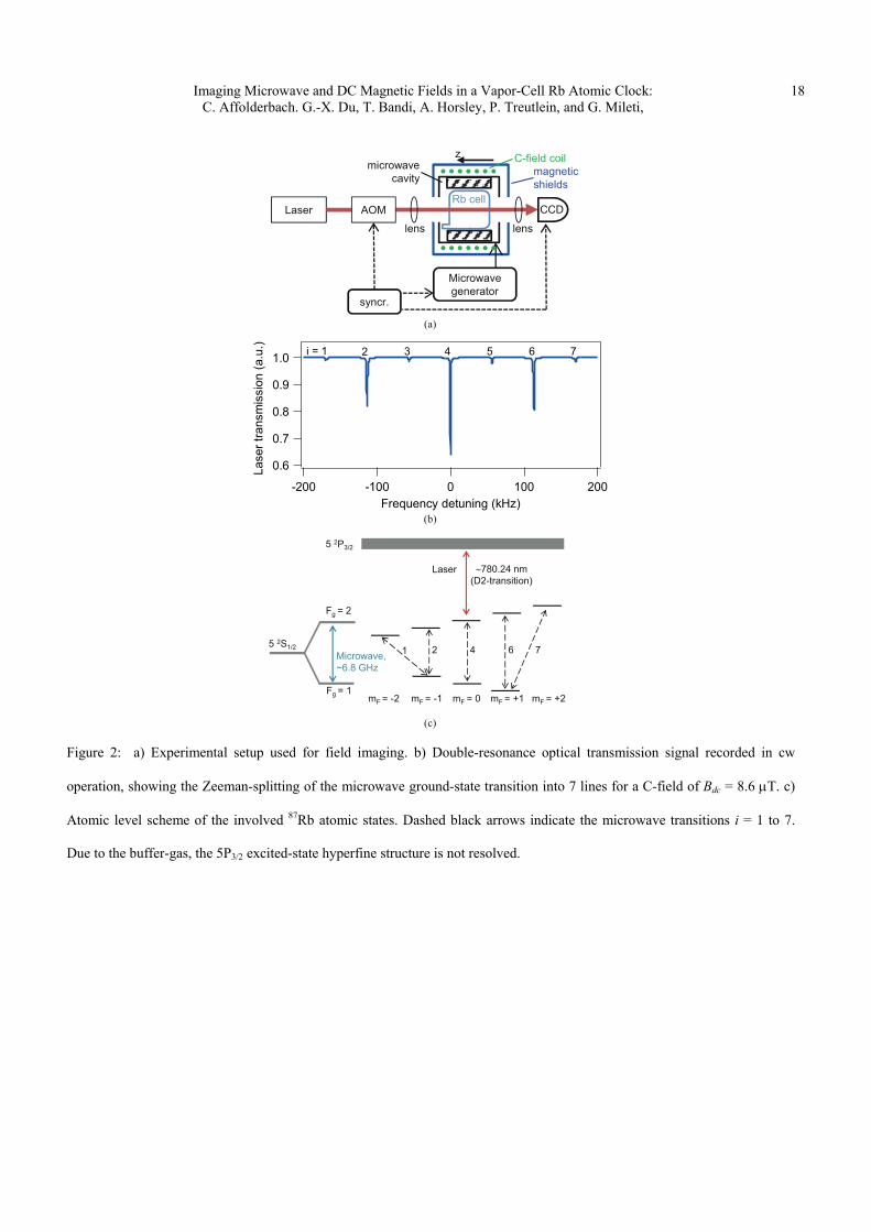
For our field imaging studies we use the modified Rb atomic clock setup shown in Fig. 2a. The microwave cavity (as described

in section II-A above) is placed inside a clock physics package also containing a thermostat, magnetic shields, and a solenoid (40

mm radius and 48 mm length) placed around the cavity for applying the DC magnetic field of Bdc ≈ 40 T, oriented parallel to

the z axis. The vapor cell is made of borosilicate glass, has a diameter and length of 25 mm each, and is equipped with a

cylindrical stem serving as Rb reservoir (see Fig. 1b). It contains isotopically enriched 87Rb, and 26 mbar buffer-gas mixture of

N2 and Ar for suppressed temperature sensitivity of the clock transition. The main cell body is held at a temperature of 55°C, and

the stem at 40°C. Under these conditions we find a mean free path of mf = 5 m for the Rb atoms in the cell.


5

Optical pumping and detection is achieved by a laser diode, whose frequency is stabilized to the Fg = 2 → Fe = 2, 3 crossover

transition of the Rb D2 line, observed in an auxiliary Rb cell without buffer gas, corresponding approximately to the center of the

collisionally broadened and shifted optical transition in the buffer-gas cell [25]. The laser intensity incident to the cavity cell was

19.7 mW/cm2, and was switched on and off using an acousto-optical modulator (AOM). The microwave radiation was produced

by a laboratory microwave synthesizer, with a frequency close to the ≈ 6.835 GHz clock transition frequency, and its pulses

controlled by switches. By setting the microwave frequency to values corresponding to the different resonances i = 1 to 7 shown

in Fig. 2b, the different Zeeman components of the Rb hyperfine ground-state transition indicated in Fig. 2c can be selected. The

typical microwave power level injected into the cavity is around +22 dBm. The laser light level transmitted through the vapor

cell is then mapped onto a CCD camera or a photodiode, using imaging optics.

C. Detection Schemes

Field imaging is performed using the method presented in [23], based on pulsed interaction schemes using Rabi measurements

and Ramsey measurements. In both schemes a first “pump” laser pulse depopulates the Fg = 2 ground-state level, followed by

one or two microwave pulses for coherent interaction, and finally a weak probe laser pulse reads out the resulting atomic

population in the Fg = 2 state. The variation in optical density OD of the atomic sample induced by the pulsed interaction

scheme is then calculated from the laser intensities transmitted through the cell as described in [23]. While in [23] imaging was

performed on a micro-fabricated vapor cell resulting in a spatial resolution in z-direction defined by the cell thickness of 2 mm,

we here apply the imaging technique to a thick cell of 25 mm length.

Rabi measurements, using one microwave pulse of variable duration dtmw between the optical pump and probe pulses, were

employed for imaging of the microwave magnetic field amplitudes in the cavity. In this case, the microwave frequency is tuned

to the center of the selected Zeeman component of the hyperfine transition. The observed variation in optical density as function

of dtmw shows Rabi oscillations and is described by

∆ exp exp sin Ω (1)


6

Here the fit parameters are an overall constant offset A in optical density, amplitude B of the relaxation of population with its

related time constant 1, and the amplitude C, time constant 2, Rabi frequency , and phase of the Rabi oscillations introduced

by the microwave field. By tuning the microwave frequency to the transitions i = 1, 4, or 7 we are sensitive to the , , or

component of the microwave magnetic field, respectively, via the corresponding transition’s Rabi frequency i

Imaging of the DC magnetic C-field was conducted using Ramsey measurements, where the microwave interaction is achieved

by two /2 microwave pulses separated by a Ramsey time dtR, during which neither light nor microwave are applied. The

detected variation in optical density as function of dtR is described by

∆ exp exp sin (2)

Here the fit parameters are A, B, C, T1, T2, , and analogue to Eq. (1), with T1 and T2 the population and coherence lifetimes,

respectively. The Ramsey oscillation frequency is equal to the microwave detuning from the atomic transition. Thus, for an

externally fixed microwave frequency injected into the cavity, the value of encodes the C- field amplitude at the position of the

sampled atoms, via the Zeeman shift of the selected transition. Using the Breit-Rabi formula [26], the C- field amplitude can then

be calculated from , and common-mode frequency shift such as buffer-gas shifts can be eliminated when combining

measurements on two different transitions.

For construction of spatially resolved images, imaging optics and a CCD camera are used for measuring the transmitted laser

intensities. Using a pattern mask at the level of the cavity as well as ray transfer matrix calculation, the imaging optics is found to

result in a 1:4 demagnification of the atoms’ image on the CCD sensor. In order to reduce noise and limit computation effort on

the fitting, the CCD images were binned into image pixels of 3x3 CCD-pixels. Each resulting image pixel corresponds to a

76 m 76 m cross section at the cell and contains the atomic signal integrated within this area. The imaged area has a

diameter of 11 mm at the cell, and each image consists of ≈15’000 image pixels. The time series OD(dtmw) or OD(dtR) are

fitted with equations (1) or (2), respectively, independently for each image pixel. For both Eq. (1) and (2), all seven fit

parameters are fitted independently. Examples of such fits to Rabi and Ramsey data of a typical single image pixel are shown in

Fig. 3, for data recorded on the i = 7 transition. Both data sets are well described by the fit functions of Eq. (1) and (2),

respectively. Finally, the fit parameters from each pixel are recombined to obtain images of the physical entities of interest.


7

Because the measurements are taking place in the time domain, the fit parameters and of main interest here are largely

insensitive to overall variations in the signal amplitude.

III. EXPERIMENTAL RESULTS

In the following we discuss the images of the DC and microwave magnetic fields across the cell, obtained with the Rabi and

Ramsey interrogation schemes. Images obtained generally refer to the x-y plane, but certain information on the field distribution

along the z-axis can also be obtained.

A. Imaging of the DC Magnetic Field

Imaging of the DC magnetic C-field was achieved using the Ramsey interrogation method (see section II-C). Figure 4 shows the

C-field amplitude Bdc and T2 lifetime images, obtained from the corresponding fit parameters of Eq. (2). Data was recorded with

the microwave frequency tuned close to the i = 2 transition and common-mode frequency shifts were removed by using similar

measurements on the i = 6 transition. The C-field amplitude is found to be very homogeneous, with a peak-to-peak variation of

only 0.13 T (or 0.3%) over the sampled cell region. Relative uncertainties returned from the fit on each individual pixel are <

0.5% for the C-field amplitude, and < 8% for the T2 time. The images of both the C-field and T2 show a circular symmetry

around the same center (indicated by black crosses in the left-hand panels of Fig.4), and do not correlate with any symmetry of

the microwave magnetic field distributions measured (see section III-B below). Images of Bdc and T2 qualitatively and

quantitatively very similar to Fig. 4 are obtained when the microwave frequency is tuned close to the transitions i = 1, 6, and 7.

Fitting uncertainties are < 1% for the C-field amplitude and on the level of 2% to 10% for T2 in all cases.

For a more quantitative analysis, we plot the C-field amplitude (Fig. 5a) and T2 (Fig. 5b) as functions of distance r from the

center of symmetry (black crosses in the left-hand panels of Fig. 4), for transition i = 2. The C-field dependence on r is well-

described by

Bdc (r) = C0 + C2·r2 + C4·r

4 (3)


8

shown as fit in Fig. 5a. As expected, the C-field profiles measured on transitions i = 1, 6, and 7 show a very similar behavior: All

4 transitions give a consistent value of Bdc (r=0) = C0 = 40.31 T, only slightly below the 40.41 T calculated from the solenoid

geometry and applied current. Because the clock transition (i = 4) shifts in second order only with the magnetic field,

determination of the C-field amplitude from this transition gives much bigger uncertainties, with data scatter on the level of

0.1 T, which completely masks the C-field structure visible in Fig. 5a.

The measured C-field amplitudes and T2 times are clearly correlated, as seen from Fig. 4. This can be attributed to

inhomogeneous dephasing due to spatial gradients in the C-field, a process well-known from nuclear magnetic resonance (NMR)

spectroscopy: at large r values, the Rb atoms diffusing through the buffer gas sample spatial regions of more pronounced

differences in C-field amplitude, thus resulting in reduced T2 times [27], [28]. Figure 5b indeed shows a general linear decrease

of T2 with r (dashed black line in Fig. 5b), with a slope ∑T2/∑r = 41.6 s/mm, which is consistent with a dependence of T2 on

the field gradient ∑Bdc/∑r for a C-field distribution governed by the quadratic term C2·r2, as is the case here. One further observes

that T2 values above (below) the linear trend are measured in regions where ∑Bdc/∑r is locally smaller (larger) than the derivative

of the general polynomial of Eq. (3), marked by dashed (solid) vertical arrows in Fig. 5a and 5b. The radial T2 profiles measured

on transitions i = 1, 6, and 7 again show the same general behavior as found for i = 2, however residual deviations from the linear

trend are slightly stronger on i = 1 and 7 (recorded using the and microwave magnetic field components) than for the i = 2

and 6 case (recorded using the microwave field component). This indicates a dependence of the inhomogeneous dephasing on

the mF quantum numbers or magnetic field component involved.

Under conditions of inhomogeneous dephasing in spin echo NMR and for linear and quadratic spatial variation of the static

magnetic field the overall transverse relaxation time T2* is given by [28], [29]

210,2

2

311

0,2

1*2 GTtGDTT R

(4)

Here T2,0 is the T2 time at vanishing field gradient, D the diffusion constant of Rb atoms in our cell, the atoms’ gyromagnetic

factor, tR the average Ramsey time, and G the local gradient of the static magnetic field of relevance here. For more complicated

field distributions, numerical approaches are generally used [30]. The solid black line in Fig. 5b gives a fit of T2*(r) according to

Eq. (4) to the measured distribution T2(r), using G(r)=dB(r)/dr calculated according to the fit of Eq. (3) shown in Fig. 5a, which


9

yields T2*(r=0) = T2,0 = 445.5(6) s and = 1.794(8) mm2·s-1· for the only two free parameters of this fit. Although

derived for the case of spin echo, this curve reproduces very well the general shape of the measured T2(r) dependence. The blue

dotted curve in Fig. 5b gives the profile T2*(r) calculated for our cell conditions, using the same T2

*(r=0) = 445.5 s and

= 1.2 mm2·s-1· (calculated from D=7.1 cm2/s for our cell conditions and tR = 0.8 ms, no free parameters). We attribute

this residual difference in to the fact that i) Eq. (4) is derived for spin echo experiments while our measurements are obtained

using the Ramsey scheme with varying tR, and ii) the actual field gradient G(r) might be underestimated by neglecting

contributions from dB(r)/dz here. The results still indicate that the observed variation T2(r) can indeed be caused by

inhomogeneous dephasing due to magnetic field gradients.

Figure 5c shows the T2 time measured on the i = 4 transition. Again, T2 shows a linear dependence on r, with a slope

∑T2/∑r = 13.3 s/mm, approximately 3 times lower than observed on i = 1, 2, 6, and 7. The mean value of T2 = 1.5(2) ms is

considerably higher than the one observed on the other transitions and is in agreement with the intrinsic clock transition

linewidth measured for this cell [31].

B. Imaging of the Microwave Field

Imaging of the microwave magnetic field inside the cavity was performed using the Rabi interrogation scheme (see section

II-C). The microwave transitions i = 1, 4, and 7 are exclusively driven by the , , and components of the microwave

magnetic field, respectively. By tuning the microwave frequency to each of these resonances in turn and extracting the

corresponding Rabi frequencies i from fits of Eq. (1) to each pixel’s data we can therefore determine the amplitude of the

magnetic microwave field components as:

131 B

B

4B

B (5)

731 B

B


10

where B, B, and B are the amplitudes of the , , and microwave field components, respectively [21]. Here, the

microwave magnetic field amplitudes are defined with respect to their Cartesian basis as [32]:

yx

yx

z

iBBB

iBBB

BB

21

21

(6)

The results obtained for the different microwave field components are shown in Fig. 6, together with the corresponding Rabi

oscillation lifetime 2. The variations of the microwave magnetic field -component are less than 20% of its peak value across

the entire image, much stronger than those detected for the C-field and not correlated with the latter. The maximum values for

the and components are on the level of 10% and 20%, respectively, of the -component’s maximum value, which confirms

a microwave magnetic field predominantly oriented parallel to the z direction [13]. Note that during clock operation, these B

and B field components can in principle induce AC Zeeman shifts of the atomic levels and thus frequency shifts of the clock (in

analogy to AC Stark shift introduced by the optical radiation). However, in clock operation the microwave frequency will be

resonant with the i = 4 -transition, and thus far off-resonant with respect to the s transitions (by approximately ≥ 30 linewidths

here), thus AC Zeeman shifts from the B component can be expected to be largely dominant. The off-center position of the field

maximum for the -component can be attributed to a shift of the microwave field distribution caused by the cell reservoir located

on the upper left rim of the cavity (see Fig. 1b) [33]. Fitting uncertainties for the microwave field amplitude are < 8 nT or < 3%

for all three field components.

Similar to the observations made in [23] and on the C-field images (section III-A) we also here see a reduction of Rabi

oscillation lifetime, i.e. inhomogeneous dephasing, but this time as a function of the microwave magnetic field amplitude: for

each field component, 2 reaches its maximum in regions where the gradient of the microwave magnetic field amplitude is small,

while 2 is lower in regions of high microwave magnetic field gradients. Fitting uncertainties for 2 are generally below 5%,

reaching up to 8% only in the region of highest 2 in the image of the component (due to the relatively short maximum dtmw

employed here).


11

In the microwave magnetic field data of Fig. 6a a small region close to the lower left edge of the imaging area exhibits some

deviations from the general structure seen. We interpret this structure as an artefact, arising from the unfavorable combination of

low magnetic field values (and thus long Rabi oscillation period) and short Rabi oscillation lifetimes 2. Such limitations can be

overcome by performing the measurements at higher microwave power levels that enable again observation of several Rabi

oscillations within the 2 time.

In order to assess the detection limit of the method, measurements were repeated on transition i = 4 for different levels of

microwave power sent into the cavity, using a photodiode as detector here. The inset of Fig. 7 shows that the square of the

measured microwave field amplitude scales linearly with the microwave power sent to the cavity, as expected. Clear Rabi

oscillations can still be observed for microwave field amplitudes as low as 0.05 T. The signal-to-noise ratio (Rabi oscillation

amplitude C over rms data scatter) found for the Rabi data of Fig. 3a, although taken on a single image pixel only, is even better

than that of Fig.7, and the difference in magnetic field amplitude detected is mainly reflected by the different time scale of the

Rabi oscillations – note the difference in x-axis scaling by a factor of 10. We therefore conclude that also in the imaging mode

microwave magnetic field amplitudes of 0.05 T or below can be detected with this method.

In principle, the images of the microwave magnetic field shown in Fig. 6 give for each image pixel an average value of the field

amplitude, integrated over the 25 mm length of our thick cell along the laser beam propagation direction (parallel to the

z-axis), which is a conceptual difference to the work in [23] on a thin cell. One can however still obtain some statistical

information on the field distribution along the z-axis here, by calculating the Fourier transform spectrum of an image pixel’s

OD data (see Fig. 3), inspired by similar techniques applied in NMR and Fourier transform spectroscopy. We illustrate this

approach for the example of the microwave field component (Fig. 6b), but it is equally applicable to the other field components

or the C-field data of Fig.4. Figure 8 shows the Fourier transform magnitude for pixels (88,98) and (39,15) of Fig. 6b, that are

from regions of high and low B amplitude, respectively, as well as for the data obtained by integrating OD over the entire

image (x and y coordinates) for each value of dtmw. The Fourier frequency axis is then scaled into microwave magnetic field

amplitude according to Eq. (5).

The resolution of the Fourier spectrum in Fig. 8 is ≈ 0.4 kHz, or 30 nT, due to the limited length of the dtmw time-domain signal

used here. Nevertheless all three Fourier spectra show narrow peaks for the B distribution, with a spread of 10% or less for the

two individual pixels. At low frequencies the spectrum diverges due to the exponential background in the time-domain signal,


12

which is of no interest here and therefore is omitted from Fig. 8. For pixel (39,15), the small peak at B< 1 T indicates the

presence of some z-region with very low field amplitude. The integrated signal shows a structure composed of the distinct

features of both extreme pixels selected, plus an intermediate feature at 4.5 T, as expected from the general field distribution in

Fig. 6b. In the integrated signal small dips are seen at 4.14, 4.3, and 4.55 T, making this signal appear to be constituted of

several distinct peaks. Given the overall smooth field distribution of Fig. 6b, these dips might well be artifacts without statistical

significance, arising from measurement noise or instabilities converted by the FFT routine employed. Note that the contribution

of the low field amplitudes like in pixel (39,15) to the integrated signal is small, due to the small image area in Fig. 6b showing

such low amplitude values. We thus conclude that also the variation of Balong the z-axis is small (< 10%), otherwise a more

pronounced broadening of the B distribution should be observable for all 3 traces in Fig.8.

C. Optical Pumping Efficiency

Figure 9 shows the image of the A parameter in Eq. (1), which is a measure of the optical pumping efficiency, for the microwave

component of Fig. 6b here. The fringes seen are rather strong, with a small-scale variation by a factor of 4, probably due to

optical interferences caused by not perfectly planar cell windows – notably at the upper left edge where the cell reservoir is

located – and by the apertures of the imaging optics. These fringes are not observed in the microwave field images of Fig. 6, and

only slightly in the 2 images and fitting uncertainties, which demonstrates the robustness of the method against variations in

light intensity. Also in the Ramsey scheme the impact of these fringes is very small, with only small distortions visible in the T2

images (see Fig. 4).


13

IV. CONCLUSION

We have employed imaging techniques based on time-domain Ramsey and Rabi spectroscopy of Rb atoms for measuring

experimentally the DC and microwave magnetic field distributions inside a compact microwave resonator holding a Rb vapor

cell. The -component of the microwave magnetic field – relevant for clock operation – is found to vary by less than 20% of its

maximum value over the entire imaging region. This level of homogeneity is expected to be sufficient for the observation of

high-contrast Ramsey fringes in pulsed clock operation [34]. The and field components – orthogonal to the -component –

show much lower peak amplitudes of 10% and 20% of the -component’s maximum value, respectively. Using Fourier

Transform analysis of the signals, information on the otherwise unresolved field distribution along the z-axis (i.e. propagation

direction of the laser beam) can also be obtained and indicates a very homogeneous distribution of the microwave -component

along the z-axis, also favorable for pulsed clock operation. Imaging of the C-field amplitude in the cell reveals <1% amplitude

variation across the cell, and along with T2 relaxation times that correlate with the gradient of the C-field amplitude, due to

inhomogeneous dephasing. Fourier analysis as demonstrated for the microwave fields can also be applied to the C-field data.

The employed imaging techniques allow assessing experimentally the DC (“C-field”) and microwave magnetic field

distributions in a vapor-cell atomic clock physics package, under real operating conditions of the fully assembled cell and

resonator package. This possibility is of particular importance for the microwave magnetic field whose distribution generally is

affected by the presence of the dielectric cell material. Given the relatively limited fabrication tolerances possible for such cells,

such in situ assessment of the microwave field distribution is of high relevance for the development of compact high-

performance vapor-cell atomic clocks or other atomic sensors. The method can also be conveniently used as a diagnostics tool

for detecting changes in C-field amplitude after extended clock operation time, due to re-magnetization or hysteresis of the

magnetic shields employed.


14

ACKNOWLEDGMENT

We thank A. K. Skrivervik and A. Ivanov (Laboratory of Electromagnetics and Acoustics (LEMA), École Polytechnique

Fédérale de Lausanne (EPFL), Lausanne, Switzerland) for many helpful discussions and support on the microwave cavity, M.

Pellaton (UniNe-LTF) for making the vapor cell, and P. Scherler (UniNe-LTF) for support on design, manufacturing and

assembly of the microwave cavity and its physics package.

REFERENCES

[1] J. Vanier and C. Audoin, “The Quantum Physics of Atomic Frequency Standards”, (Adam Hilger, Bristol, UK, 1989).

[2] J. Camparo, “The Rb atomic clock and basic research”, Physics Today, vol. 60, pp. 33 – 39, Nov. 2007.

[3] J. A. Kusters, C. J. Adams, “Performance requirements of communication base station time standards”, RF Design, vol. 5,

pp. 28 – 32, May 1999.

[4] L. A. Mallette, J. White, and P. Rochat, “Space qualified frequency sources (clocks) for current and future GNSS

applications 2010,” in Proc. Position Location and Navigation Symposium, Indian Wells, CA, USA, 2010, pp. 903-908.

[5] T. Bandi, C. Affolderbach, C. Stefanucci, F. Merli, A. K. Skrivervik, and G. Mileti, ” Compact High-Performance

Continuous-Wave Double-Resonance Rubidium Standard With 1.4 × 10−13 τ −1/2 Stability”, IEEE Trans. Ultrason.,

Ferroelectr., Freq. Control, vol. 61, no. 11, pp. 1769 – 1778, Nov. 2014.

[6] S. Micalizio, C. E. Calosso, A. Godone, and F. Levi, “Metrological characterization of the pulsed Rb clock with optical

detection”, Metrologia, vol. 49, no. 4, pp. 425 – 436, May 2012.

[7] J. Guéna, M. Abgrall, A. Clairon, and S. Bize, “Contributing to TAI with a secondary representation of the SI second”,

Metrologia, vol. 51, no.1, pp. 108 – 120, February 2014.

[8] W. Happer, “Optical Pumping”, Rev. Mod. Physics, vol. 44, no. 2, pp. 169 – 249, April 1972.

[9] B. S. Mathur, H. Tang, and W. Happer, “Light Shift in the Alkali Atoms”, Phys. Rev., vol. 171, no. 1, pp. 11 – 19, July

1968.

[10] N. F. Ramsey, “A New Molecular Beam Resonance Method”, Phys. Rev., vol. 76, no. 7, pp. 996 – 996, October 1949.

[11] G. Mileti, I. Ruedi, and H. Schweda, “Line Inhomogeneity effects and power shift in miniaturized Rubidium frequency

standards”, in Proc. 6th European Frequency and Time Forum, Noordwijk, The Netherlands, 1992, pp. 515 – 519.


15

[12] H. Chen, J. Li, Y. Liu, and L. Gao, “A study on the frequency–temperature coefficient of a microwave cavity in a passive

hydrogen maser”, Metrologia, vol. 49, no. 6, pp. 816 – 820, Nov. 2012.

[13] C. Stefanucci, T. Bandi, F. Merli, M. Pellaton, C. Affolderbach, G. Mileti, and A. K. Skrivervik, “Compact microwave

cavity for high performance rubidium frequency standards”, Rev. Sci. Instrum., vol. 83, no. 10, pp. 104706, Oct. 2012.

[14] T. Bandi, C. Affolderbach, C. E. Calosso, and G. Mileti, High-Performance Laser-Pumped Rubidium Frequency Standard

for Satellite Navigation, Electronics Letters, vol. 47, no. 12, pp. 698 – 699, June 2011.

[15] A. Godone, S. Micalizio, F. Levi, and C. Calosso, “Microwave cavities for vapor cell frequency standards”, Rev. Sci.

Instrum., vol. 82, no. 7, pp. 074703, July 2011.

[16] B. Xia, D. Zhong, S. An, and G. Mei, “Characteristics of a novel kind of miniaturized cavity-cell assembly for rubidium

frequency standards”, IEEE Trans. Instrum. Meas., vol. 55, no. 3, pp. 1000–1005, Jun. 2006.

[17] M. Violetti, M. Pellaton, F. Merli, J.–F. Zürcher, C. Affolderbach, G. Mileti, A. K. Skrivervik, “The Micro Loop-Gap

Resonator: A Novel Miniaturized Microwave Cavity for Double-Resonance Rubidium Atomic Clocks”, IEEE Journal of

Sensors, vol. 14, no. 9, pp. 3193 – 3200, Sept. 2014.

[18] R. Li and K. Gibble, “Evaluating and minimizing distributed cavity phase errors in atomic clocks”, Metrologia, vol. 47, no.

5, pp. 534 – 551, August 2010.

[19] R. P. Frueholz, C. H. Volk, and J. C. Camparo, “Use of wall coated cells in atomic frequency standards”, J. Appl. Phys., vol.

54, pp. 5613 – 5617, Oct. 1983.

[20] A. Risley, S. Jarvis, and J. Vanier, “The Dependence of Frequency Upon Microwave Power of Wall-coated and Buffer-gas-

filled Gas Cell Rb87 Frequency Standards”, J. Appl. Phys., vol. 51, pp. 4571 – 4576, Sept. 1980.

[21] P. Böhi, M. F. Riedel, T. W. Hänsch, and P. Treutlein, “Imaging of microwave fields using ultracold atoms”, Appl. Phys.

Lett., vol. 97, no. 5, pp. 051101, April 2010.

[22] P. A. Böhi and P. Treutlein,“ Simple microwave field imaging technique using hot atomic vapor cells”, Appl. Phys. Lett.,

vol. 101, no. 18, pp. 181107, Oct. 2012.

[23] A. Horsley, G.-X. Du, M. Pellaton, C. Affolderbach, G. Mileti, and P. Treutlein, “Imaging of Relaxation Times and

Microwave Field Strength in a Microfabricated Vapor Cell”, Phys. Rev. A, vol. 88, 063407, Oct. 2013.

[24] W. Froncisz and J. S. Hyde, “The Loop-Gap Resonator: A New Microwave Lumped Circuit ESR Sample Structure”, J.

Magn. Reson., vol. 47, pp. 515 – 521, February 1982.

[25] M. D. Rotondaro and G. P. Perram, ”Collisional Broadening and Shift of the Rubidium D1 and D2 Lines by Rare Gases, H2,

D22, N2, and CF4”, J. Quant. Spectrosc. Radiat. Transfer, vol. 57, no. 4, pp. 497 – 507, 1997.


16

[26] G. Breit and I. I. Rabi, “Measurement of Nuclear Spin”, Phys. Rev., vol. 38, no. 11, pp. 2082 – 2083, Dec. 1931.

[27] H. Y. Carr and E. M. Purcell, “Effects of Diffusion on Free Precession in Nuclear Magnetic Resonance Experiments”, Phys.

Rev., vol. 94, no. 3, pp. 630 – 638, May 1954.

[28] H. C. Torrey, “Bloch Equations with Diffusion Terms”, Phys. Rev., vol. 104, no. 3, pp. 563 – 565, November 1956.

[29] P. Le Doussal and P. N. Sen, “Decay of nuclear magnetization by diffusion in a parabolic magnetic field: An exactly

solvable model”, Phys. Rev. B, vol. 46, no. 6, pp. 3465 – 3486, August 1992).

[30] C. H. Ziener, S. Glutsch, P. M. Jakob, and W. R. Bauer, “Spin dephasing in the dipole field around capillaries and cells:

Numerical solution”, Phys. Rev. E, vol. 80, no. 4, pp. 046701, October 2009.

[31] T. Bandi, “Double-Resonance Studies on Compact High-performance Rubidium Cell Frequency Standards”, PhD

dissertation, University of Neuchâtel, Neuchâtel, Switzerland, 2013.

[32] For details on the definitions of the fields and Rabi frequencies used in our formalism, see the supplementary material to

[21], available online at http://dx.doi.org/10.1063/1.3470591.

[33] A. Ivanov, T. Bandi, G.-X. Du, A. Horsley, C. Affolderbach, P. Treutlein, G. Mileti, and A. K. Skrivervik, “Experimental

and numerical study of the microwave field distribution in a compact magnetron-type microwave cavity”, in: proceedings of

the 28th European Frequency and Time Forum (EFTF), Neuchatel, Switzerland, June 22 - 26, 2014, pp. 208 – 211.

[34] S. Kang, C. Affolderbach, F. Gruet, M. Gharavipour, C. E. Calosso, G. Mileti, “Pulsed Optical Pumping in a Rb Vapour

Cell Using a Compact Magnetron-Type Microwave cavity”, in: proceedings of the 28th European Frequency and Time

Forum (EFTF), Neuchatel, Switzerland, June 22 - 26, 2014, pp. 545-547.


17

Figure 1: a) Cross-section drawing of the microwave cavity with its electrode structure. The coordinate system used

throughout the paper is shown; the z-axis coincides with the cavity’s axis of cylindrical symmetry. b) Assembled microwave

cavity with the Rb vapor cell. For better visibility, the coordinate system is offset from its true origin here.

(a) (b)

xz

y

xz

y


18

Figure 2: a) Experimental setup used for field imaging. b) Double-resonance optical transmission signal recorded in cw

operation, showing the Zeeman-splitting of the microwave ground-state transition into 7 lines for a C-field of Bdc = 8.6 T. c)

Atomic level scheme of the involved 87Rb atomic states. Dashed black arrows indicate the microwave transitions i = 1 to 7.

Due to the buffer-gas, the 5P3/2 excited-state hyperfine structure is not resolved.

Fg = 2

Fg = 1

5 2S1/2

5 2P3/2

mF = +2mF = -2 mF = -1

∼780.24 nm(D2-transition)

Laser

4Microwave, ~6.8 GHz

2 61 7

Laser CCD

Microwave generator

AOM

syncr.

Rb cell

lenslens

microwave cavity

z C-field coil

(b)

(c)

(a)

magneticshields

mF = 0 mF = +1


19

Figure 3: Typical examples of time-domain oscillations in the CCD signal, recorded on the i = 7 transition here. a) Rabi data for

image pixel (80,80) from Fig. 6c, corresponding to a microwave magnetic field amplitude B = 0.5 T. b) Ramsey data for an

image pixel at the center of symmetry, from data similar to that of Fig. 4. Insets show the pulse sequences employed. In both

Figs. 3a and 3b the signals are normalized such that OD= 0 corresponds to the cell’s optical density under conditions of optical

pumping but without any microwave interaction applied.

(a)

(b)

on

offlaser

microwave dtmw

pump probe

on

off

on

offlaser

microwave dtR

pump probe

on

off


20

Figure 4: Imaging results measured on transition i = 2 (mF=1 = 1 → mF=2 = ). Upper left panel: DC magnetic field

amplitude Bdc. Lower left panel: T2 times. Right-hand panels: corresponding uncertainties returned from the fitting routine.

Black crosses in the left-hand panels give the centers of circular symmetry found for both images. See Fig. 1 for definition of

the coordinate system used.

X (mm)

Y (m

m)

−5 0 5−5

0

5

40.3

40.35

40.4

X (mm)

−5 0 5−5

0

5

0.1

0.2

0.3

0.4

X (mm)

−5 0 5−5

0

5

300

400

500

X (mm)

−5 0 5

0

5

2

4

6

8

Bdc (μT) ΔBdc (%)

T2 (μs) ΔT2 (%)Y

(mm

)Y

(mm

)

Y (m

m)

−5

+

+


21

Figure 5: a) radial profile of the C- field amplitude measured on transition i = 2 (dots) and 4th-order polynomial fit to the data

(solid line), b) radial profile of the corresponding T2 time, measured on the i = 2 transition. Solid arrows mark regions of

locally higher c-field gradient and relatively lower T2 times, and dashed arrows mark regions of opposite characteristics. c)

radial profile of the T2 time measured on the i = 4 transition.

��

��

��

��

��

��

��

��

��

��

��

��

��

��

��

��

��

��

��

��

��

��

��

��

!�

"�

�� "��"#��


22

Figure 6: Imaging results for the amplitude B, B, B of the three microwave magnetic field components and corresponding

Rabi oscillation lifetimes 2. a) component, measured on transition i = 1 (mF=1 = 1 → mF=2 = ); b) component, measured

on transition i = 4 (mF=1 = 0 → mF=2 = 0); c) component, measured on transition i = 7 (mF=1 = +1 → mF=2 = +2). Note the

difference in color scale between the sub-panels. Uncertainties for the microwave magnetic field amplitude and Rabi oscillation

lifetimes are shown for the component only (sub-panel b), but are similar for the components. The white and black circle in

sub-panel b indicate the pixels (88,98) and (39,15), respectively, used for the Fourier analysis of Fig. 8. The white circle in sub-

panel c indicates pixel (80,80) used in Fig. 3a.

X (mm)

Y (m

m)

−5 0 5−5

0

5

4

4.2

4.4

4.6

4.8

X (mm)

Y (m

m)

−5 0 5−5

0

5

0

0.05

0.1

X (mm)

Y (m

m)

−5 0 5−5

0

5

200

400

600

X (mm)Y

(mm

)

−5 0 5−5

0

5

0

2

4

6

8

Bπ (μT) ΔBπ (%)

τ2 (μs) Δτ2 (%)

X (mm)

Y (m

m)

−5 0 5−5

0

5

0

0.1

0.2

0.3

0.4

B+ (μT)

X (mm)

Y (m

m)

−5 0 5−5

0

5

0

200

400

600

τ2 (μs)

X (mm)

Y (m

m)

−5 0 5−5

0

5

0.2

0.4

0.6

0.8

X (mm)

Y (m

m)

−5 0 5−5

0

5

0

50

100

150

200

τ2 (μs)

(a) σ− component

B- (μT)

(c) σ+ component(b) π component

Figure 7: Rabi oscillations can still be clearly observed for a microwave field amplitude as low as B = 0.047 T (microwave

power of Pmw=1.5 W sent to the cavity). The square B2 of the microwave field amplitude scales linearly with the microwave

power Pmw sent to the cavity, see inset.

��

��

��

��

��

��

��

��

��

��

��

!�"�� #��$%��&��

��!�"�� #� � �� "�#��' ��(�

��


23

Figure 8: Relative contribution of the different field amplitudes for the microwave field component (see Fig. 6b), obtained by

Fourier transform analysis of the OD(dtmw) signal. Solid black line: signal integrated over the entire image; dashed red line:

pixel (88,98) with high B; dotted blue line: pixel (39,15) with low B. The position of the selected pixels is shown in Fig. 6b.

For better visibility, the FFT magnitudes of pixel (39,15) and for the integrated signal were multiplied by factors of 2 and 15,

respectively, to compensate differences in FFT magnitudes caused by the different T2 times of the time-domain signals.

�

�

�

�

�

��

�� !� � �"� #" ��

�� $ ��"# %�" ��&'��# %�" ��'&��

Figure 9: Image of fit parameter A of equation (1) for Rabi images of the microwave magnetic field component shown in Fig.

6b.

X (mm)

Y (m

m)

−5 0 5−5

0

5

0

1

2

3

4

A

imaging microwave and dc magnetic fields in a vapor … microwave and dc magnetic fields in a...

Documents