image restoration based on edgemap and wiener … from the noisy image by using a new edge ... other...

Abstract—This paper presents a method for removing noise while preserving the image fine details and edges in blind condition, based

on the Wiener filter and a constructed edgemap. The noisy image is denoised with different weights of Wiener filtering to generate two restored images; one with highly reduced noise, and the other with preserved fine details and edges. The edgemap image is constructed directly from the noisy image by using a new edge detection method. The Wiener filtered images and the edgemap are utilized to generate the final restored image. Simulations with natural images contamina- ted by noise demonstrate that the proposed method works effectively

over a different range of noise levels. A performance comparison with other Wiener filter-based denoising methods and the state-of-the-art denosing methods is also made.

Keywords— Edgemap, Image denoising, Power spectrum

estimation, Wiener filter.

I. INTRODUCTION

LTHOUGH image denoising has been researched quite

extensively, developing a denoising method that could

remove noise effectively without eliminating the image fine

details and edges is still a challenging task. Until recent years,

many denoising methods have been proposed [1]-[5]. Some

recent non-linear methods suggest employing different denois-

ing approaches for the smooth and non-smooth regions. This

type of technique is proposed in the adaptive Total Variation

(ATV) [3] and the non-local means (NLM) [4] methods. Con-

versely, linear methods such as the Wiener filter [6] balance the

tradeoff between inverse filtering and noise smoothing. The

Wiener filter eliminates the additive noise while inverting

blurring.

The Wiener filter is the best known technique for the linear

image denoising [7]. It has been implemented for image denois-

ing in several transform domains, for example the spatial

domain [8],[9], and the frequency domain [10],[11]. Recently,

the wavelet-based denoising methods have dominated the latest

research trend in image processing. The Wiener filter

This study was supported and sponsored by Saitama University, Malaysia

Ministry of Higher Education (MOHE) and Tun Hussein Onn Malaysia

University (UTHM).

S. Suhaila is with the Graduate School of Science and Engineering, Saitama

University, Saitama, Japan, 338-8570 (phone: 81-48-858-3496; fax: 81-48-858

-3716; e-mail: [email protected]).

T. Shimamura is with the Graduate School of Science and Engineering,

Saitama University, Saitama, Japan, 338-8570 (e-mail: [email protected]

-u.ac.jp).

implemented in the wavelet domain by using the first generation wavelet has been introduced in many papers, for

example in [12],[13]. The second generation wavelet: lifting-

based wavelet has been introduced by Sweldens [14] to help

reducing computation, which also achieves lossy to lossless

performance with a finite precision [15]. The lifting-based

wavelet domain Wiener filter (LBWDWF) [16] shows substan-

tial improvement in the restoration performance, and provides

much faster computation in comparison to the classical wavelet

domain Wiener filter [18]. In practical cases, the information of

the original image and the noise level is unknown (blind

condition). Thus, to utilize the Wiener filter, noise estimation

plays an important role to accomplish accurate denoising. The

Wiener filter applied in the spatial domain, the adaptive Wiener

filter (AWF), as suggested by Lee [8], first estimates the local

variances from the neighborhood around each pixel. The

average of these estimates is subsequently used to estimate the

noise variance. Methods to estimate the noise variance for the

spatial domain Wiener filter are also proposed in [17],[18].

Alternatively, several power spectrum estimation methods have

been proposed for estimating noise in the frequency domain

[19]-[22]. However, there are a few applied for direct imple-

mentation in the frequency domain Wiener filter [10], [11].

The ATV utilizes the idea of the Total Variation (TV) [23].

The TV searches for the minimal energy functional to reduce

the total variation of the image via a global power constraint.

On the other hand, the ATV reduces the total variation of the

image adaptively. It employs strong denoising in the smooth

regions and weak denoising in the non-smooth regions. The

NLM measures the similarity of the grey level between two

pixels. It also compares the geometrical configuration adapted

to the local and non-local geometry of the whole image. The

methods such as the LBWDWF, ATV and NLM are reported to

have superior performance in noise removal and preservation

of strong edges. They, however, share a common drawback:

that is, the fine details and edges of the original image are not

well preserved in the restored image, especially in higher noise

environments.

To overcome this problem, a frequency domain Wiener

filter-based denoising has been proposed in [20]. We refer this

method to as the frequency domain Wiener filter (FDWF). The

FDWF introduces a noise and image power spectra estimation

method for the implementation of the Wiener filter in blind con-

dition. The FDWF provides the preservation of the fine details

and edges, but a certain level of noise remains in the restored

Image Restoration Based on Edgemap and

Wiener Filter for Preserving Fine Details and

Edges

S. Suhaila, and T. Shimamura

A

INTERNATIONAL JOURNAL OF CIRCUITS, SYSTEMS AND SIGNAL PROCESSING

Issue 6, Volume 5, 2011 618

image.

In this paper, we propose a denoising technique to preserve

the image fine details and edges while effectively reducing the

noise level. The proposed method is based on the FDWF. The

image restored by using the FDWF with a low threshold value

is utilized in the non-smooth regions in the final restored image.

Conversely, the image restored by using the FDWF with a high

threshold value is employed in the smooth regions in the final

restored image. A new edge detection method is derived and

incorporated in the proposed method to distinguish between the

smooth and non-smooth regions effectively in the presence of

noise. The edge detection is performed in four directions and

the results are combined to construct an edgemap. The final

restored image is constructed by assigning the smooth and

non-smooth regions based on the edgemap. Simulation results

verify a significant reduction of the noise level in the smooth

regions relative to that of the FDWF.

The paper is organized as follows. We begin with the intro-

duction of the FDWF in Section II, and then describe the

proposed denoising method in Section III. In Section IV, we

discuss the simulation results and the performance comparison

of our method. In Section V, we draw concluding remarks.

II. FDWF

Our procedure for image denoising utilizes the FDWF

proposed in [24]. We assume that the image is corrupted by

independent additive zero-mean Gaussian white noise. A noisy

image, h(u,v), corrupted by the noise, n(u,v), can be expressed

as

h(u,v) = p(u,v) + n(u,v) (1)

where p(u,v) represents the original image. The FDWF

employs a threshold process to estimate the image and noise

power spectra. The assumption is that in general, the noise

power spectrum usually occupies high frequencies, and conver-

sely the image power spectrum is commonly concentrated at

low frequencies. First, we transform the noisy image h(u,v) to the frequency

domain, ɦ(s,t), by using the fast Fourier transform (FFT). The

power spectrum of ɦ is obtained by

ɦ (2)

and the logarithmic power spectrum of is given

by

(3)

We perform the estimation for the power spectra of the

image and noise block-by-block. and are assumed

as blocks. They are divided into non-overlapping sub-

blocks. and correspond to the (i,j)th sub-

block of and respectively.

Fig.1 Average of four corners (highest frequencies)

Next, we compute the average of the logarithmic power

spectrum in each sub-block, which is denoted as

, respectively. We find from all the image’s sub-blocks

the that represent the minimum and median values of

the entire as and , respectively. The mi-

nimum value and the median value are substi- tuted in the following global threshold value as

where denotes a division ratio of , and corresponds to the threshold value used for the power spectrum estimation.

The frequencies that are higher than correspond to the low

frequency regions, while those smaller than correspond to the

high frequency regions. The is essential to adjust the specific

fraction of the median value . When is set to be low,

the threshold value will be low, thus more frequencies will be

included into low frequency regions. Conversely, if is set to

be high, the threshold value will be high, thus more

frequencies will be included into high frequency regions.

Therefore, plays an important role in the threshold value deci-

sion.

The utilization of in (4) is attributed to the fact that the median represents where most of the power spectrum

concentrated. If the division of the high and low frequencies

considers the main power concentration via median, the thres-

hold value will be robust to the variation of the power spectrum

characteristics in different images.

The noise power spectrum is estimated from both high and

low frequency regions, since we consider that the noise

occupies both regions. In high frequency region, the image

power spectrum, and the noise power spec-

trum, in the corresponding sub-block are approxima-

ted by

if

then

In low frequency region, and are estimated

as

if

then

average



where the average [] represents the averaging of the sub- blocks in the four corners being at the highest frequencies.

These four sub-blocks are assumed to be occupied only by

noise. Fig. 1 illustrates the described four corners in the case of

k=8.

Finally, we perform the Wiener filtering operation. The

Wiener filter, is obtained by

The power spectrum estimation method in this paper

utilizes the image-wide Fourier transform instead of the

localized Fourier transform. If this estimation employs the

localized Fourier transform (by dividing the image into sub-

blocks, and calculating the power spectrum of each sub-block

(see Fig. 2(b)), the four corners in the sub-blocks do not

always represent the highest frequencies of the whole image.

For example, the sub-blocks containing the hat’s feathers in

Fig. 2(a) have a wide spread of energy at all frequencies.

Therefore, if the four corners of these sub-blocks are considered as noise, this will lead to incorrect noise estimation.

Conversely, the image-wide Fourier transform generates the

power spectrum with the frequencies in the outmost image

regions mostly occupied by noise. Therefore, the power

spectrum of the outmost image regions are considered to be

beneficial for the noise estimation.

In [24], the parameters k and are set to be 32 and 5,

respectively. This is due to that when =5, it provides a robust

and optimal restoration result for the FDWF in term of image

fine details and edges preservation for different image charac-

teristics and noise levels. When is fixed to 5, the threshold

value will be low. This setting will include higher frequencies

in the estimated image power spectrum. It will contribute to the

preservation of the image fine details and edges that usually

occupy higher frequencies. Fig. 3 shows the close-up view of

the restored Cameraman image and its logarithmic power spec-

trum (corrupted by the white noise with the variance, , of

225) by using the FDWF with =5. From Fig. 3 we can observe

that the FWDF has preserved the fine details and edges success-

fully, but has not effectively eliminated the noise in the restored

image.

III. PROPOSED ALGORITHM

The method proposed in this paper reduces the noise in the

image restored by using the FDWF with different parameters in

the smooth and non-smooth regions. From our investigation,

high threshold value setting in the FDWF reduces noise level.

Conversely, low threshold value setting preserves the fine de-

tails and edges. We set out to improve the FDWF restoration

performance by utilizing the advantage of both threshold

settings. Fig. 4 shows a block diagram of our method. First, the

noisy image is denoised with different weights of Wiener filter-

ing to generate two restored images; one with highly reduced noise, and the other with preserved fine details and edges. Then,

an edgemap image is generated directly from the noisy image.

The two Wiener filtered images are utilized for the non-smooth

and smooth regions based on the edgemap to generate the final

restored image.

(a) (b)

Fig. 2 (a) Lenna is divided into sub-blocks (k=8); (b) localized Fourier transform for each sub-block of (a)

(a) (b)

Fig. 3 Restored Cameraman and its logarithmic

power spectrum ( =225) by using FDWF ( =5)

Fig. 4 Block diagram of proposed method



A. Image Restoration for Non-Smooth Regions

The image restored by the FDWF with =5 is inverse

transformed to the spatial domain and represented as

hereafter. The is utilized for the non-smooth regions in

the final restored image, since it preserves the fine details and

edges effectively.

B. Image Restoration for Smooth Regions

An image with highly reduced noise, which is restored by

using the FDWF with high setting, is employed for the

smooth regions in the final restored image. If is set to be high,

the threshold value will be high. This will allow the FDWF to

threshold only the concentrated part of the low frequencies,

which is assumed to be occupied only by the image power spectrum.

The most suitable setting that provides a restored image

with considerably low noise level is selected by visual effects

evaluation. From the preliminary investigation, we found that

the FDWF with =10 provides the most suitable restored image.

The restored image of Cameraman is shown in Fig. 5. From Fig.

5 we can observe that the noise level has been effectively redu-

ced since noise is mostly cut out. On the other hand, the image

is blurred since the edges in higher frequencies are cut out as

well. Obvious ringing effects can be observed in the restored

image, which is caused by sharp discontinuities at the threshold

cutoff in the frequency domain. When the image is inverted into

the spatial domain, it generates decreasing oscillations as it

progresses outward from the center. The higher the threshold

value, the stronger the oscillations will be.

To overcome the ringing effects, we multiply the output

power spectrum filtered by the Wiener filter with a Gaussian

lowpass filter, to soften the threshold cutoff. The resto-

red image is inverse transformed to the spatial domain and

denoted as In Fig. 6, the ringing effects as seen in Fig.

5 are successfully suppressed. From our investigation, the best

parameter settings for the Gaussian lowpass filter are fixed to

the size of with the standard deviation of 10.

C. Edgemap Construction

Next, the decomposition of the smooth and non-smooth

regions is performed pixel-by-pixel based on an edgemap. This

process has two advantages. First, the process is implemented without pre-processing, where the edgemap is constructed by

executing edge detection directly from the noisy image in the

spatial domain. Secondly, it requires minimum parameter set-

ting, which is only the sub-block size for the image division.

The process of the edgemap construction is as follows.

First, the noisy image is divided into non-overlapping

sub-blocks (k=32), each of which consists of pixels. Next,

the pixel value range, of each sub-block (sub-blocks

number = ) is calculated as

-

where and are the maximum and minimum values of the pixels in the corresponding sub-block, respec-

tively. Then, the that represents the minimum value

of the entire denoted as R, is determined by

(a) (b)

Fig. 5 Restored Cameraman and its logarithmic

power spectrum ( =225) by using FDWF ( =10)

(a) (b)

Fig. 6 Result for restored Cameraman ( =225) by using

FDWF ( =10) multiplied with Gaussian lowpass filter

(a) horizontal, (b) vertical,

c ˚ d − ˚

(e) edgemap (f) noisy Lenna

Fig.7 Edgemap constructions in four directions and combined

edgemap for noisy Lenna ( =225)



min

The sub-block with minimum value is assumed to be

homogeneous and represents the smooth region in the noisy

image. The edge detection is performed along a direction. Due to

this, it will provide a more precise distinction between edges

and noise in noisy environments because isolated pixels can be

detected easier. The edge detection is performed in four direc-

tions. Four binary images are constructed from the edge detec-

tion in the horizontal, vertical, ˚ and − ˚ directions, which

are defined as and respec-

tively. The binary images specifically are obtained as

or

or

or

or

In order to determine whether a pixel in the noisy image

belongs to a line along the edges, smooth region or additive

noise, we consider the difference of corresponding pixel,

h(u,v) and its two neighbouring pixels in a direction. The

distances are compared with R. For example, in horizontal

direction as in (10), the difference between - and

and the difference between and are

calculated. If any of the two differences is larger than R, the

pixel h(u,v) is considered as a part of a line along the edges. If

both two differences are lower than R, the corresponding pixel

h(u,v) is assumed to belong to the smooth region or to be a pixel isolated from other non-smooth region’s pixel (consider-

ed as noise).

As can be observed from Fig. 7 ((a)-(d)), the edges have

been successfully detected from different directions, regardless

of the high noise level (see Fig. 7(f)). However, the edge detec-

tion from only a single direction is not sufficient to represent all

the edges for the entire image. Thus, we suggest to combine the

edge detections of all four directions for obtaining a better

result. The combined edgemap, is constructed by

=

or or or

(a) noisy Woman ( =25) (b) noisy Woman ( =100)

(c) edgemap ( =25) (d) edgemap ( =100)

(e) restored ( =25) (f) restored ( =100)

Fig. 8 Denoising for Woman image by using proposed method

Fig.7(e) shows the edge detection of the Note

that the provides relatively better edge detection along the lines in comparison with that of the single direction

edge detection.

A. Edgemap-Based Image Restoration

The final restored image, , is constructed based on the

edgemap as

. (15)

If the is equal to 0, then the (u,v)th pixel of the

final restored image is assumed as the smooth region,

and the (u,v)th pixel value of is assigned to .

Otherwise, the (u,v)th pixel value of is assigned to

. Fig. 8 shows the edgemap constructed directly from the

noisy Woman image with =25 and 100, respectively. Note

that by employing the edge detection approach in this paper, the edge detection has successfully distinguished most of the edges

from noise in different noise levels. The edges are remained

preserved while noise levels in smooth regions are better

suppressed.

IV. RESULTS AND DISCUSSION

We have tested our method on nine grayscale test images

from the SIDBA database. All images are contami-



nated with additive Gaussian white noise ( =25 and 100, and 225). The Airplane, Girl, Lenna, Woman and Boat images re-

present smooth natural images. The Barbara, Building,

Lighthouse and Text images represent natural images that are

highly rich in both fine details and edges. We investigate the

performance of our method by using the mean measure of

structural similarity (MSSIM) [25] since it is an image quality

metric that well matches the human visual perception [25]. We

also analyze the visual effects of the images. Each denoising

method for comparison processes the test images with the same

parameters setting (no tuning of parameters was performed for different noise level or image type).

We have compared our method to two Wiener filters in

different domains: the LBWDWF [16] and FDWF [24] in blind

condition. In this paper, the LBWDWF with 4 vanishing

moments (db4) lifting-based wavelet transform utilizes 3 de-

composition levels and filtering window. The FDWF

employs the setting as in Section II. The objective evaluation

results are tabulated in Tables I-III. Our method clearly

outperforms the other two methods over the entire range of

noise levels. Fig. 9(b)-(c) to Fig. 14(b)-(c) provide a visual

comparison of tested images denoised using these two algorithms. Our method is capable to reduce more noise compared

to the FDWF and provides better preservation of the original

image features than that of the LBWDWF.

Finally, we have also compared our method to two

state-of-the-art methods: the ATV [3] and NLM [4]. They are

reported to have significant performance in preserving details

while eliminating the noise. Both denoising methods are per-

formed in ideal condition, where the noise variances are known.

Conversely, our method estimates the noise employing the

approach as in Section III. We perform the ATV based on the

MATLAB code (default setting) as in [3]. In [4], the NLM

suggested using the search window size of and simi-

larity window of for images with the size of .

However, the parameters setting as in [4] results in over-

smoothed restored images for small resolution test image

( ). Thus, we set the search window and similarity

window for the NLM to and , respectively for obtain-

ing better denoising results. From Tables I-III, note that our

method is better than the ATV in most of the cases. Our method

is also better than the NLM in many images that are highly rich in both fine details and edges. Fig. 9(e)-(f) to Fig. 14(e)-(f)

provide a visual comparison of tested images denoised using

these two algorithms. In higher noise level, as can be seen in

Fig. 11(e)-(f) and Fig. 14(e)-(f), the ATV and NLM result in

strong noise removal. However, they eliminate the fine details

and edges at the same time. Our method reduces a considerable

amount of noise and furthermore preserves fine details and

edges better than the NLM and ATV. The investigation vali-

dates that our method with the proposed noise estimation

technique provides a comparable performance with the state-

of-the-arts methods performed in ideal condition. Table IV shows the execution time for each denoising

method implemented in MATLAB computed on a 1.4 GHz

Intel Core 2 Duo CPU. The execution time of our method is

slightly higher than that of the LBWDWF, but considerably

lower when compared to that of the ATV and NLM.

(a) Original (b) FDWF

(c) LBWDWF (d) Proposed

(e) ATV (f) NLM

Fig. 9 Restoration comparison of Lighthouse with

low noise level ( =25)





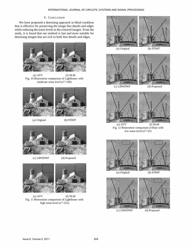
V. CONCLUSION

We have proposed a denoising approach in blind condition that is effective for preserving the image fine details and edges

while reducing the noise levels in the restored images. From the

study, it is found that our method is fast and more suitable for

denoising images that are rich in both fine details and edges.

(e) ATV (f) NLM


moderate noise level ( =100)



(e) ATV (f) NLM


high noise level ( =225)



(e) ATV (f) NLM

Fig. 12 Restoration comparison of Boat with

low noise level ( =25)





(e) ATV (f) NLM

Fig. 13. Restoration comparison of Boat with

moderate noise level ( =100)



(e) ATV (f) NLM

Fig. 14. Restoration comparison of Boat with

high noise level ( =225)

REFERENCES

[1] C. H. Hsieh, P. C. Huang and S. Y. Hung, “Noisy image restoration

based on boundary resetting BDND and median filtering with

smallest window ” WSEAS Trans. Signal Processing, vol.5, no.5, pp.

178–187, May 2009.

[2] V. Gui and C Caleanu “On the effectiveness of multiscale mode

filters in edge preserving ” in Proc. WSEAS Int. Conf. Systems,

Rodos Island, 2009, pp. 190–195.

[3] G. Gilboa, N. Sochen, and Y. Zeevi “Texture preserving variational

denoising using an adaptive fidelity term ” in Proc. IEEE Workshop

Variational and Level Set Methods in Computer Vision, Nice, 2003,

pp.137–144. Available:http://visl.technion.ac.l/~gilboa/PDE-filt/

demo.adap. tv.m.

[4] A. Buades, B. Coll and J M Morel “A non-local algorithm for image

denoising ” in Proc. IEEE Int. Conf. Computer Vision and Pattern

Table I Performance comparison in MSSIM ( =25)

Test images LBW

DWF

(blind)

FD

WF

(blind)

Propo

-sed

(blind)

ATV

(ideal)

NLM

(ideal)

Barbara 0.67 0.95 0.96 0.94 0.97

Building 0.62 0.96 0.96 0.96 0.96

Lighthouse 0.68 0.91 0.94 0.90 0.93

Text 0.68 0.95 0.96 0.95 0.93

Airplane 0.81 0.89 0.92 0.95 0.94

Girl 0.82 0.91 0.92 0.91 0.93

Lenna 0.83 0.91 0.94 0.96 0.96

Woman 0.81 0.91 0.94 0.95 0.95

Boat 0.79 0.93 0.94 0.93 0.96

Table II Performance comparison in MSSIM ( =100)

Test images

LBW

DWF

(blind)

FD

WF

(blind)

Propo

-sed

(blind)

ATV

(ideal)

NLM

(ideal)

Barbara 0.66 0.88 0.90 0.90 0.93

Building 0.62 0.89 0.91 0.90 0.91

Lighthouse 0.67 0.80 0.86 0.90 0.89

Text 0.68 0.88 0.89 0.90 0.88

Airplane 0.80 0.77 0.85 0.92 0.91

Girl 0.81 0.83 0.87 0.81 0.89

Lenna 0.82 0.82 0.88 0.92 0.92

Woman 0.80 0.82 0.87 0.90 0.91

Boat 0.78 0.84 0.88 0.86 0.92

Table III Performance comparison in MSSIM ( =225)

Test images

LBW

DWF

(blind)

FD

WF

(blind)

Propo

-sed

(blind)

ATV

(ideal)

NLM

(ideal)

Barbara 0.66 0.82 0.85 0.41 0.84

Building 0.61 0.84 0.84 0.56 0.76

Lighthouse 0.66 0.72 0.79 0.75 0.79

Text 0.67 0.82 0.84 0.72 0.80

Airplane 0.78 0.70 0.78 0.58 0.86

Girl 0.80 0.77 0.81 0.55 0.82

Lenna 0.81 0.75 0.84 0.5 0.86

Woman 0.79 0.75 0.83 0.47 0.84

Boat 0.76 0.77 0.82 0.52 0.84

Table IV Average time execution (s)

Noise,

LBW

DWF (blind)

FD

WF (blind)

Propo

-sed (blind)

ATV

(ideal)

NLM

(ideal)

25 0.60 0.31 0.93 23.33 67.31

100 0.56 0.31 0.92 66.17 68.60

225 0.57 0.30 0.93 751.49 67.82



Recognition, San Diego, 2005, vol.2, pp. 60–65.

[5] R. Gomathi and S Selvakumaran “A bivariate shrinkage function for

complex dual tree D T based image denoising ” in Proc. WSEAS Int.

Conf. Wavelet Analysis & Multirate Systems, Bucharest, 2006, pp.

36–40.

[6] N. Wiener, Extrapolation, Interpolation, and Smoothing of Stationary

Time Series. Cambridge: Wiley, 1949, ch. 3.

[7] R. C. Gonzalez, R. E. Woods and S. L. Eddins, Digital Image

Processing using MATLAB. New Jersey: Prentice Hall, 2004, ch. 5.

[8] J. S Lee “Digital image enhancement and noise filtering by use of

local statistics ” IEEE Trans. Pattern Analysis and Machine

Intelligent, vol.PAMI-2, no.2, pp. 165–168, Mar. 1980.

[9] A. D. Hillery, and R. T Chin “Iterative Wiener filters for image

restoration ” IEEE Trans. Signal Processing, vol.39, no.8, pp.

1892–1899, Aug. 1991.

[10] H. Furuya S Eda and T Shimamura “Image restoration via iener

filtering in the frequency domain ” WSEAS Trans. Signal Processing,

vol.5, no.2, pp. 63–73, Feb. 2009.

[11] J. S. Lim, Two-Dimensional Signal and Image Processing. New

Jersey: Prentice Hall, 1990, ch. 6.

[12] V Bruni and D Vitulano “A iener filter improvement combining

wavelet domains ” in Proc. IEEE Int. Conf. Image Analysis and

Processing, Montavo, 2003, pp. 518–523.

[13] P L Shui “Image denoising algorithm via doubly local Wiener

filtering with directional windows in wavelet domain ” IEEE Signal

Processing Letter, vol.12, no.10, pp. 681–684, Oct. 2005.

[14] W. Sweldens “The lifting scheme: a construction of

second-generation wavelets ” SIAM Journal Mathematics Analysis,

vol.29, no.2, pp. 511–546, May 1997.

[15] I. Daubechies, and W. Sweldens “Factoring wavelet transforms into

lifting steps ” Journal Fourier Analysis Application, vol.4, no.3, pp.

247–269, May 1998.

[16] E. Ercelebi and S. Koc, “Lifting-based wavelet domain adaptive

iener filter for image enhancement ” IEE Proc. Vis. Image and

Signal Processing, vol.153, no.1, pp. 31–36, Feb. 2006.

[17] F Jin P Fieguth L inger and E Jernigan “Adaptive iener

filtering of noisy images and image sequences ” in Proc. IEEE Int.

Conf. Image Processing, Barcelona, 2003, pp. 349–52.

[18] Z. Lu, G. Hu, X. Wang and L. Yang “An improved adaptive Wiener

filtering algorithm ” in Proc. IEEE Int. Conf. Signal Processing,

Beijing, 2006, pp. 60–65.

[19] J. S. Lim and N. A. Malik “A new algorithm for two-dimentional

maximum entropy power spectrum estimation ” IEEE Trans.

Acoustic Speech, and Signal Processing, vol.29, no.3, pp. 401–413,

June 1981.

[20] J. S. Lim and F.U. Dowla “A new algorithm for high-resolution

two-dimensional spectral estimation ” Proc. IEEE, vol.71, no.2, pp.

284–285, Feb. 1983.

[21] T. Kobayashi, T. Shimamura, T. Hosoya and Y. Takahashi,

“Restoration from image degraded by white noise based on iterative

spectral subtraction method ” in Proc. IEEE Int. Symposium Circuits

and Systems, Kobe, 2005, pp. 6268–6271.

[22] P. Sysel, and J. Misurec “Estimation of power spectral density using

wavelet thresholding ” in Proc. WSEAS Int. Conf. Circuits, Systems,

Electronics, Control and Signal Processing, Canary Island, 2008, pp.

207–211.

[23] L Rudin S Osher and E Fatemi “Nonlinear total variation based

noise removal algorithms ” Physica D, vol.60, pp. 259–268, Nov.

1992.

[24] S. Suhaila and T. Shimamura “Power spectrum estimation method

for image denoising by frequency domain iener filter ” in Proc.

IEEE Int. Conf. Computer and Automation Engineering, Singapore,

2010, pp. 608–612.

[25] Z. Wang, A. C. Bovik, H.R. Sheikh and E. P. Simoncelli “Image

quality assessment: from error visibility to structural similarity ”

IEEE Trans. Image Processing, vol.13, no.4, pp. 600–612, Apr. 2004.



image restoration based on edgemap and wiener … from the noisy image by using a new edge ... other...

Documents