digital image processing basic methods for image segmentation
TRANSCRIPT

University of Ioannina - Department of Computer Science and Engineering
Christophoros Nikou
Digital Image Processing
Images taken from:
R. Gonzalez and R. Woods. Digital Image Processing, Prentice Hall, 2008.
Computer Vision course by Svetlana Lazebnik, University of North Carolina at Chapel Hill
(http://www.cs.unc.edu/~lazebnik/spring10/).
Basic Methods for Image
Segmentation

2
C. Nikou – Digital Image Processing
Image Segmentation
• Obtain a compact representation of the image to
be used for further processing.
• Group together similar pixels
• Image intensity is not sufficient to perform
semantic segmentation
– Object recognition
• Decompose objects to simple tokens (line segments, spots,
corners)
– Finding buildings in images
• Fit polygons and determine surface orientations.
– Video summarization
• Shot detection

3
C. Nikou – Digital Image Processing
Image Segmentation (cont.)
• Basic methods
– point, line, edge detection
– thresholding
– region growing
– morphological watersheds
• Advanced methods
– clustering
– model fitting.
– probabilistic methods.
– …
Goal: separate an image into “coherent”
regions.

4
C. Nikou – Digital Image Processing
Fundamentals
• Edge information is in general not sufficient.
Constant intensity
(edge-based
segmentation)
Textured region
(region-based
segmantation)
5
C. Nikou – Digital Image Processing
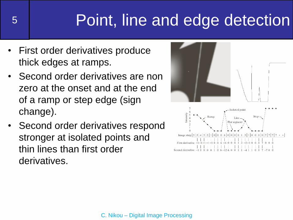
Point, line and edge detection
• First order derivatives produce
thick edges at ramps.
• Second order derivatives are non
zero at the onset and at the end
of a ramp or step edge (sign
change).
• Second order derivatives respond
stronger at isolated points and
thin lines than first order
derivatives.

6
C. Nikou – Digital Image Processing
Detection of isolated points
• Simple operation using the Laplacian.
21 if ( , )( , )
0 otherwise
f x y Tg x y

7
C. Nikou – Digital Image Processing
Line detection
• The Laplacian is
also used here.
• It has a double
response
– Positive and
negative values at
the beginning and
end of the edges.
• Lines should be thin
with respect to the
size of the detectorAbsolute value Positive value

8
C. Nikou – Digital Image Processing
Line detection (cont.)
• The Laplacian is isotropic.
• Direction dependent filters localize 1 pixel thick
lines at other orientations (0, 45, 90).

9
C. Nikou – Digital Image Processing
Line detection (cont.)
• The Laplacian is isotropic.
• Direction dependent filters
localize 1 pixel thick lines at
other orientations (0, 45, 90).
10
C. Nikou – Digital Image Processing
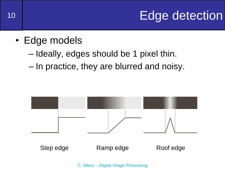
Edge detection
• Edge models
– Ideally, edges should be 1 pixel thin.
– In practice, they are blurred and noisy.
Step edge Ramp edge Roof edge

11
C. Nikou – Digital Image Processing
Edge detection (cont.)

12
C. Nikou – Digital Image Processing
Edge detection (cont.)
Edge point detection
• Magnitude of the first
derivative.
• Sign change of the second
derivative.
Observations:
• Second derivative produces
two values for an edge
(undesirable).
• Its zero crossings may be
used to locate the centres of
thick edges.
13
C. Nikou – Digital Image Processing
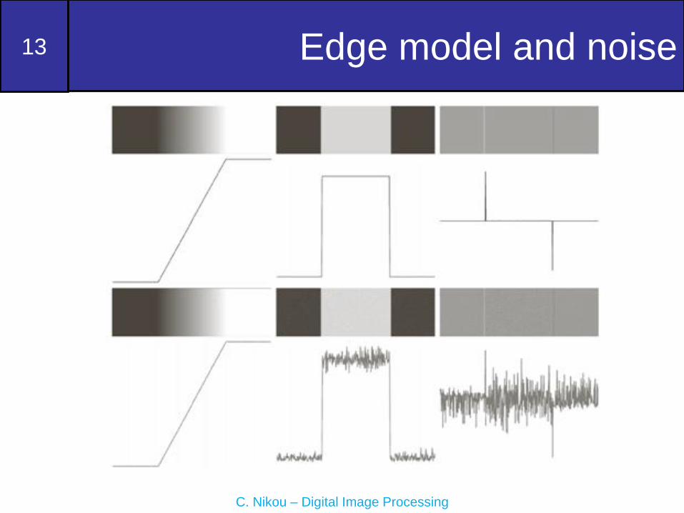
Edge model and noise

14
C. Nikou – Digital Image Processing
Edge model and noise (cont.)

15
C. Nikou – Digital Image Processing
Fundamental steps in edge
detection
• Image smoothing for noise reduction.
– Derivatives are very sensitive to noise.
• Detection of candidate edge points.
• Edge localization.
– Selection of the points that are true members
of the set of points comprising the edge.

16
C. Nikou – Digital Image Processing
The gradient points in the direction of most rapid increase
in intensity.
Image gradient
• The gradient of an image:
•
The gradient direction is given by
The edge strength is given by the gradient magnitude
Source: Steve Seitz

17
C. Nikou – Digital Image Processing
Gradient operators
( , )( 1, ) ( , )
f x yf x y f x y
x
( , )( , 1) ( , )
f x yf x y f x y
y
Roberts operators

18
C. Nikou – Digital Image Processing
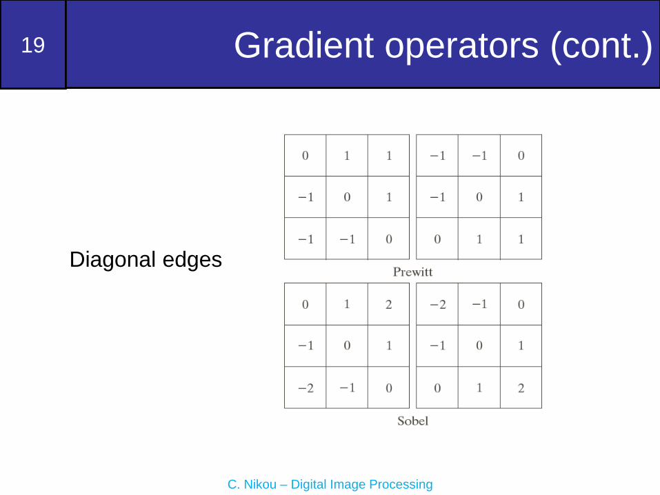
Gradient operators (cont.)
Integrates image
smoothing
19
C. Nikou – Digital Image Processing
Gradient operators (cont.)
Diagonal edges
20
C. Nikou – Digital Image Processing
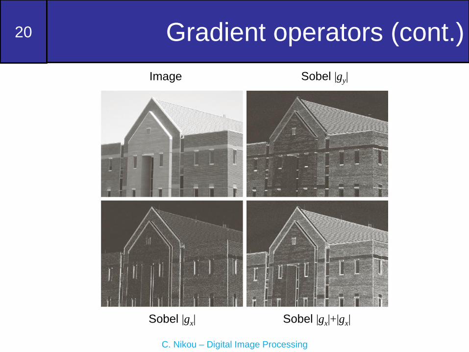
Gradient operators (cont.)
Image Sobel |gy|
Sobel |gx| Sobel |gx|+|gx|

21
C. Nikou – Digital Image Processing
Gradient operators (cont.)
Image smoothed
prior to edge
detection.
The wall bricks are
smoothed out.
Sobel |gy|
Sobel |gx| Sobel |gx|+|gx|
Image
22
C. Nikou – Digital Image Processing
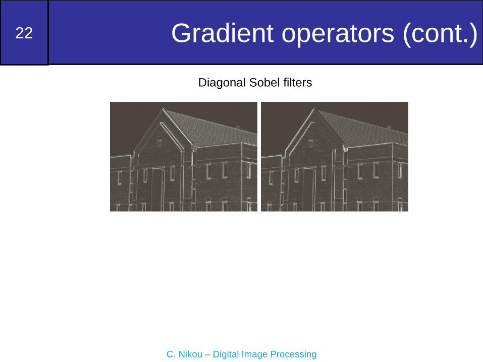
Gradient operators (cont.)
Diagonal Sobel filters

23
C. Nikou – Digital Image Processing
Gradient operators (cont.)
Thresholded Sobel gradient amplitydes at 33% of max value
Thresholded gradient Image smoothing prior to
gradient thresholding

24
C. Nikou – Digital Image Processing
The LoG operator
• A good place to look for edges is the maxima of the first
derivative or the zeros of the second derivative.
• The 2D extension approximates the second derivative by
the Laplacian operator (which is rotationally invariant):
2 22
2 2( , )
f ff x y
x y
• Marr and Hildreth [1980] argued that a satisfactory
operator that could be tuned in scale to detect edges is the
Laplacian of the Gaussian (LoG).

25
C. Nikou – Digital Image Processing
The LoG operator (cont.)
2 2( , )* ( , ) ( , )* ( , )G x y f x y G x y f x y
• The LoG operator is given by:
2 2 2 2
2 2
2 22
2 2
2 2 2 2 2
2 22 2 4
( , ) ( , )
2x y x y
G x y G x yx y
x ye e
x y
26
C. Nikou – Digital Image Processing
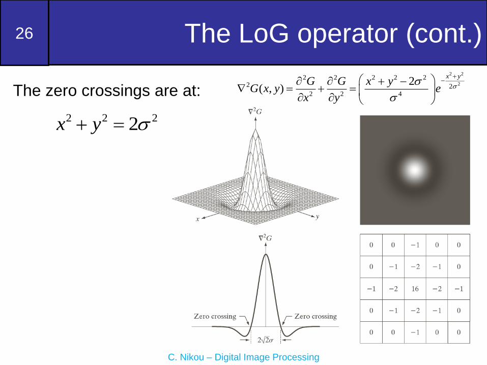
The LoG operator (cont.)
2 2
2
2 2 2 2 22 2
2 2 4
2( , )
x yG G x y
G x y ex y
The zero crossings are at:
2 2 22x y

27
C. Nikou – Digital Image Processing
The LoG operator (cont.)
• Fundamental ideas
– The Gaussian blurs the image. Iτ reduces the
intensity of structures at scales much smaller than σ.
– The Laplacian is isotropic and no other directional
mask is needed.
• The zero crossings of the operator indicate edge
pixels. They may be computed by using a 3x3
window around a pixel and detect if two of its
opposite neighbors have different signs (and
their difference is significant compared to a
threshold).

28
C. Nikou – Digital Image Processing
The LoG operator (cont.)
Image LoG
Zero
crossings
Zero crossings
with a threshold
of 4% of the
image max

29
C. Nikou – Digital Image Processing
The LoG operator (cont.)
• Filter the image at various scales and keep the zero
crossings that are common to all responses.
• Marr and Hildreth [1980] showed that LoG may be
approximated by a difference of Gaussinas (DOG):2 2 2 2
2 21 22 2
1 22 2
1 2
1 1DoG( , ) ,
2 2
x y x y
x y e e
• Certain channels of the human visual system are
selective with respect to orientation and frequency
and can be modeled by a DoG with a ratio of
standard deviations of 1.75.

30
C. Nikou – Digital Image Processing
The LoG operator (cont.)
• Meaningful comparison between LoG and
DoG may be obtained after selecting the
value of σ for LoG so that LoG has the same
zero crossings as DoG:
2 2 22 1 2 1
2 2 2
1 2 2
ln
• The two functions should also be scaled to
have the same value at the origin.

31
C. Nikou – Digital Image Processing
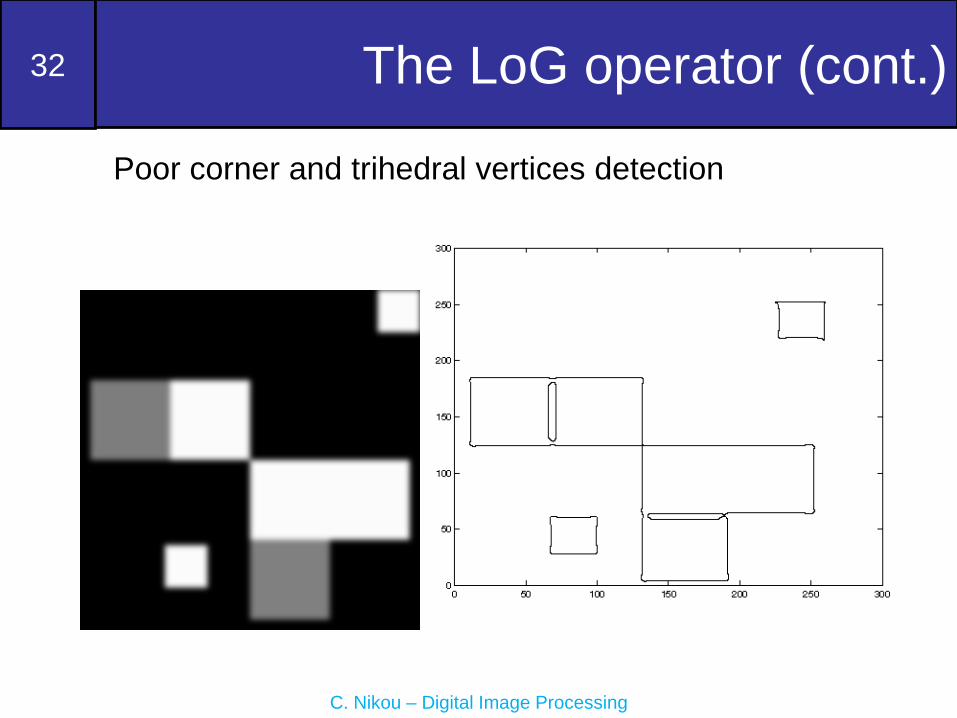
The LoG operator (cont.)
• LoG has fallen to some disfavour.
• It is not oriented and its response averages the
responses across the two directions.
– Poor response at corners.
– Difficulty in recording the topology of T-junctions
(trihedral vertices).
• Several studies showed that image components
along an edge contribute to the response of LoG to
noise but not to a true edge. Thus, zero crossings
may not lie exactly on an edge.
32
C. Nikou – Digital Image Processing
The LoG operator (cont.)
Poor corner and trihedral vertices detection

33
C. Nikou – Digital Image Processing
Designing an optimal edge detector
• Criteria for an “optimal” edge detector [Canny 1986]:
– Good detection: the optimal detector must minimize the probability of
false positives (detecting spurious edges caused by noise), as well as
that of false negatives (missing real edges).
– Good localization: the edges detected must be as close as possible to
the true edges
– Single response: the detector must return one point only for each true
edge point; that is, minimize the number of local maxima around the true
edge.

34
C. Nikou – Digital Image Processing
Canny edge detector
• Probably the most widely used edge detector.
• Theoretical model: step-edges corrupted by
additive Gaussian noise.
• Canny has shown that the first derivative of the
Gaussian closely approximates the operator that
optimizes the product of signal-to-noise ratio and
localization.
2 2
2 22 22
x xd x
e ex

35
C. Nikou – Digital Image Processing
Canny edge detector
• Generalization to 2D by applying the 1D operator in
the direction of the edge normal.
• However, the direction of the edge normal is
unknown beforehand and the 1D filter should be
applied in all possible directions.
• This task may be approximated by smoothing the
image with a circular 2D Gaussian, computing the
gradient magnitude and use the gradient angle to
estimate the edge strength.

36
C. Nikou – Digital Image Processing
Canny edge detector (cont.)
1. Filter image with derivative of Gaussian.
2. Find magnitude and orientation of
gradient.
3. Non-maximum suppression:
– Thin multi-pixel wide “ridges” down to single
pixel width.
4. Linking and thresholding (hysteresis):
– Define two thresholds: low and high
– Use the high threshold to start edge curves
and the low threshold to continue them.

37
C. Nikou – Digital Image Processing
Canny edge detector (cont.)
original image

38
C. Nikou – Digital Image Processing
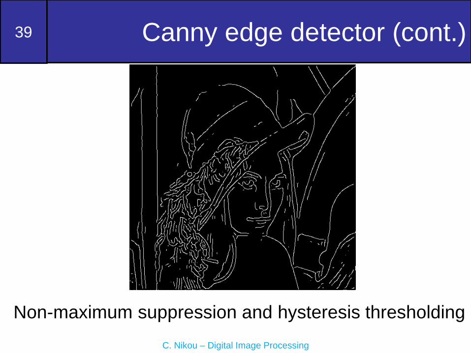
Canny edge detector (cont.)
Gradient magnitude
39
C. Nikou – Digital Image Processing
Canny edge detector (cont.)
Non-maximum suppression and hysteresis thresholding

40
C. Nikou – Digital Image Processing
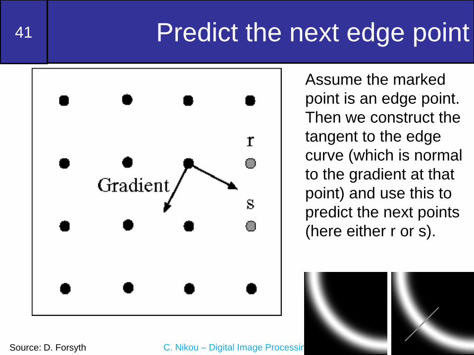
Non-maximum suppression (cont.)
At pixel q, we have a
maximum if the value of
the gradient magnitude
is larger than the values
at both p and at r.
Interpolation provides
these values.
Source: D. Forsyth
41
C. Nikou – Digital Image Processing
Assume the marked
point is an edge point.
Then we construct the
tangent to the edge
curve (which is normal
to the gradient at that
point) and use this to
predict the next points
(here either r or s).
Predict the next edge point
Source: D. Forsyth
42
C. Nikou – Digital Image Processing Source: S. Seitz
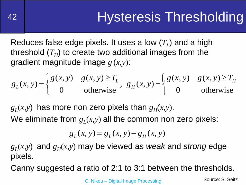
Reduces false edge pixels. It uses a low (TL) and a high
threshold (TH) to create two additional images from the
gradient magnitude image g (x,y):
Hysteresis Thresholding
( , ) ( , ) ( , ) ( , )( , ) , ( , )
0 otherwise 0 otherwise
L H
L H
g x y g x y T g x y g x y Tg x y g x y
gL(x,y) has more non zero pixels than gH(x,y).
We eliminate from gL(x,y) all the common non zero pixels:
( , ) ( , ) ( , )L L Hg x y g x y g x y
gL(x,y) and gH(x,y) may be viewed as weak and strong edge
pixels.
Canny suggested a ratio of 2:1 to 3:1 between the thresholds.

43
C. Nikou – Digital Image Processing Source: S. Seitz
• After the thresholdings, all strong pixels are
assumed to be valid edge pixels. Depending
on the value of TH, the edges in gH(x,y)
typically have gaps.
• All pixels in gL(x,y) are considered valid edge
pixels if they are 8-connected to a valid edge
pixel in gH(x,y).
Hysteresis Thresholding (cont.)

44
C. Nikou – Digital Image Processing
Hysteresis thresholding (cont.)
high threshold
(strong edges)
low threshold
(weak edges)
hysteresis threshold
Source: L. Fei-Fei
45
C. Nikou – Digital Image Processing
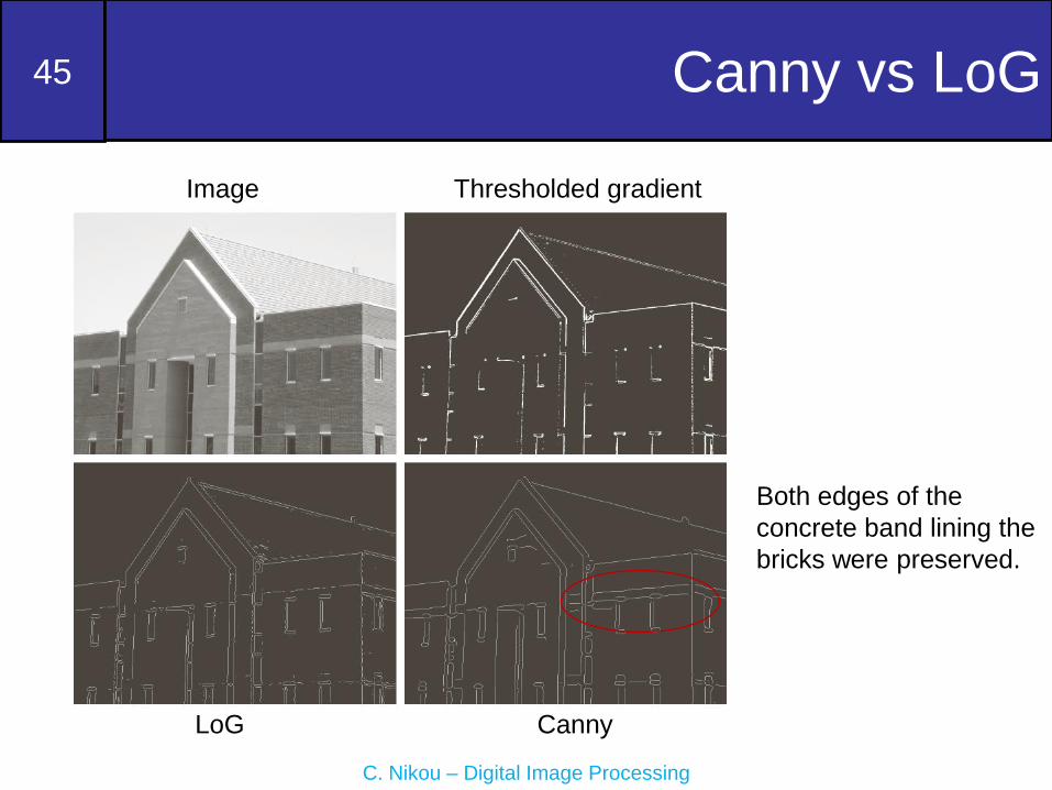
Canny vs LoG
Image
LoG Canny
Thresholded gradient
Both edges of the
concrete band lining the
bricks were preserved.
46
C. Nikou – Digital Image Processing
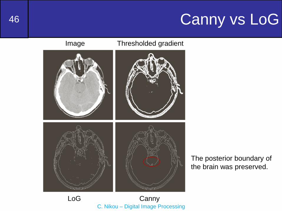
Canny vs LoG
Image
LoG Canny
Thresholded gradient
The posterior boundary of
the brain was preserved.
47
C. Nikou – Digital Image Processing
Edge Linking
• Even after hysteresis thresholding, the detected
pixels do not completely characterize edges
completely due to occlusions, non-uniform
illumination and noise. Edge linking may be:
– Local: requiring knowledge of edge points in
a small neighborhood.
– Regional: requiring knowledge of edge
points on the boundary of a region.
– Global: the Hough transform, involving the
entire edge image.

48
C. Nikou – Digital Image Processing
Edge Linking by Local Processing
A simple algorithm:
1. Compute the gradient magnitude and angle
arrays M(x,y) and a(x,y) of the input image f(x,y).
2. Let Sxy denote the neighborhood of pixel (x,y).
3. A pixel (s,t) in Sxy in is linked to (x,y) if:
( , ) ( , ) and ( , ) ( , )M x y M s t E a x y a s t A
A record of linked points must be kept as the
center of Sxy moves.
Computationally expensive as all neighbors of
every pixel should be examined.

49
C. Nikou – Digital Image Processing
Edge Linking by Local Processing
(cont.)A faster algorithm:
1. Compute the gradient magnitude and angle arrays
M(x,y) and a(x,y) of the input image f(x,y).
2. Form a binary image:
1 ( , ) and ( , ) [ , ]( , )
0 otherwise
M A AM x y T a x y A T A Tg x y
3. Scan the rows of g(x,y) (for Α=0) and fill (set to 1) all
gaps (zeros) that do not exceed a specified length K.
4. To detect gaps in any other direction Α=θ, rotate g(x,y)
by θ and apply the horizontal scanning.

50
C. Nikou – Digital Image Processing
Edge Linking by Local Processing
(cont.)Image Gradient magnitude Horizontal linking
Vertical linking Logical OR Morphological thinning
We may detect the
licence plate from the
ratio width/length (2:1 in
the USA)
51
C. Nikou – Digital Image Processing
Edge Linking by Regional
Processing
• Often, the location of regions of interest is known
and pixel membership to regions is available.
• Approximation of the region boundary by fitting a
polygon. Polygons are attractive because:
– They capture the essential shape.
– They keep the representation simple.
• Requirements
– Two starting points must be specified (e.g.
rightmost and leftmost points).
– The points must be ordered (e.g. clockwise).

52
C. Nikou – Digital Image Processing
Edge Linking by Regional
Processing (cont.)
• Variations of the algorithm handle both open and
closed curves.
• If this is not provided, it may be determined by
distance criteria:
– Uniform separation between points indicate a closed
curve.
– A relatively large distance between consecutive
points with respect to the distances between other
points indicate an open curve.
• We present here the basic mechanism for
polygon fitting.
53
C. Nikou – Digital Image Processing
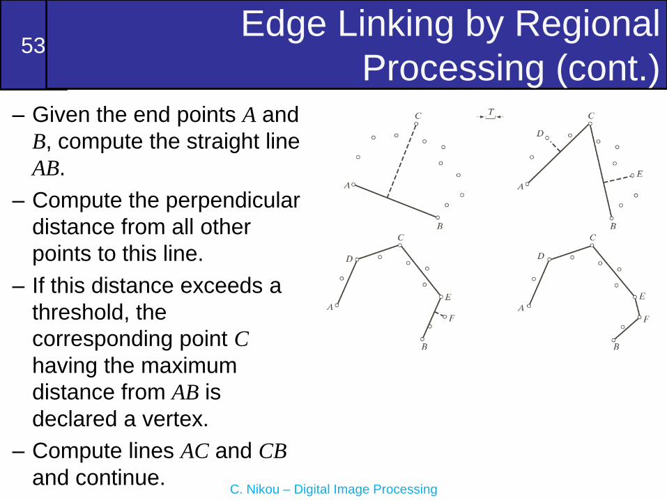
Edge Linking by Regional
Processing (cont.)– Given the end points A and
B, compute the straight line
AB.
– Compute the perpendicular
distance from all other
points to this line.
– If this distance exceeds a
threshold, the
corresponding point C
having the maximum
distance from AB is
declared a vertex.
– Compute lines AC and CB
and continue.

54
C. Nikou – Digital Image Processing
Edge Linking by Regional
Processing (cont.)Regional processing for edge linking is used in combination
with other methods in a chain of processing.

55
C. Nikou – Digital Image Processing
Hough transform
• An early type of voting scheme.
• Each line is defined by two points (xi,yi) and (xj,yj).
• Each point (xi,yi) has a line parameter space (a,b)
because it belongs to an infinite number of lines yi=axi+b.
• All the points (x,y) on a line y=a’x+b’ have lines in
parameter space that intersect at (a’x+b’).
Image space Parameter
space
56
C. Nikou – Digital Image Processing
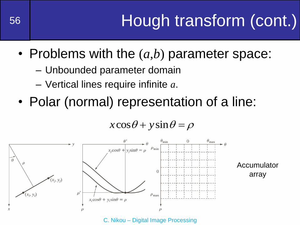
• Problems with the (a,b) parameter space:– Unbounded parameter domain
– Vertical lines require infinite a.
• Polar (normal) representation of a line:
Hough transform (cont.)
cos sinx y
Accumulator
array

57
C. Nikou – Digital Image Processing
Hough transform (cont.)
• A: intersection of curves corresponding to points 1, 3, 5.• B: intersection of curves corresponding to points 2, 3, 4.• Q, R and S show the reflective adjacency at the edges of
the parameter space. They do not correspond to points.

58
C. Nikou – Digital Image Processing
Hough transform (cont.)
• We only know the orientation of the runway (around 0 deg) and the observer’s position relative to it (GPS, flight charts etc.).
• We look for the peak at the accumulator array around 0 deg and join gaps below 20% of the image height.
• Applications in autonomous navigation.

59
C. Nikou – Digital Image Processing
Practical details
• Try to get rid of irrelevant features
– Take only edge points with significant gradient
magnitude.
• Choose a good grid / discretization
– Too coarse: large votes obtained when too many
different lines correspond to a single bucket.
– Too fine: miss lines because some points that are not
exactly collinear cast votes for different buckets.
• Increment also neighboring bins (smoothing in
accumulator array).

60
C. Nikou – Digital Image Processing
Thresholding
• Image partitioning into regions directly
from their intensity values.
1 if ( , )( , )
0 if ( , )
f x y Tg x y
f x y T
1
1 2
2
0 if ( , )
( , ) 1 if ( , )
2 if ( , )
f x y T
g x y T f x y T
f x y T

61
C. Nikou – Digital Image Processing
Noise in Thresholding
Noiseless Gaussian (μ=0, σ=10) Gaussian (μ=0, σ=10)
Difficulty in determining the threshold due to noise

62
C. Nikou – Digital Image Processing
Illumination in Thresholding
(a) Noisy image (b) Intensity ramp
image
Multiplication
Difficulty in determining the threshold due to non-uniform illumination

63
C. Nikou – Digital Image Processing
Basic Global Thresholding
• Algorithm
– Select initial threshold estimate T.
– Segment the image using T
• Region G1 (values > T) and region G2 (values < T).
– Compute the average intensities m1 and m2 of
regions G1 and G2 respectively.
– Set T=(m1+m2)/2
– Repeat until the change of T in successive
iterations is less than ΔΤ.

64
C. Nikou – Digital Image Processing
Basic Global Thresholding (cont.)
T=125

65
C. Nikou – Digital Image Processing
Optimum Global Thresholding
using Otsu’s Method• The method is based on statistical decision theory.
• Minimization of the average error of assignment of pixels
to two (or more) classes.
• Bayes decision rule may have a nice closed form solution
to this problem provided
– The pdf of each class.
– The probability of class occurence.
• Pdf estimation is not trivial and assumptions are made
(Gaussian pdfs).
• Otsu (1979) proposed an attractive alternative maximizing
the between-class variance.
– Only the histogram of the image is used.

66
C. Nikou – Digital Image Processing
Otsu’s Method (cont.)
• Let {0, 1, 2,…, L-1} denote the intensities of a
MxN image and ni the number of pixels with
intensity i.
• The normalized histogram has components:1
0
, 1, 0L
ii i i
i
np p p
MN
• Suppose we choose a threshold k to segment the
image into two classes:
• C1 with intensities in the range [0, k],
• C2 with intensities in the range [k+1, L-1].

67
C. Nikou – Digital Image Processing
Otsu’s Method (cont.)
• The probabilities of classes C1 and C2:
1
1 2 1
0 1
( ) , ( ) 1 ( )k L
i i
i i k
P k p P k p P k
• The mean intensity of class C1 :
11 1
0 0 01 1
( | ) ( ) 1( ) ( | )
( ) ( )
k k k
i
i i i
P C i P im k iP i C i ip
P C P k
1( | ) 1P C i Intensity i belongs to class C1 and

68
C. Nikou – Digital Image Processing
Otsu’s Method (cont.)
• Similarly, the mean intensity of class C2:1 1 1
22 2
1 1 12 2
( | ) ( ) 1( ) ( | )
( ) ( )
L L L
i
i k i k i k
P C i P im k iP i C i ip
P C P k
• Mean image intensity:1
1 1 2 2
0
( ) ( ) ( ) ( )L
G i
i
m ip P k m k P k m k
• Cumulative mean image intensity (up to k):
0
( )k
i
i
m k ip
69
C. Nikou – Digital Image Processing
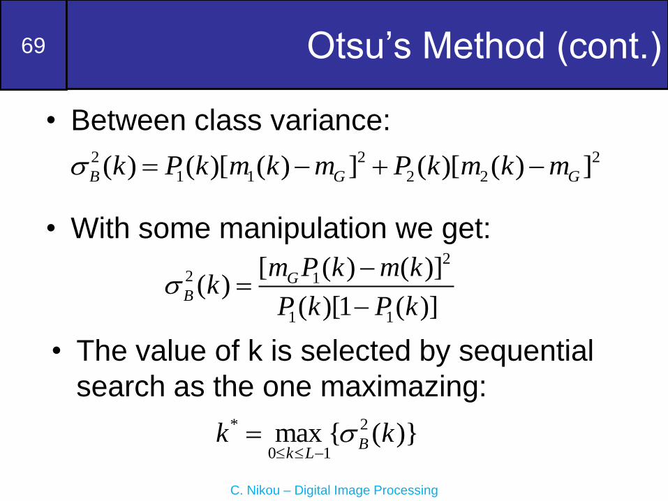
Otsu’s Method (cont.)
• Between class variance:2 2 2
1 1 2 2( ) ( )[ ( ) ] ( )[ ( ) ]B G Gk P k m k m P k m k m
• With some manipulation we get:2
2 1
1 1
[ ( ) ( )]( )
( )[1 ( )]
GB
m P k m kk
P k P k
• The value of k is selected by sequential
search as the one maximazing:* 2
0 1max { ( )}B
k Lk k
70
C. Nikou – Digital Image Processing
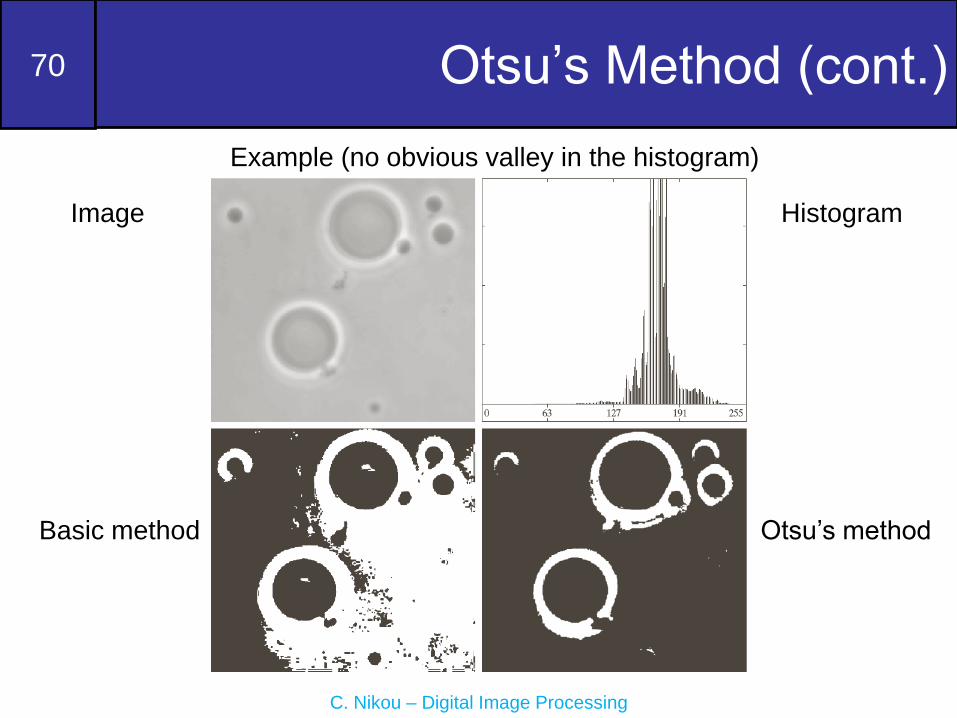
Otsu’s Method (cont.)
Basic method
Example (no obvious valley in the histogram)
Image Histogram
Otsu’s method
71
C. Nikou – Digital Image Processing
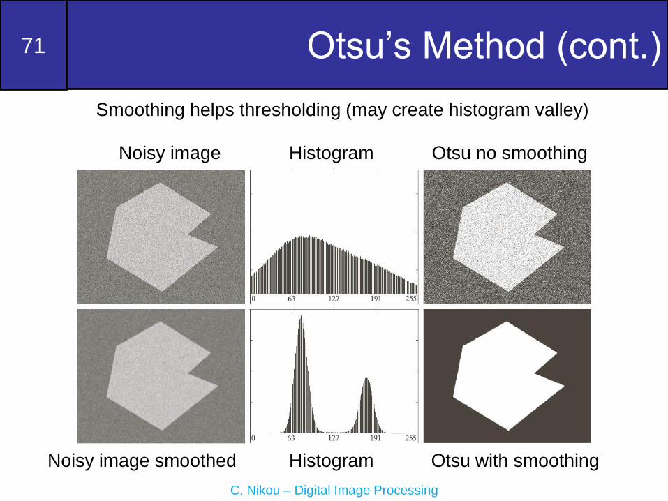
Otsu’s Method (cont.)
Noisy image smoothed
Smoothing helps thresholding (may create histogram valley)
Noisy image Histogram
Otsu with smoothing
Otsu no smoothing
Histogram

72
C. Nikou – Digital Image Processing
Otsu’s Method (cont.)
Noisy image smoothed
Otsu’s method, even with smoothing cannot extract small structures
Noisy image, σ=10 Histogram
Otsu with smoothing
Otsu no smoothing
Histogram

73
C. Nikou – Digital Image Processing
Otsu’s Method (cont.)
• Dealing with small structures
– The histogram is unbalanced• The background dominates
• No valleys indicating the small structure.
– Idea: consider only the pixels around edges• Both structure of interest and background are present equally.
• More balanced histograms
– Use gradient magnitude or zero crossings of
the Laplacian.
• Threshold it at a percentage of the maximum value.
• Use it as a mask on the original image.
• Only pixels around edges will be employed.

74
C. Nikou – Digital Image Processing
Otsu’s Method (cont.)
Multiplication
(Mask x Image)
Noisy image, σ=10 Histogram
Otsu
Gradient magnitude
mask (at 99.7% of max)
Histogram
75
C. Nikou – Digital Image Processing
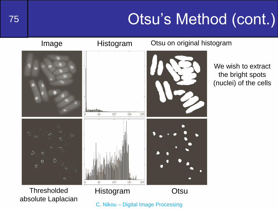
Otsu’s Method (cont.)
Image Histogram Otsu on original histogram
Thresholded
absolute LaplacianOtsuHistogram
We wish to extract
the bright spots
(nuclei) of the cells

76
C. Nikou – Digital Image Processing
Otsu’s Method (cont.)
• The method may be extended to multiple thresholds
• In practice for more than 2 thresholds (3 segments)
more advanced methods are employed.
• For three classes, the between-class variance is:
2
1 2 1 1 1 1 2 1 2 2 1 2 3 2 3 2( , ) ( )[ ( ) ] ( , )[ ( , ) ] ( )[ ( ) ]B G G Gk k P k m k m P k k m k k m P k m k m
• The thresholds are computed by searching all
pairs for values:
1 2
* * 2
1 2 1 20 1
( , ) max { ( , )}Bk k L
k k k k

77
C. Nikou – Digital Image Processing
Otsu’s Method (cont.)
Image of iceberg segmented into three regions.
k1=80, k2=177

78
C. Nikou – Digital Image Processing
Variable Thresholding
Otsu
Image partitioning.
The image is sub-divided and the method is applied to every sub-image.
Useful for illumination non-uniformity correction.
Shaded image Histogram
Otsu at each sub-image
Simple thresholding
Subdivision

79
C. Nikou – Digital Image Processing
Variable Thresholding(cont.)
Use of local image properties.
• Compute a threshold for every single pixel in the image
based on its neighborhood (mxy, σxy,…).
1 (localproperties) is true( , )
0 (localproperties) is false
Qg x y
Q
true ( , ) ( , )( , )
false otherwise
xy xy
xy xy
f x y a AND f x y bmQ m

80
C. Nikou – Digital Image Processing
Variable Thresholding (cont.)
Image of local
standard deviations
Image
Histogram
Local
Thresholding
More accurate
nuclei extraction.
Otsu with
2 thresholds
Subdivision
81
C. Nikou – Digital Image Processing
Variable Thresholding (cont.)
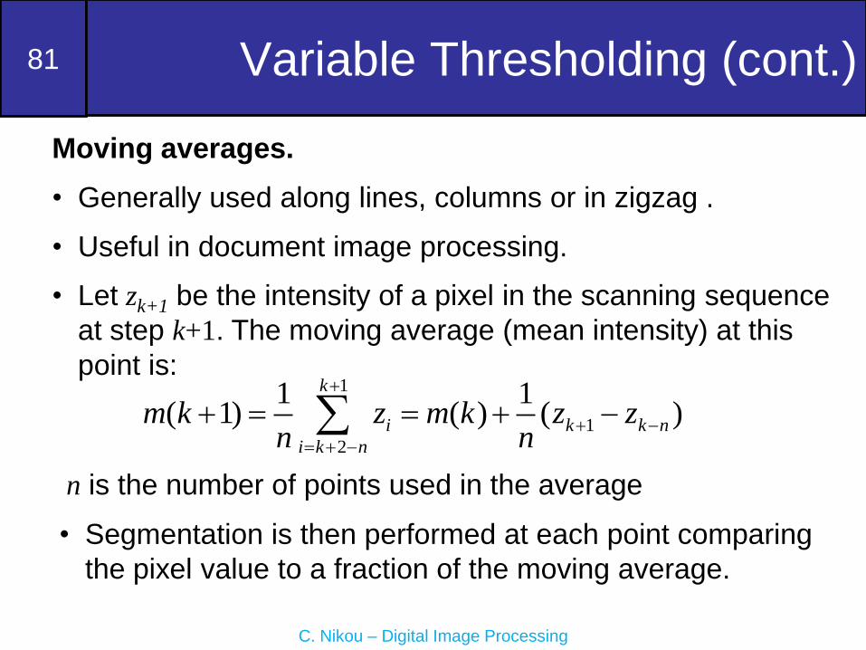
Moving averages.
• Generally used along lines, columns or in zigzag .
• Useful in document image processing.
• Let zk+1 be the intensity of a pixel in the scanning sequence
at step k+1. The moving average (mean intensity) at this
point is:1
1
2
1 1( 1) ( ) ( )
k
i k k n
i k n
m k z m k z zn n
n is the number of points used in the average
• Segmentation is then performed at each point comparing
the pixel value to a fraction of the moving average.

82
C. Nikou – Digital Image Processing
Variable Thresholding (cont.)
Shaded text images
occur typically from
photographic flashes
Otsu Moving averages

83
C. Nikou – Digital Image Processing
Variable Thresholding (cont.)
Sinusoidal variations (the
power supply of the scanner
not grounded properly)
Otsu Moving averages
The moving average works well when the structure of interest is
small with respect to image size (handwritten text).

84
C. Nikou – Digital Image Processing
Region Growing
• Start with seed points S(x,y) and grow to larger
regions satisfying a predicate.
• Needs a stopping rule.
• Algorithm
– Find all connected components in S(x,y) and erode
them to 1 pixel.
– Form image fq(x,y)=1 if f (x,y) satisfies the predicate.
– Form image g(x,y)=1 for all pixels in fq(x,y) that are 8-
connected with to any seed point in S(x,y).
– Label each connected component in g(x,y) with a
different label.

85
C. Nikou – Digital Image Processing
Region Growing (cont.)
X-Ray image of weld
with a crack we want to
segment.
Histogram Seed image (99.9% of
max value in the initial
image).
Crack pixels are missing.
The weld is very bright. The predicate used for region growing is to
compare the absolute difference between a seed point and a pixel
to a threshold. If the difference is below it we accept the pixel as
crack.

86
C. Nikou – Digital Image Processing
Region Growing (cont.)
Seed image eroded to 1
pixel regions.
Difference between
the original image and
the initial seed image.
The pixels are ready
to be compared to the
threshold.
Histogram of the
difference image.
Two valleys at 68
and 126 provided
by Otsu.
87
C. Nikou – Digital Image Processing
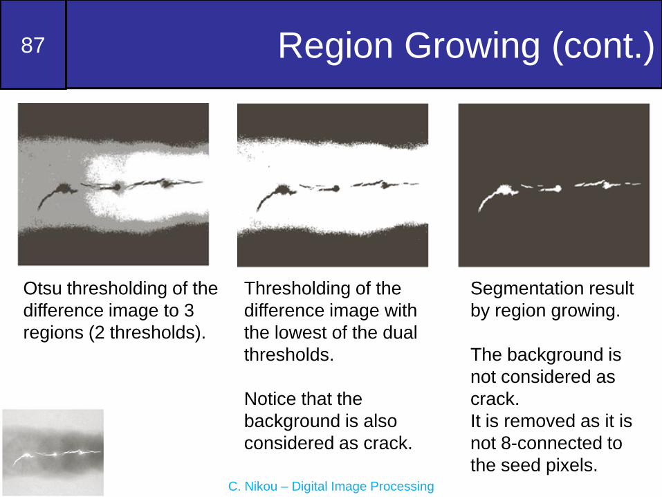
Region Growing (cont.)
Otsu thresholding of the
difference image to 3
regions (2 thresholds).
Thresholding of the
difference image with
the lowest of the dual
thresholds.
Notice that the
background is also
considered as crack.
Segmentation result
by region growing.
The background is
not considered as
crack.
It is removed as it is
not 8-connected to
the seed pixels.

88
C. Nikou – Digital Image Processing
Region Splitting and Merging
• Based on quadtrees (quadimages).
• The root of the tree corresponds to the image.
• Split the image to sub-images that do not satisfy
a predicate Q.
• If only splitting was used, the final partition would
contain adjacent regions with identical
properties.
• A merging step follows merging regions
satisfying the predicate Q.

89
C. Nikou – Digital Image Processing
Region Splitting and Merging
(cont.)• Algorithm
– Split into four disjoint quadrants any region Ri for
which Q(Ri)=FALSE.
– When no further splitting is possible, merge any
adjacent regions Ri and Rk for which Q(Ri Rk)=TRUE.
– Stop when no further merging is possible.
• A maximum quadregion size is specified beyond which no
further splitting is carried out.
• Many variations heve been proposed.
– Merge any adjacent regions if each one satisfies the
predicate individually (even if their union does not
satisfy it).

90
C. Nikou – Digital Image Processing
Region Splitting and Merging
(cont.)
Merging examples:
• R2 may be merged with R41.
• R41 may be merged with R42.
Quadregions resulted from splitting.
91
C. Nikou – Digital Image Processing
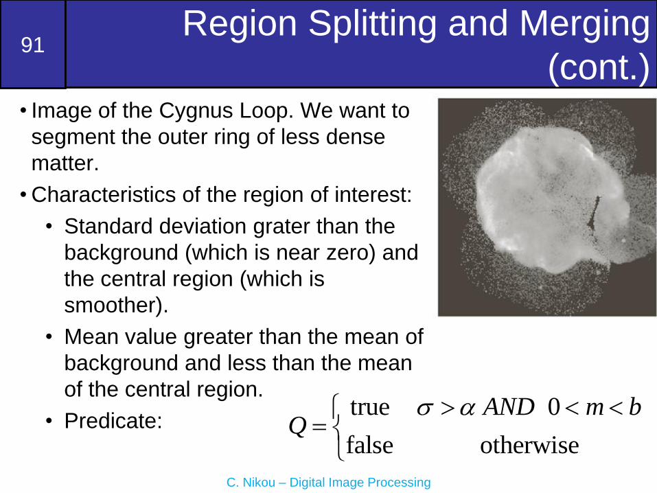
Region Splitting and Merging
(cont.)• Image of the Cygnus Loop. We want to
segment the outer ring of less dense
matter.
• Characteristics of the region of interest:
• Standard deviation grater than the
background (which is near zero) and
the central region (which is
smoother).
• Mean value greater than the mean of
background and less than the mean
of the central region.
• Predicate:true 0
false otherwise
AND m bQ

92
C. Nikou – Digital Image Processing
Region Splitting and Merging
(cont.)Varying the size of the smallest allowed quadregion.
32x32
16x16 8x8
Larger quadregions
lead to block-like
segmentation.
Smaller quadregions
lead to small black
regions.
16x16 seems to be
the best result.
93
C. Nikou – Digital Image Processing
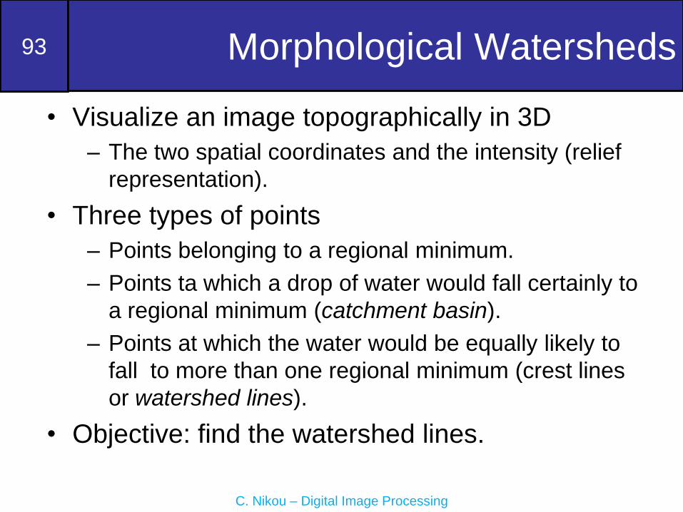
Morphological Watersheds
• Visualize an image topographically in 3D
– The two spatial coordinates and the intensity (relief
representation).
• Three types of points
– Points belonging to a regional minimum.
– Points ta which a drop of water would fall certainly to
a regional minimum (catchment basin).
– Points at which the water would be equally likely to
fall to more than one regional minimum (crest lines
or watershed lines).
• Objective: find the watershed lines.
94
C. Nikou – Digital Image Processing
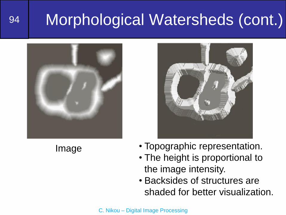
Morphological Watersheds (cont.)
Image • Topographic representation.
• The height is proportional to
the image intensity.
• Backsides of structures are
shaded for better visualization.

95
C. Nikou – Digital Image Processing
Morphological Watersheds (cont.)
• A hole is punched in each regional minimum and the topography is
flooded by water from below through the holes.
• When the rising water is about to merge in catchment basins, a dam is
built to prevent merging.
• There will be a stage where only the tops of the dams will be visible.
• These continuous and connected boundaries are the result of the
segmentation.

96
C. Nikou – Digital Image Processing
Morphological Watersheds (cont.)
• Topographic representation of the image.
• A hole is punched in each regional minimum (dark
areas) and the topography is flooded by water (at
equal rate) from below through the holes.
Regional
minima

97
C. Nikou – Digital Image Processing
Morphological Watersheds (cont.)
• Before flooding.
• To prevent water from spilling through the image
borders, we consider that the image is surrounded
by dams of height greater than the maximum image
intensity.

98
C. Nikou – Digital Image Processing
Morphological Watersheds (cont.)
• First stage of flooding.
• The water covered areas corresponding to the dark
background.

99
C. Nikou – Digital Image Processing
Morphological Watersheds (cont.)
• Next stages of flooding.
• The water has risen into the other catchment basin.

100
C. Nikou – Digital Image Processing
Morphological Watersheds (cont.)
• Further flooding. The water has risen into the third
catchment basin.
101
C. Nikou – Digital Image Processing
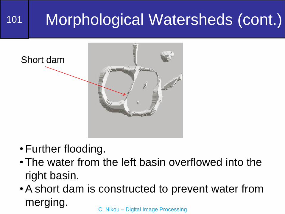
Morphological Watersheds (cont.)
• Further flooding.
• The water from the left basin overflowed into the
right basin.
• A short dam is constructed to prevent water from
merging.
Short dam
102
C. Nikou – Digital Image Processing
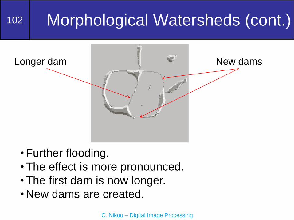
Morphological Watersheds (cont.)
• Further flooding.
• The effect is more pronounced.
• The first dam is now longer.
• New dams are created.
Longer dam New dams
103
C. Nikou – Digital Image Processing
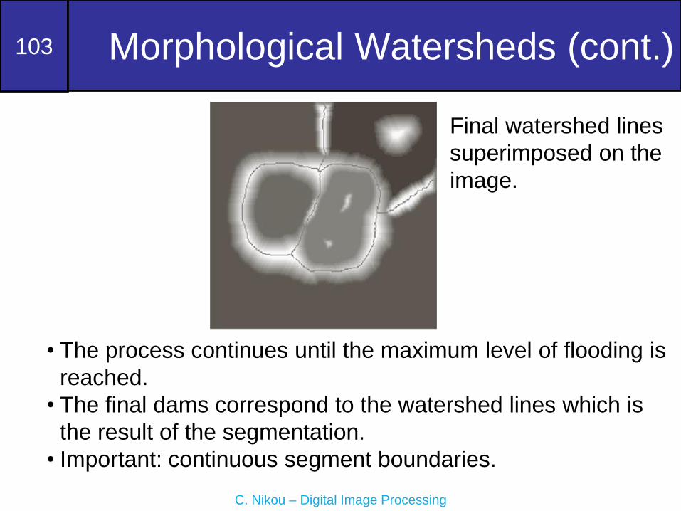
Morphological Watersheds (cont.)
• The process continues until the maximum level of flooding is
reached.
• The final dams correspond to the watershed lines which is
the result of the segmentation.
• Important: continuous segment boundaries.
Final watershed lines
superimposed on the
image.

104
C. Nikou – Digital Image Processing
Morphological Watersheds (cont.)
• Dams are constructed by morphological dilation.
Flooding step n-1.
Regional minima: M1 and M2.
Catchment basins associated: Cn-1(M1) and Cn-1(M2).
Cn-1(M1) Cn-1(M2)
1 1 1 2[ 1] ( ) ( )n nC n C M C M
C[n-1] has two connected components.

105
C. Nikou – Digital Image Processing
Morphological Watersheds (cont.)
Flooding step n-1. Flooding step n.
Cn-1(M1) Cn-1(M2)
• If we continue flooding, then we will have one connected
component.
• This indicates that a dam must be constructed.
• Let q be the merged connected component if we perform
flooding a step n.
q
106
C. Nikou – Digital Image Processing
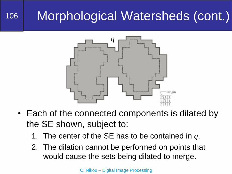
Morphological Watersheds (cont.)
• Each of the connected components is dilated by
the SE shown, subject to:
1. The center of the SE has to be contained in q.
2. The dilation cannot be performed on points that
would cause the sets being dilated to merge.
q

107
C. Nikou – Digital Image Processing
Morphological Watersheds (cont.)
• In the first dilation, condition 1 was satisfied by every
point and condition 2 did not apply to any point.
• In the second dilation, several points failed condition 1
while meeting condition 2 (the points in the perimeter
which is broken).
Conditions
1. Center of SE in q.
2. No dilation if merging.

108
C. Nikou – Digital Image Processing
Morphological Watersheds (cont.)
• The only points in q that satisfied both conditions form
the 1-pixel thick path.
• This is the dam at step n of the flooding process.
• The points should satisfy both conditions.
Conditions
1. Center of SE in q.
2. No dilation if merging.

109
C. Nikou – Digital Image Processing
Morphological Watersheds (cont.)
• A common application
is the extraction of
nearly uniform, blob-
like objects from their
background.
• For this reason it is
generally applied to the
gradient of the image
and the catchment
basins correspond to
the blob like objects.
Image Gradient magnitude
Watersheds Watersheds
on the image

110
C. Nikou – Digital Image Processing
Morphological Watersheds (cont.)
• Noise and local minima lead generally to oversegmentation.
• The result is not useful.
• Solution: limit the number of allowable regions by additional
knowledge.

111
C. Nikou – Digital Image Processing
Morphological Watersheds (cont.)
• Markers (connected components):
– internal, associated with the objects
– external, associated with the background.
• Here the problem is the large number of local
minima.
• Smoothing may eliminate them.
• Define an internal marker (after smoothing):
• Region surrounded by points of higher
altitude.
– They form connected components.
– All points in the connected component have the
same intensity.
112
C. Nikou – Digital Image Processing
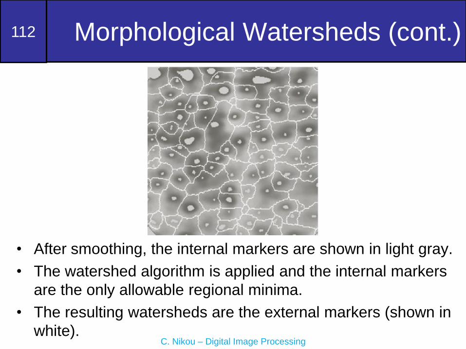
Morphological Watersheds (cont.)
• After smoothing, the internal markers are shown in light gray.
• The watershed algorithm is applied and the internal markers
are the only allowable regional minima.
• The resulting watersheds are the external markers (shown in
white).

113
C. Nikou – Digital Image Processing
Morphological Watersheds (cont.)
• Each region defined by the external marker has a single internal marker
and part of the background.
• The problem is to segment each of these regions into two segments: a
single object and background.
• The algorithms we saw in this lecture may be used (including watersheds
applied to each individual region).
114
C. Nikou – Digital Image Processing
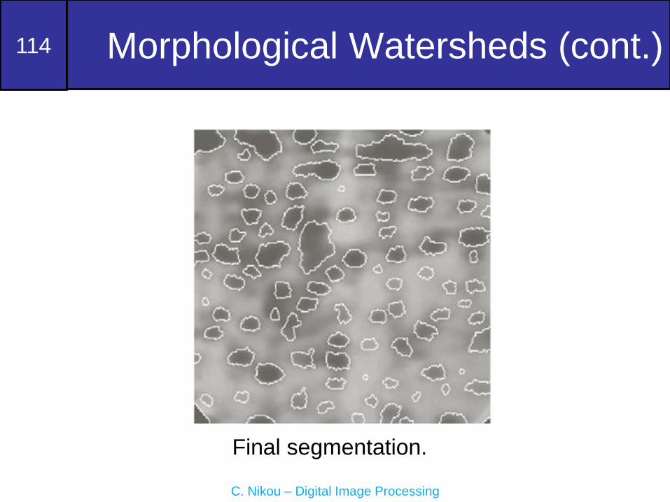
Morphological Watersheds (cont.)
Final segmentation.

115
C. Nikou – Digital Image Processing
Morphological Watersheds (cont.)
Image Watersheds Watersheds with markers

116
C. Nikou – Digital Image Processing
The use of motion in segmentation
• Powerful cue used by humans to extract
objects and regions.
• Motion arises from
– Objects moving in the scene.
– Relative displacement between the sensing
system and the scene (e.g. robotic
applications, autonomous navigation).
• We will consider motion
– Spatially.
– In the frequency domain.

117
C. Nikou – Digital Image Processing
Basic spatial motion segmentation
• Difference image and comparison with
respect to a threshold:
1 if ( , , ) ( , , )( , )
0 otherwise
i j
ij
f x y t f x y t Td x y
• The images should be registered.
• Illumination should be relatively constant
within the bounds defined by T.

118
C. Nikou – Digital Image Processing
Accumulative differences
• Comparison of a reference image with every
subsequent image in the sequence.
• A counter is incremented every time a pixel in
the current image is different from the reference
image.
• When the kth frame is being examined, the entry
in a given pixel of the accumulative difference
image (ADI) gives the number of times this pixel
differs from its counterpart in the reference
image.

119
C. Nikou – Digital Image Processing
Accumulative differences (cont.)
• Absolute ADI:
1
1
( , ) 1 if ( , ) ( , , )( , )
( , ) otherwise
k k
k
k
A x y R x y f x y t TA x y
A x y
• Positive ADI:
1
1
( , ) 1 if ( , ) ( , , )( , )
( , ) otherwise
k k
k
k
P x y R x y f x y t TP x y
P x y
• Negative ADI:
1
1
( , ) 1 if ( , ) ( , , )( , )
( , ) otherwise
k k
k
k
N x y R x y f x y t TN x y
N x y

120
C. Nikou – Digital Image Processing
Accumulative differences (cont.)
• ADIs for a rectangular object moving to southeast.
Absolute Positive Negative
• The nonzero area of the positive ADI gives the size of the object.
• The location of the positive ADI gives the location of the object in the
reference frame.
• The direction and speed may be obtained fom the absolute and
negative ADIs.
• The absolute ADI contains both the positive and negative ADIs.
121
C. Nikou – Digital Image Processing
Accumulative differences (cont.)
• To establish a reference image in a non
stationary background.
– Consider the first image as the reference image.
– When a non stationary component has moved out of
its position in the reference frame, the corresponding
background in the current frame may be duplicated
in the reference frame. This is determined by the
positive ADI:
• When the moving object is displaced completely with
respect to the reference frame the positive ADI stops
increasing.

122
C. Nikou – Digital Image Processing
Accumulative differences (cont.)
• Subtraction of the car going from left to right to
establish a reference image.
• Repeating the task for all moving objects may
result in a static reference image.
• The method works well only in simple scenarios.
123
C. Nikou – Digital Image Processing
Frequency domain techniques
• Consider a sequence f (x,y,t), t=0,1,…,K-1 of size M x N.
• All frames have an homogeneous zero background
except of a single pixel object with intensity of 1 moving
with constant velocity.
• At time t=0, the object is at (x’, y’) and the image plane is
projected onto the vertical (x) axis. This results in a 1D
signal which is zero except at x’.
• If we multiply the 1D signal by exp[j2πα1xΔt], for
x=0,1,…,M-1 and sum the results we obtain the single
term exp[j2πα1x’Δt].
• In frame t=1, suppose that the object moved to (x’+1, y’),
that is, it has moved 1 pixel parallel to the x-axis. The
same procedure yields exp[j2πα1(x’+1)+Δt].

124
C. Nikou – Digital Image Processing
Frequency domain techniques
(cont.)• Applying Euler’s formula, for t=0,1,…,K-1:
12 ( )
1 1cos[2 ( ) ] sin[2 ( ) ]j x t te x t t j x t t
• This is a complex exponential with frequency α1.
• If the object were moving V1 pixels (in the x-
direction) between frames the frequency would
have been V1α1.
• This causes the DFT of the 1D signal to have wo
peaks, one at V1α1 and one at K-V1α1.
• Division by a1 yields the velocity V1.
• These concepts may be generalized as follows.

125
C. Nikou – Digital Image Processing
Frequency domain techniques
(cont.)• For a sequence of K images of size M x N, the
sum of the weighted projections onto the x-axis
at an integer instant of time is:
1
1 12
1
0 0
( , ) ( , , ) , 0,1,..., 1M N
j x t
x
x y
g t f x y t e t K
• Similarly, the sum of the weighted projections
onto the y-axis at an integer instant of time is:
2
1 12
2
0 0
( , ) ( , , ) , 0,1,..., 1M N
j y t
y
x y
g t f x y t e t K
126
C. Nikou – Digital Image Processing
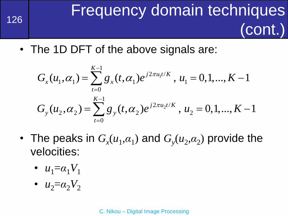
Frequency domain techniques
(cont.)• The 1D DFT of the above signals are:
1
12 /
1 1 1 1
0
( , ) ( , ) , 0,1,..., 1K
j u t K
x x
t
G u g t e u K
• The peaks in Gx(u1,α1) and Gy(u2,α2) provide the
velocities:
• u1=α1V1
• u2=α2V2
2
12 /
2 2 2 2
0
( , ) ( , ) , 0,1,..., 1K
j u t K
y y
t
G u g t e u K

127
C. Nikou – Digital Image Processing
Frequency domain techniques
(cont.)• The unit of velocity is in pixels per total frame
rate. For example, V1=10 is interpreted as a
motion of 10 pixels in K frames.
• For frames taken uniformly, the actual physical
speed depends on the frame rate and the
distance between pixels. Thus, for V1=10, K=30,
if the frame rate is two images/sec and the
distance between pixels is 0.5 m, the speed is:
– V1=(10 pixels)(0.5 m/pixel)(2 frames/sec) / (30 frames) =
1/3 m/sec.

128
C. Nikou – Digital Image Processing
Frequency domain techniques
(cont.)• The sign of the x-component of the velocity is
obtained by using Fourier properties of sinusoids:
2
1
1 2
Re ( , )x
x
t n
d g tS
dt
2
1
2 2
Im ( , )x
x
t n
d g tS
dt
• The above quantities will have the same sign at
an arbitrary time point t=n, if V1>0.
• Conversely, they will have opposite signs if V1<0.
• In practice, if either is zero, we consider the next
closest point.