linear methods for image compression - math 420, prof....

Linear Methods forImage

Compression

Aidan Meacham

Preliminaries

Color Spaces

Lossy vs. Lossless

Methods

SVD

PCA

DCT

Linear Methods for Image CompressionMath 420, Prof. Beezer

Aidan Meacham

University of Puget Sound


Compression

Aidan Meacham

Preliminaries

Color Spaces

Lossy vs. Lossless

Methods

SVD

PCA

DCT

Outline

PreliminariesColor SpacesLossy vs. Lossless

MethodsSVDPCADCT


Compression

Aidan Meacham

Preliminaries

Color Spaces

Lossy vs. Lossless

Methods

SVD

PCA

DCT

RGB Color Space

I Intensity and Representation

I Gamut mapping and Translation

I Absolute Color Spaces


Compression

Aidan Meacham

Preliminaries

Color Spaces

Lossy vs. Lossless

Methods

SVD

PCA

DCT

Lossy vs. Lossless Methods

I Lossless Methods - GIF / LZW

I Usefulness of Lossy Compression

I Limit - arithmetic, entropy, and LZW coding


Compression

Aidan Meacham

Preliminaries

Color Spaces

Lossy vs. Lossless

Methods

SVD

PCA

DCT

Outline

PreliminariesColor SpacesLossy vs. Lossless

MethodsSVDPCADCT


Compression

Aidan Meacham

Preliminaries

Color Spaces

Lossy vs. Lossless

Methods

SVD

PCA

DCT

SVD

Definition

I A is a matrix with singular values√σ1,√σ2, . . . ,

√σr ,

where r is the rank of A∗A and σi are eigenvalues of A

I Define V = [x1|x2| . . . |xn], U = [y1|y2| . . . |yn] where{xi} is an orthonormal basis of eigenvectors for A∗Aand yi = 1√

σiAxi


Compression

Aidan Meacham

Preliminaries

Color Spaces

Lossy vs. Lossless

Methods

SVD

PCA

DCT

SVD

I Additionally, si =√σi

I

S =

s1

s2 0. . .

sr

0 0. . .

0|0

I Thus,

AV = US

A = USV ∗


Compression

Aidan Meacham

Preliminaries

Color Spaces

Lossy vs. Lossless

Methods

SVD

PCA

DCT

SVD Truncated Form

I A =r∑

i=1sixiy

∗i , where r is the rank of A∗A and the si

are ordered in decreasing magnitude, s1 ≥ s2 ≥ · · · ≥ srI For i < r , this neglects the lower weighted singular

values

I Discarding unnecessary singular values and thecorresponding columns of U and V decreases theamount of storage necessary to reconstruct the image


Compression

Aidan Meacham

Preliminaries

Color Spaces

Lossy vs. Lossless

Methods

SVD

PCA

DCT

SVD ExampleSage

I Import image and convert to Sage matrix

I Perform SVD decomposition

I Choose number of singular values and reconstruct


Compression

Aidan Meacham

Preliminaries

Color Spaces

Lossy vs. Lossless

Methods

SVD

PCA

DCT

SVD Results

Cameraman, 256 elements Cameraman, 128 elements


Compression

Aidan Meacham

Preliminaries

Color Spaces

Lossy vs. Lossless

Methods

SVD

PCA

DCT

SVD Results



Compression

Aidan Meacham

Preliminaries

Color Spaces

Lossy vs. Lossless

Methods

SVD

PCA

DCT

Principal Component Analysis

I Wide variety of applications in many fields:I Principal moments and axes of inertia in physicsI Karhunen-Loeve Transform in signal processingI Predictive analytics - customer behavior

I Statistical method for maximizing “variance” of avariable; similar to SVD


Compression

Aidan Meacham

Preliminaries

Color Spaces

Lossy vs. Lossless

Methods

SVD

PCA

DCT

Statistics / Information Theory

I Variables with greater variance (higher entropy) carrymore information

I Maximizing variance maximizes the information densitycarried by one variable

I Compress data via approximation, leaving off lesssignificant components

I Weighting - similar to SVD


Compression

Aidan Meacham

Preliminaries

Color Spaces

Lossy vs. Lossless

Methods

SVD

PCA

DCT


I E (X ) =∑

xip(xi ) = µ

I “Mean;” average outcome for a given scenario

I V (X ) = E [(X − µ)2]

I Expected deviation from the mean, µ

I Positive square root is standard deviation


Compression

Aidan Meacham

Preliminaries

Color Spaces

Lossy vs. Lossless

Methods

SVD

PCA

DCT


I Cov(X ) or∑

= E [(X − µ)T (X − µ)]

I µ is the vector of expected values µi = E (Xi )

I This matrix is positive semi-definite, which means itseigenvalues will also be positive

I Cov(X ) is symmetric, therefore, diagonalizable

I Modal matrix M, composed of rows of eigenvectors forCov(X ), diagonalizes the covariance matrix


Compression

Aidan Meacham

Preliminaries

Color Spaces

Lossy vs. Lossless

Methods

SVD

PCA

DCT

Theorem (PCA Finds Principal Axes, via Hoggar[1])

I Let the orthonormal eigenvectors of Cov(X ), whereX = X1, . . . ,Xd , be R1, . . . ,Rd

I Let X have components (in the sense of projection){Yi}, where Y = Yi

I Then {Ri} is a set of principal axes for X


Compression

Aidan Meacham

Preliminaries

Color Spaces

Lossy vs. Lossless

Methods

SVD

PCA

DCT

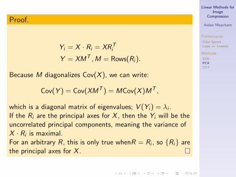
Proof.

Yi = X · Ri = XRTi

Y = XMT ,M = Rows(Ri ).

Because M diagonalizes Cov(X ), we can write:

Cov(Y ) = Cov(XMT ) = MCov(X )MT ,

which is a diagonal matrix of eigenvalues; V (Yi ) = λi .If the Ri are the principal axes for X , then the Yi will be theuncorrelated principal components, meaning the variance ofX · Ri is maximal.For an arbitrary R, this is only true whenR = Ri , so {Ri} arethe principal axes for X .


Compression

Aidan Meacham

Preliminaries

Color Spaces

Lossy vs. Lossless

Methods

SVD

PCA

DCT

PCA Compression

I Given d vectors X , transform into k vectors Y , k < d

I Discard Yk+1 to Yd vectors with a minimal loss of data

I Blocks of 8× 8 pixels selected; turned into vectors oflength 82 = 64

I N vectors stacked as rows into a “class matrix” HN×64after subtracting the mean

I Calculate modal matrix, then project data using asmany principal components as we like


Compression

Aidan Meacham

Preliminaries

Color Spaces

Lossy vs. Lossless

Methods

SVD

PCA

DCT

PCA Remarks

I Less stable than SVD

I Better for extremely large data sets

I Big data - consumer modeling


Compression

Aidan Meacham

Preliminaries

Color Spaces

Lossy vs. Lossless

Methods

SVD

PCA

DCT

Discrete Cosine Transform

Definition

The one-dimensional DCT can be written as follows, whereφk is a vector with components n, written as a variable toavoid confusion with matrix notation

φk(n) =

√

2N cos

(2n+1)kπ2N , for n = 1, 2, . . . ,N − 1,√

1N , for n = 0.


Compression

Aidan Meacham

Preliminaries

Color Spaces

Lossy vs. Lossless

Methods

SVD

PCA

DCT

DCT Properties

I A set of k vectors (each of dimension n) is orthonormal

I The matrix of columns M = [φ0|φ1| . . . |φN−1] isinvertible by its transpose

I 2D case: apply transformation first to rows, then tocolumns (separable; composition of function along eachdimension)

I A matrix of values can be transformed via thecalculation B = MAMT


Compression

Aidan Meacham

Preliminaries

Color Spaces

Lossy vs. Lossless

Methods

SVD

PCA

DCT

JPEG File Format

I JPEG utilizes DCT

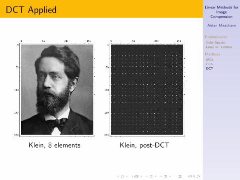
I Applying DCT moves information to lower indices(vector or matrix)

I Higher index entries close to zero

I Lossy compression - quantization

I Settings - force the last n indices of a vector to zero

I For every 8× 8 submatrix, (8− n)2 coefficients out of64 nonzero


Compression

Aidan Meacham

Preliminaries

Color Spaces

Lossy vs. Lossless

Methods

SVD

PCA

DCT

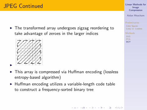
JPEG Continued

I The transformed array undergoes zigzag reordering totake advantage of zeroes in the larger indices

I

I This array is compressed via Huffman encoding (losslessentropy-based algorithm)

I Huffman encoding utilizes a variable-length code tableto construct a frequency-sorted binary tree


Compression

Aidan Meacham

Preliminaries

Color Spaces

Lossy vs. Lossless

Methods

SVD

PCA

DCT

JPEG Remarks

I Only non-reversible step is quantization

I Reversing other steps (switching order of multiplication)retrieves image

I Data lost no matter what - rounding errors

I DCT transforms frequencies, not intensities - humaneye sensitivity / recognition

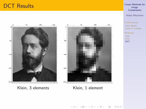
I Blocky artifacts - natural vs. manufactured images


Compression

Aidan Meacham

Preliminaries

Color Spaces

Lossy vs. Lossless

Methods

SVD

PCA

DCT

DCT ExampleSage

I Import image and convert to Sage matrix

I Create DCT matrix

I Subdivide matrix and apply transform

I Quantize

I Reconstitute


Compression

Aidan Meacham

Preliminaries

Color Spaces

Lossy vs. Lossless

Methods

SVD

PCA

DCT

DCT Applied

Klein, 8 elements Klein, post-DCT


Compression

Aidan Meacham

Preliminaries

Color Spaces

Lossy vs. Lossless

Methods

SVD

PCA

DCT

DCT Results

Klein, 8 elements Klein, 5 elements


Compression

Aidan Meacham

Preliminaries

Color Spaces

Lossy vs. Lossless

Methods

SVD

PCA

DCT

DCT Results

Klein, 3 elements Klein, 1 element


Compression

Aidan Meacham

Preliminaries

Color Spaces

Lossy vs. Lossless

Methods

SVD

PCA

DCT

References

I [1] Hoggar, S. G. Mathematics of digital images:creation, compression, restoration, recognition.Cambridge: Cambridge University Press, 2006.

I [2] N. Ahmed, T. Natarajan and K.R. Rao. “DiscreteCosine Transform.” IEEE Trans. Computers, 90-93,Jan. 1974.

I [3] Lay, David. Linear Algebra and its Applications.New York: Addison-Wesley, 2000.

I [4] Trefethen, Lloyd N., and David Bau. Numericallinear algebra. Philadelphia: Society for Industrial andApplied Mathematics, 1999.

linear methods for image compression - math 420, prof....

Documents