igcc power plant dispatch using infinite-horizon...

IGCC Power Plant Dispatch Using Infinite-Horizon Economic

Model Predictive Control

Journal: Industrial & Engineering Chemistry Research

Manuscript ID: ie-2012-008665.R2

Manuscript Type: Article

Date Submitted by the Author: n/a

Complete List of Authors: Omell, Benjamin; Illinois Insitute of Technology, Department of Chemical and Biological Engineering Chmielewski, Donald; Illinois Institute of Technology, Department of Chemical and Biological Engineering

ACS Paragon Plus Environment

Industrial & Engineering Chemistry Research

1

IGCC Power Plant Dispatch

Using Infinite-Horizon Economic Model Predictive Control

Benjamin P. Omell and Donald J. Chmielewski

1

Department of Chemical and Biological Engineering, Illinois Institute of Technology, Chicago, IL 60616

The Integrated Gasification Combined Cycle (IGCC) possesses a number of

benefits over traditional power generation plants, ranging from increased efficiency

to flex-fuel and carbon capture opportunities. A lesser known benefit of the IGCC

configuration is the ability to load track electricity market demands. The idea being

that process modifications to enable dispatch capabilities will allow for a time-shift

of power production away from periods of low energy value to periods of high value.

The work begins with an illustration of Economic Model Predictive Control (EMPC)

as a vehicle to exploit dispatch capabilities by pursuing directly the objective of

maximizing revenue. However, implementation of EMPC can result in unexpected

and at times pathological closed-loop behavior, including inventory creep and bang-

bang actuation. To address these issues, an infinite-horizon version of EMPC is

developed and shown avoid many of the performance issues observed in the finite-

horizon version. The paper concludes with an in depth discussion of energy value

forecasting and how the quality of forecasts can be incorporated into the design of the

infinite-horizon EMPC controller.

I. INTRODUCTION

Power plants based on the Integrated Gasification Combined Cycle (IGCC) possess a number

of benefits over traditional power generation, including increased efficiency and flex-fuel and

carbon capture opportunities. In short, a conventional IGCC power plant operates as in Figure 1,

but without the storage units or MeOH plant. The gasification block converts coal and oxygen

into synthesis gas, which is subsequently cleaned and de-carbonized to output a stream of nearly

pure hydrogen. This hydrogen is then converted to electric power by a combined cycle power

block. A portion of generated power must be used to drive compressors for air separation and

CO2 sequestration operations.

1 Corresponding author: phone: 312-567-3537; fax: 312-567-8874; e-mail: [email protected]

Page 1 of 40



123456789101112131415161718192021222324252627282930313233343536373839404142434445464748495051525354555657585960

2

Another possible benefit of IGCC is smart grid coordination through power output dispatch.

Specifically, it is postulated that an IGCC plant can change power output to track grid demand

and thus exploit electricity market price fluctuations. The ability to change power output from an

IGCC plant can be achieved by a variety of hardware configurations (see Figure 1). The

configuration most commonly cited is poly-generation. In this case, a portion of the hydrogen

from the acid gas removal unit is diverted elsewhere during periods of low energy value. This

diverted hydrogen could be sold directly or chemically converted to a liquid fuel (possibly

MeOH) for transportation applications, [Robinson and Luyben, 2011]. Another possibility is to

store the hydrogen during periods of low energy value, and then draw from the inventory during

peak demand periods. A similar scenario with respect to the Air Separation Unit (ASU) is also

possible. In this case, a compressed air storage unit is placed between the air compressor and the

cryogenic distillation units. Such a configuration would allow for a constant flow of compressed

air to the cryogenic distillation, while allowing the power to the air compressors to be anti-

correlated with energy value, which would add power to net output during periods of high value.

Similarly, significant power is consumed to compress CO2 to sequestration pressure. Thus, part

of the captured CO2 can be stored at an intermediate pressure during periods of high energy

value and eventually pressurized during low value periods. It is also noted that an unmodified

plant has dispatch capabilities, in the sense that the gasification block can be asked to change

hydrogen production rates. However, the ramp rate of the gasification block is expected to be

quite slow, owing mostly the slow response time of the cryogenic distillation portion of the ASU,

[Jones et al., 2011].

A fundamental question associated with smart grid coordination is the development of a

control structure capable of accepting information from the smart grid. The first issue concerns

set-point tracking abilities. Specifically, one must design regulatory level loops to achieve

desired set-point ranges and ramp rate capabilities. A number of efforts have explored this issue

for a variety of IGCC configurations as well as specific unit operations [Mahapatra and Bequette,

2010; Bequette and Mahapatra, 2010; Jones et al., 2011; Robinson and Luyben, 2011]. While

controller design at the regulatory level is clearly an important activity, such efforts typically

lack sufficient motivation. That is, the performance objectives of desired set-point ranges and

achievable ramp rates are set somewhat arbitrarily. To arrive at sufficient motivation for these

objectives, one must consider the supervisory controller, which will ask the regulatory

Page 2 of 40



123456789101112131415161718192021222324252627282930313233343536373839404142434445464748495051525354555657585960

3

controllers to implement its set-point commands. Two scenarios are possible. The first is a

situation in which the regulatory loops are overdesigned. That is, the controllers are capable of

achieving performance greater than the supervisory controller would ever request. In this case,

there is likely over-expenditure regarding control system hardware. The second scenario is a

situation in which the regulatory loops are incapable of achieving the performance desired by the

supervisor. In this case, the regulatory loops could be redesigned (by adding more effective

hardware) or the performance limitations of the regulatory loops could be communicated to the

supervisor, so that it knows the level of performance that is possible and can plan accordingly.

One way to define a supervisory controller is to assume a merchant style of operation.

Specifically, set the goal to be maximization of average revenue, defined as the integral of the

product of energy value and net power produced. In this case, the energy value signal would be

an input to the controller. However, unlike a disturbance, the objective is not to kill its impact on

the output. Similarly, unlike a set-point command, the objective is not to force the output to track

energy value (however, as we will see in subsequent sections, the set-point analogy is very close

to the resulting objective). One way to approach this problem is through the use of Economic

Model Predictive Control (EMPC), [Rawlings and Amrit, 2009]. In this case, the quadratic

objective function typically used in MPC, [Rawlings, 2000], is replaced by an expression directly

reflecting revenue. Similar approaches have worked well in the area of Heating Ventilation and

Air Conditioning (HVAC) control, [Braun, 1992; Morris et al., 1994; Kintner-Meyer and Emery,

1995; Henze et al., 2003; Braun, 2007; Mendoza-Serrano and Chmielewski, 2012a], as well as in

the area of process operations scheduling [Karwana and Keblisb, 2007; Baumrucker and Biegler,

2010; Lima et al., 2011, Kostina et al., 2011]. In both of these applications computational issues,

resulting from the large size of the on-line optimization problem, have been reported. Efforts to

reduce this computational burden, by reducing prediction horizon, have resulted in undesirable

closed-loop characteristics, including inventory creep, [Lima et al., 2011] and bang-bang type

actuation [Mendoza-Serrano and Chmielewski, 2012a]. It is also noted that efforts to ensure

closed-loop stability of the EMPC algorithm have required the use of specialized analysis

techniques and non-intuitive additions to the basic algorithm [Diehl, et al., 2011; Huang and

Biegler, 2011; Heidarinejad, et al., 2012].

The next section outlines the EMPC approach and illustrates, through a simplified IGCC

example, its ability to maximize revenue. In addition, the closed-loop eccentricities of the EMPC

Page 3 of 40



123456789101112131415161718192021222324252627282930313233343536373839404142434445464748495051525354555657585960

4

are illustrated. Section 3 introduces a new class of linear controllers. This new class, denoted

Economic Linear Optimal Control (ELOC), is shown to possess a policy similar to EMPC, but

only capable of enforcing equipment constraints from a statistical perspective. In Section 4, the

infinite-horizon EMPC controller is developed using ELOC as a basis. Section 5 discusses the

important issue of forecasting energy value and the development of a measurement based

formulation of the infinite-horizon EMPC policy.

II. ECONOMIC MPC

Consider a process model: ),,( pmsfs =& , ),,( pmshq = where s is the state vector, m is the

vector of manipulated variables, p is the disturbance vector and q contains the performance

outputs. In addition, assume the following restrictions on the performance outputs:

maxmin qqq ≤≤ . To implement a predictive type controller, first the continuous-time model must

be converted to discrete-time form and second, the notion of a predictive time index must be

introduced. The resulting model is:

))|(ˆ),|(),|(()|1( ikpikmiksfiks d=+

(1)

))|(ˆ),|(),|(()|( ikpikmikshikq d=

(2)

maxmin )|( qikqq ≤≤

(3)

)(ˆ)|( isiis =

(4)

where the index i represents the actual time of the process and the index k is predictive time. The

idea being that at a time i the controller will be given an estimate of the initial condition, )(ˆ is ,

along with forecasts of the process disturbances, )|(ˆ ikp . Then, the controller must select a

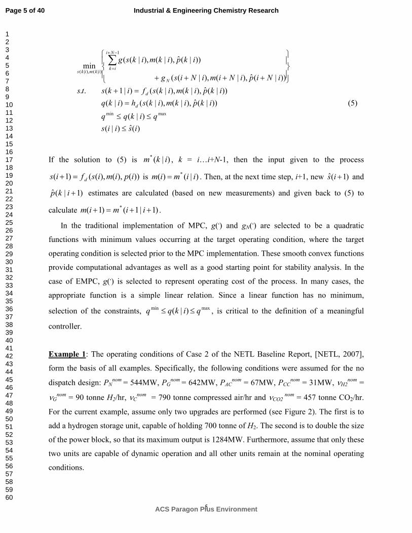
sequence of control inputs )|( ikm , k = i…i+N-1, such that the inequalities of (3) are satisfied.

As there may be many sequences satisfying (3), an additional performance measure is applied

via the following optimization problem:

Page 4 of 40



123456789101112131415161718192021222324252627282930313233343536373839404142434445464748495051525354555657585960

5

)(ˆ)|(

)|(

))|(ˆ),|(),|(()|(

))|(ˆ),|(),|(()|1(..

))|(ˆ),|(),|((

))|(ˆ),|(),|((min

maxmin

1

)|(),|(

isiis

qikqq

ikpikmikshikq

ikpikmiksfiksts

iNipiNimiNisg

ikpikmiksg

d

d

N

Ni

ikikmiks

≤

≤≤

=

=+

++++

∑−+

=

(5)

If the solution to (5) is )|(* ikm , k = i…i+N-1, then the input given to the process

))(),(),(()1( ipimisfis d=+ is )|()( * iimim = . Then, at the next time step, i+1, new )1(ˆ +is and

)1|(ˆ +ikp estimates are calculated (based on new measurements) and given back to (5) to

calculate )1|1()1( * ++=+ iimim .

In the traditional implementation of MPC, g(.) and gN(.) are selected to be a quadratic

functions with minimum values occurring at the target operating condition, where the target

operating condition is selected prior to the MPC implementation. These smooth convex functions

provide computational advantages as well as a good starting point for stability analysis. In the

case of EMPC, g(.) is selected to represent operating cost of the process. In many cases, the

appropriate function is a simple linear relation. Since a linear function has no minimum,

selection of the constraints, maxmin )|( qikqq ≤≤ , is critical to the definition of a meaningful

controller.

Example 1: The operating conditions of Case 2 of the NETL Baseline Report, [NETL, 2007],

form the basis of all examples. Specifically, the following conditions were assumed for the no

dispatch design: PNnom = 544MW, PG

nom = 642MW, PACnom = 67MW, PCC

nom = 31MW, νH2nom =

νGnom = 90 tonne H2/hr, νC

nom = 790 tonne compressed air/hr and νCO2 nom = 457 tonne CO2/hr.

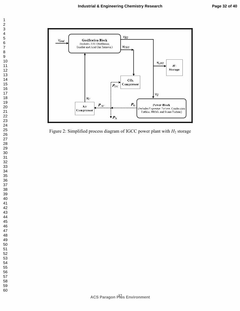
For the current example, assume only two upgrades are performed (see Figure 2). The first is to

add a hydrogen storage unit, capable of holding 700 tonne of H2. The second is to double the size

of the power block, so that its maximum output is 1284MW. Furthermore, assume that only these

two units are capable of dynamic operation and all other units remain at the nominal operating

conditions.

Page 5 of 40



123456789101112131415161718192021222324252627282930313233343536373839404142434445464748495051525354555657585960

6

Remark: It should be pointed out that the equipment upgrades of this example are selected

arbitrarily and intended only to illustrate the EMPC procedure. However, it is expected that

changes to the assumed equipment upgrade sizes will impact the revenue increase expected from

EMPC operation. Specifically, larger upgrades are expected to yield larger revenue increases. It

is additionally recognized that a proper economic assessment of the IGCC dispatch opportunity

will require a net present value calculation that weighs revenue gain against the capital cost of

equipment upgrades. While the preliminary results of [Yang et al., 2012] propose such a

procedure, many of the engineering challenges (associated with H2 storage facilities and

equipment degradation resulting from cycling of the power block) have yet to be addressed. In

sum, the current effort has the limited scope of assessing revenue gains under the assumption of

pre-specified and technologically viable equipment upgrades. As a final point, the assumption of

lower bounds at zero for both storage capacity and power block throughput is simply to enhance

presentation clarity. Specification of non-zero lower bounds is not expected to change the

qualitative aspects of subsequent results.

The top plot of Figure 3 indicates the energy values used for this example (this historic data

corresponds to the PJM Western Hub, Day-Ahead prices for the period of June 1, 2001 through

June 10, 2001, [PJM, 2012]). In the envisioned EMPC implementation, forecasts of energy value

will be provided to the controller. In addition to forecast errors, these forecasts are likely to be

updated at each time step. However, to avoid the details of forecasting and the closed-loop

impacts of forecast error and updates, this example will assume the forecasts to be perfect, in that

they are error free and do not change with time. While this assumption is not critical (and will be

removed in Section 4), it allows us focus on the fundamental issues and not wonder if observed

behavior is due to a forecasting artifact. (As such, in this example, the ‘hat’ notation will be

dropped.)

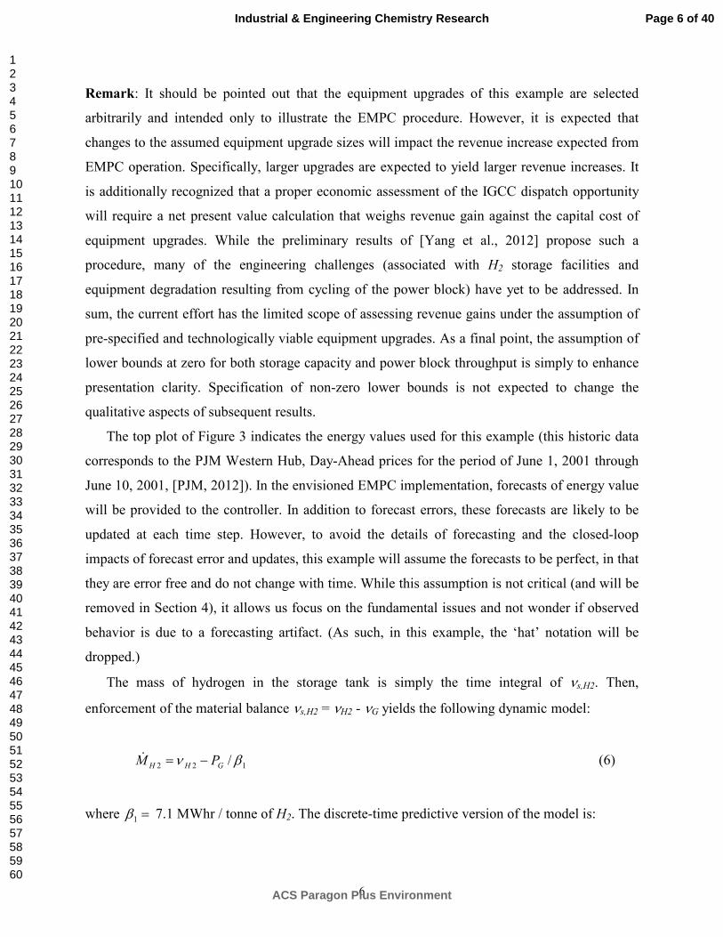
The mass of hydrogen in the storage tank is simply the time integral of νs,H2. Then,

enforcement of the material balance νs,H2 = νH2 - νG yields the following dynamic model:

122 / βν GHH PM −=& (6)

where =1β 7.1 MWhr / tonne of H2. The discrete-time predictive version of the model is:

Page 6 of 40



123456789101112131415161718192021222324252627282930313233343536373839404142434445464748495051525354555657585960

7

1...

)|(0

)|(0

)|()|()|1(

max

max

22

22

−+=

≤≤

≤≤

+−=+

Niik

PikP

MikM

cikbPikMikM

GG

HH

GHH

(7)

If the sample time is ∆ts = 1 hr then b = ∆ts/β1 = 0.141 tonne H2/MW and c = ∆tsνH2 = 90 tonne

H2, MH2max = 700 tonne H2 and PG

max = 1284 MW. It is noted that selecting a value of zero for

PG will result in negative values for PN. However, this should not be an issue, as this power

should be available from the grid, and most likely at a low price.

If )(iCe denotes energy value during period i, then revenue during period i is sNe tiPiC ∆)()(

sCCACesGe tPPiCtiPiC ∆+−∆= ))(()()( . Since the second term cannot be influenced by the

manipulated variable, )(iPG , an appropriate formulation of the EMPC on-line optimization is

)()|(

1...

)|(0

)|(0

)|()|()|1(..

)|()|(max

22

max

max

22

22

1

)|(),|(2

iMiiM

Niik

PikP

MikM

cikbPikMikMts

ikPikCN

t

HH

GG

HH

GHH

Ni

ik

Ges

ikPikM GH

=

−+=

≤≤

≤≤

+−=+

∆

∑−+

=

(8)

where the constant Nts /∆ may be dropped, but is retained so that the units of the objective

function will be equal to those of average revenue. Clearly, problem (8) can be solved using a

standard LP solver.

Figure 3 illustrates the closed-loop response of the EMPC policy using a 24 hour prediction

horizon (N = 24). In this case, the response of the manipulated variable, PG, is as one would

desire; at its maximum when energy value is high and at its minimum when energy value is low.

The periods in which PG is at the nominal value (PGnom = 642MW = β1νH2) correspond to

intervals in which the hydrogen storage is full and energy value is low or the storage is empty

and energy value is high. This behavior, however, makes good sense as the controller has no

Page 7 of 40



123456789101112131415161718192021222324252627282930313233343536373839404142434445464748495051525354555657585960

8

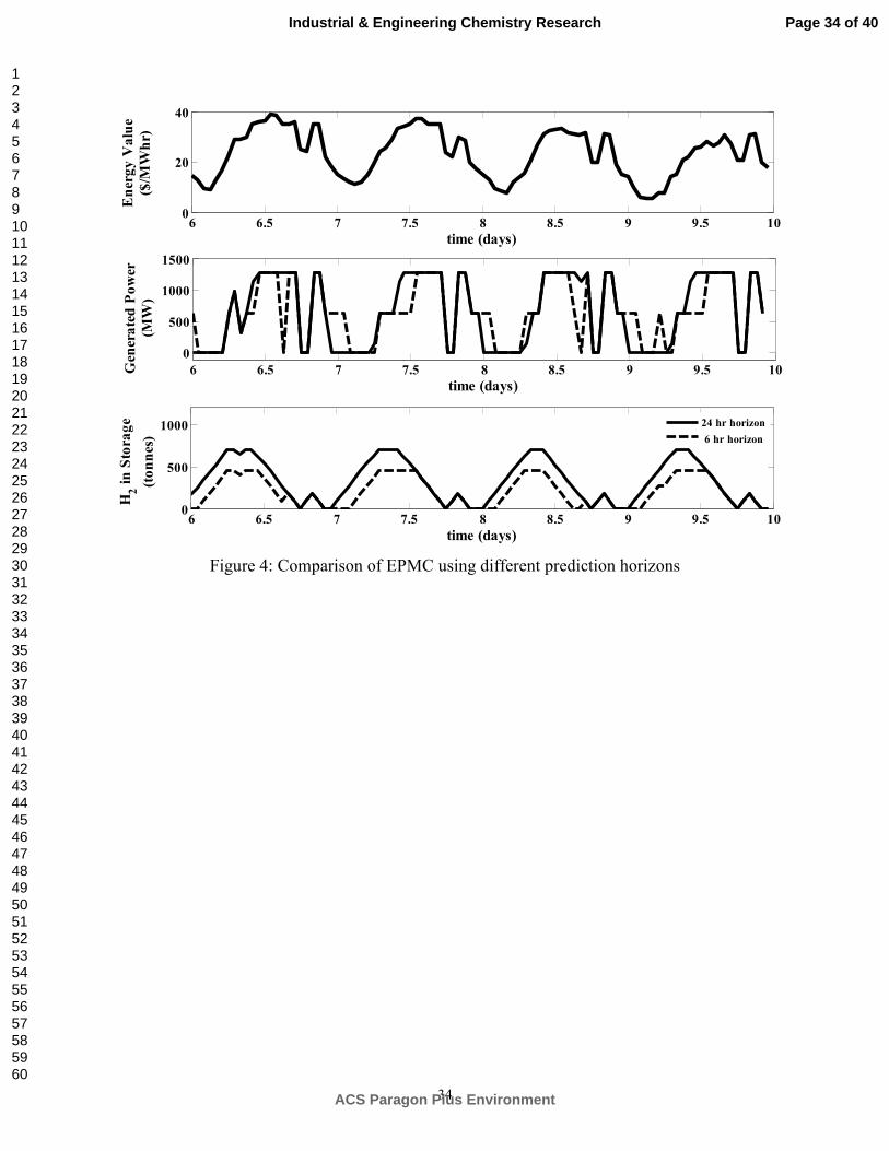
other reasonable option under these conditions. In the 6 hour horizon case (of Figure 4), the

EMPC policy seems to lose this good sense. That is, the controller tends to set PG equal to the

nominal value more frequently than needed. Specifically, during periods in which energy value

is low and the storage is not yet full. Why would the controller perform this way? The answer

obviously stems from the abbreviated horizon. As stated in [Lima et al., 2011], the controller is

‘myopic’, in the sense that it cannot see beyond its short horizon. And as such, the controller

decides to use up the hydrogen it has in inventory in an effort to maximize short-term revenue.

However, as illustrated by the 24 hour horizon case, if it had known that the value of converting

hydrogen to electric energy would soon increase, then it would have continued to stockpile

hydrogen rather than use it. One approach to mitigating the inventory creep phenomena is to add

a constraint to the final step of the horizon. Specifically, require the predicted inventory at the

final step to be greater than some fixed value, [Lima et al., 2011]. While this method can reduce

the impact of inventory creep, it will also require an ad’hoc selection of the lower bound

parameters.

It is also noted that in both the 24 and 6 hour horizon cases, there are intervals in which PG

jumps from one extreme to the other and then back to the original extreme. This sort of

chattering (or bang-bang type actuation) seems to occur when the inventory is at an extreme and

the energy value is near its average or when the energy value curve experiences sharp changes

(for example at the second, small, daily peak occurring in the early evening). To reduce the

occurrence of this chatter one could add constraints to the first or second time derivative of PG.

In [Baumrucker and Biegler, 2010], the square of the first derivative of the manipulated variable

is added to the objective function. However, both of these derivative based methods seem to be

poorly motivated by the physical situation and will likely compromise optimality of the closed-

loop response. Another approach is to force power output to be in one of three states; 0, PGnom or

PGmax. Then, one could add constraints prohibiting two state changes within a certain period (say

3 or 4 hours). In addition to requiring the use of mixed-integer programming to solve the on-line

EMPC optimization problem, selection of an appropriate waiting period is somewhat arbitrary.

Another approach, and the one advocated in this paper, is to extend the horizon size of the

EMPC to infinity. Extending the constrained EMPC problem to an infinite horizon problem

would, however, result in an infinite number of variables in the numeric optimization and render

the problem intractable. A common approach to similar constrained infinite-time optimal control

Page 8 of 40



123456789101112131415161718192021222324252627282930313233343536373839404142434445464748495051525354555657585960

9

problems is to enforce only a finite number of constraints, [Chmielewski and Manousiouthakis,

1996; Manousiouthakis and Chmielewski, 2002]. In this case, the unconstrained infinite-horizon

tail is solved analytically and its value function is appended to the constrained finite-time

problem as a final cost term, representing the cost-to-go from the final time to infinity. However,

if the EMPC objective function for the IGCC problem is applied to an unconstrained problem,

the problem will become unbounded and no solution will exist. Thus, our approach will be to

modify the unconstrained infinite-horizon tail problem to be statistically constrained in an effort

to obtain an analytical solution and approximate the cost-to-go from the final time to infinity.

III. ECONOMIC LINEAR OPTIMAL CONTROL

We now explore the question of developing a linear controller capable of mimicking the EMPC

policy. To motivate the discussion, the scenario of Example 1 will be assumed. However,

generalization of the approach is straightforward; see [Yang et al., 2012]. The resulting

Economic Linear Optimal Control (ELOC) policy will form the basis of the infinite-horizon

EMPC policy to be developed in Section 4.

We begin by revisiting the EMPC objective function and consider the impact of taking the

limit with respect to N.

[ ] sGe

Ni

ik

Ges

NtPCEikPikC

N

t∆=

∆

∑−+

=∞→

1

)|()|(lim (9)

The result is that the objective function will become the long term average revenue. The question

then becomes, can one calculate this long term average and can one select a policy for PG such

that this average is maximized? One approach is to assume PG has the following form:

=GP~

eC~

α (10)

where GGG PPP −=~

, eee CCC −=~

, GP = E[ GP ] and eC = E[ eC ]. Equation (10) reflects the

general notion that when energy value is high, power production should be large and production

should be small when value is low. The parameter α, yet to be specified, will indicate the

Page 9 of 40



123456789101112131415161718192021222324252627282930313233343536373839404142434445464748495051525354555657585960

10

magnitude of this relationship. The consequence of (10) is that (9) can be evaluated as:

GeCeGeGeGGeeGe PCPCPCEPPCCEPCE +Σ=+=++= α]~~

[)]~

)(~

[(][ (11)

where ]~

[2

eCe CE=Σ is the variance of the energy value signal. Thus, if given a characterization

of Ce, then one could simply optimize over α and GP . (However, for the case being considered,

inspection of (6) indicates that GP must be equal to νH2/β1 regardless of the control policy

selected.)

A stochastic characterization of Ce begins by recalling the historic energy value data depicted

in Figure 3. The data clearly possesses an oscillatory characteristic with a period of 1 day. As

such, one could model Ce as the output of an under-damped 2nd order system driven by white

noise (think of a mass-spring-damper system with a harmonic frequency of 1 day-1). However,

experience indicates that such a model will allow too much of the low frequency energy

contained in the white noise to be passed through to Ce. To remove these low frequency

components, the white noise is first sent through a high pass filter. The net result is the following

3rd order shaping filter:

ee

h

ccc

CC

w

w

+=

−=

−−−=

=

αφ

τφαφ

φχωφωφαωφ

φφ

/

/)(

2)(

1

313

21

2

31

2

2

21

&

&

&

(12)

where cc τπω /2= , 24=cτ hr, 1.0=χ , 1=hτ hr and w1 is a Gaussian, zero-mean white noise

process with the following spectral density:

eC

hc

hchc

c

wS Σ

++

=

22

22 1241 τω

τχωτωω

χ (13)

The idea behind this shaping filter model is that for all parameter values ( cτ , χ , hτ , eC and α ),

Page 10 of 40



123456789101112131415161718192021222324252627282930313233343536373839404142434445464748495051525354555657585960

11

a stochastic covariance analysis on (12) will indicate that the calculated variance of eC is equal to

the CeΣ parameter value selected in (13). As such, it is highlighted that the cτ , χ , hτ values

selected above are not special, but simply represent parameter values such that realizations of Ce

match, purely on a visual basis, with the data of Figure 3. While this is sufficient for our purpose

of illustrating the method, a more rigorous system identification approach is likely warranted,

which may include changing the model structure from that given in (12). The top plot of Figure 5

is a realization of eC generated from (12) using the above parameters as well as; α = 1 MW2hr/$,

eC = 20 $/MWhr and CeΣ = (12 $/MWhr)2.

An important aspect of the definition of Ce is the fact that φ1 is equal to eC~

α . Thus, to

enforce an approximation of condition (10), one could require

( )[ ] εφ <−2

1

~GPE (14)

where ε is selected to be sufficiently small, but not so small that numeric feasibility becomes an

issue. However, since PG is the manipulated variable, satisfaction of this inequality should be

achievable for rather small values of ε (ε is set to 0.01 MW2 for all cases).

The next step is to recast the compound system into deviation variable form:

T

HH MMx ][ 32122 φφφ−=

][ GG PPu −= ][ 1ww = (15)

T

GGGGHH PPPPMMz ])([ 122 φ−−−−=

where 2HM is arbitrarily defined as 2/max

2HM . Then, the process (augmented with the shaping

filter) can be written as

maxmin zzz

uDxDz

GwBuAxx

ux

≤≤

+=

++= α&

(16)

Page 11 of 40



123456789101112131415161718192021222324252627282930313233343536373839404142434445464748495051525354555657585960

12

where

−

−−−=

h

ccc

A

τωχωω/1000

20

0100

0000

22

−

=

0

0

0

/1 1β

B

=

h

c

G

τω/1

0

0

2 [ ]1ww SS = (17)

−

=

0010

0000

0001

xD

=

1

1

0

uD

−

−

−

=

εG

H

P

M

z

2

min

−

−

=

εGG

HH

PP

MM

z max

2

max

2

max

(18)

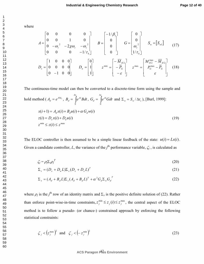
The continuous-time model can then be converted to a discrete-time form using the sample and

hold method ( stA

d eA∆= , ∫

∆

=st

At

d BdteB0

, ∫∆

=st

At

d GdteG0

and sww tS ∆=Σ / ), [Burl, 1999]:

maxmin )(

)()()(

)()()()1(

zizz

iuDixDiz

iwGiuBixAix

ux

ddd

≤≤

+=

++=+ α

(19)

The ELOC controller is then assumed to be a simple linear feedback of the state: )()( iLxiu = .

Given a candidate controller, L, the variance of the jth performance variable, ζj , is calculated as

ζj = ρjΣzρjT (20)

T

xxxuxz LDDLDD )()( +Σ+=Σ (21)

T

dwd

T

ddxddx GGLBALBA Σ++Σ+=Σ 2)()( α (22)

where ρj is the jth row of an identity matrix and Σx is the positive definite solution of (22). Rather

than enforce point-wise-in-time constraints,maxmin )( jjj zizz ≤≤ , the central aspect of the ELOC

method is to follow a pseudo- (or chance-) constrained approach by enforcing the following

statistical constraints:

( )2max

jj z<ζ and ( )2min

jj z−<ζ (23)

Page 12 of 40



123456789101112131415161718192021222324252627282930313233343536373839404142434445464748495051525354555657585960

13

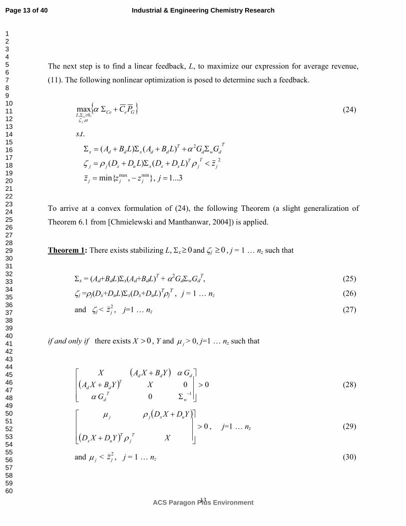
The next step is to find a linear feedback, L, to maximize our expression for average revenue,

(11). The following nonlinear optimization is posed to determine such a feedback.

{ }GeCeL

PC

j

x

+Σ≥Σ

ααζ ,

,0,max (24)

3...1},,min{

)()(

)()(

..

minmax

2

2

=−=

<+Σ+=

Σ++Σ+=Σ

jzzz

zLDDLDD

GGLBALBA

ts

jjj

j

T

j

T

xxxuxjj

T

dwd

T

ddxddx

ρρζ

α

To arrive at a convex formulation of (24), the following Theorem (a slight generalization of

Theorem 6.1 from [Chmielewski and Manthanwar, 2004]) is applied.

Theorem 1: There exists stabilizing L, Σx 0≥ and ζj 0≥ , j = 1 … nz such that

Σx = (Ad+BdL)Σx(Ad+BdL)T + α2GdΣwGd

T, (25)

ζj =ρj(Dx+DuL)Σx(Dx+DuL)TρjT , j = 1 … nz (26)

and ζj < 2

jz , j=1 … nz (27)

if and only if there exists X 0> , Y and jµ > 0, j=1 … nz such that

( )( ) 0

0

01

>

Σ

+

+

−w

T

d

T

dd

ddd

G

XYBXA

GYBXAX

α

α (28)

( )

( )0>

+

+

XYDXD

YDXD

T

j

T

ux

uxjj

ρ

ρµ

, j=1 … nz (29)

and jµ < 2

jz , j = 1 … nz (30)

Page 13 of 40



123456789101112131415161718192021222324252627282930313233343536373839404142434445464748495051525354555657585960

14

Application of Theorem 1 to (24), results in the following convex optimization.

{ }GeCeXY

PC

j

+Σ≥

ααµ ,

,0,max (31)

( )( )

( )

( )

3...1},,min{

0

0

0

0

..

minmax

2

1

=−=

<

>

+

+

>

Σ

+

+

−

jzzz

z

XYDXD

YDXD

G

XYBXA

GYBXAX

ts

jjj

jj

T

j

T

ux

uxjj

w

T

d

T

dd

ddd

µ

ρ

ρµ

α

α

Due to the linearity of the objective function and convexity of the constraints any local optimum

of problem (31) is guaranteed to be a global optimum. It is additionally noted that if the solution

to (31) is X* and Y*, then L* = Y*(X*)-1 is the solution to (24), within the accuracy of the strict

inequality constraints of (31). To arrive at the ELOC policy, the solution L* must be scaled with

respect to α*. That is, the columns of L* corresponding to the shaping filter states (the 2nd through

4th states) must be multiplied by α*. This rescaling will make the policy appropriate for a price of

electricity generated by (12) with α set equal to 1.

Example 2a: Reconsider the scenario of Example 1, and assume the shaping filter used to model

Ce has parameter values as indicated in this section. Problem (31) is solved using the Linear

Matrix Inequality (LMI) optimization routines found in the Robust Control Toolbox of Matlab.

The solution to problem (31) is found to be α* = 774 MW2hr/$ and

[ ]0009.0017.0018.0067.0* −−=L (32)

After rescaling with respect to α*, the ELOC feedback gain is determined to be:

Page 14 of 40



123456789101112131415161718192021222324252627282930313233343536373839404142434445464748495051525354555657585960

15

[ ]69.09.122.14067.0 −−=ELOCL (33)

The second two plots of Figure 5 compare the resulting ELOC policy with the EMPC policy

using the energy value data of the first plot of Figure 5. As expected the ELOC policy does not

enforce constraints point-wise-in-time, but does enforce them statistically. The important point,

however, is that the ELOC trajectory has a general shape that is remarkably similar to the EMPC

trajectory.

It should be pointed out that a trajectory with less point-wise-in-time constraint violations

could be achieved by tightening the statistical constraints of the ELOC. (For example, in (31),

�� ̅� could be replaced with�� ̅ 2⁄ �

�.) This however would still not guarantee that

point-wise-in-time constraints would not be violated, only that they would be violated less

frequently. Furthermore, if the statistical constraints are tightened too much, then the trajectory

would be significantly altered from that of the EMPC. The next section will illustrate a novel

approach to enforce point-wise-in-time constraints while preserving the positive features of the

ELOC.

IV. INFINITE-HORIZON ECONOMIC MPC

We now turn to the question of converting the ELOC policy into one that is capable of enforcing

constraints point-wise-in-time. To do so, we revisit the quadratic version of MPC and highlight

the following important property. Consider an unconstrained finite-horizon MPC controller:

)()|(

1...),|()|()|1(..

))|()|()|(

)|(

)|(

)|(min

1

)|(),|(

ixiix

NiikikuBikxAikxts

iNiPxiNixiku

ikx

RM

MQ

iku

ikx

dd

TNi

ikT

T

ikuikx

≤

−+=+=+

+++

∑

−+

=

(34)

Then, the property is stated as follows: If P is selected such that

T

d

T

dd

T

dd

T

dd

T

d PBAMPBBRPBAMQPAAP )())(( 1 +++−+= − (35)

Page 15 of 40



123456789101112131415161718192021222324252627282930313233343536373839404142434445464748495051525354555657585960

16

then the MPC controller of (34) will be independent of horizon size, N, and will be identical to

using the following linear feedback gain

T

d

T

dd

T

d PBAMPBBRL )()( 1 ++−= − (36)

An equivalent statement would be: )()|(* iLxiiu = .

The first important point is the independence of the policy with respect to horizon size, which

is made possible by the appropriate selection of P. In essence, selecting P based on (35) makes

all unconstrained finite-horizon MPC policies equal to the infinite-horizon policy, which is the

classic linear quadratic regulator feedback given in (36).

The second important point is that for some linear feedbacks there exists an equivalent

unconstrained MPC controller. Thus, if such a property holds for the feedback generated by (31),

then the addition of constraints to its MPC counterpart will generate a policy similar to the

original linear feedback. In [Chmielewski and Manthanwar, 2004], it is shown that a class of

problems (to which (31) is a member) is guaranteed to possess an equivalent unconstrained MPC

controller. Furthermore, [Chmielewski and Manthanwar, 2004] provides the following Theorem

on inverse optimality, which can be used to synthesize weighting matrices Q, R, M and P (from

L, Ad and Bd) such that the resulting unconstrained MPC is equivalent to the original policy

)()( iLxiu = . Theorem 6.2 of [Chmielewski and Manthanwar, 2004] is restated here for

convenience.

Theorem 2: If there exists P > 0 and R > 0 such that

( ) ( )( ) 0>

++

++++−

RPABLPBBR

PBAPBBRLLPBBRLPAAP

d

T

dd

T

d

d

T

dd

T

d

T

d

T

d

T

d

T

d (37)

then ( )LPBBRLPAAPQ d

T

d

T

d

T

d ++−=̂ and ( ) d

T

dd

T

d

T PBAPBBRLM ++=̂ will be such that

Page 16 of 40



123456789101112131415161718192021222324252627282930313233343536373839404142434445464748495051525354555657585960

17

0>

RM

MQT

and P and L satisfy (35) and (36).

In summary, construction of the infinite-horizon EMPC is as follows. Begin by solving

problem (31) to determine ELOCL . Then, implement the procedure suggested by Theorem 2 to

synthesize weighting matrices Q, R, M and P that are companion to ELOCL . Finally, implement

the following constrained MPC policy using a standard QP solver.

)(ˆ)|(

1...,)|(

1...),|()|()|(

1...),|(ˆ)|()|()|1(..

))|()|()|(

)|(

)|(

)|(min

maxmin

1

)|(),|(

ixiix

Niikzikzz

NiikikuDikxDikz

NiikikwGikuBikxAikxts

iNiPxiNixiku

ikx

RM

MQ

iku

ikx

ux

ddd

TNi

ikT

T

ikuikx

≤

−+=≤≤

−+=+=

−+=++=+

+++

∑

−+

=

(38)

Example 2b: Continuing Example 2a, the linear feedback (33) generates the weighting matrices:

−−

−××−

×−×−

−−

=

16843130034200162

313001083.51037.63021

342001037.61096.63304

162302133047.15

55

55

Q [ ]3482=R (39)

−

−

=

2418

45000

49300

234

M 3

2

10

6660224192.0

22487605405.12

195404982.2

2.05.122.21026.7

−

−

×

−−

−

−

×

=P (40)

It is noted that the weighting matrices Q, R, M and P are not unique, in that identical

implementations of Theorem 2 on different computers or different versions of Matlab will likely

result in different weights. The important aspect, however, is to verify that a substitution of the

Page 17 of 40



123456789101112131415161718192021222324252627282930313233343536373839404142434445464748495051525354555657585960

18

weights back into (35) and (36) re-generates the policy ELOCL .

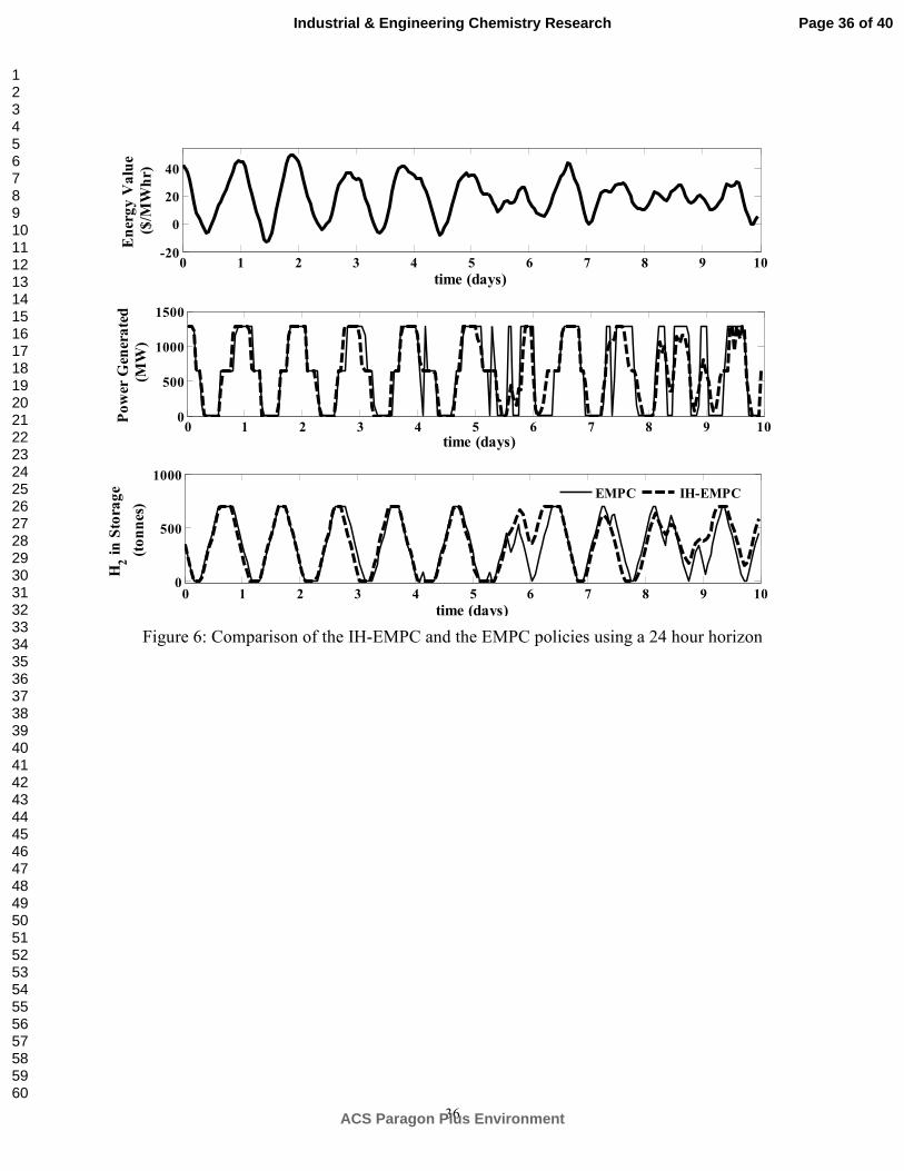
Using a 24 hour horizon and the energy values depicted in the top plot of Figure 6 (the same

as in Figure 5), the EMPC policy is compared to the infinite-horizon EMPC (IH-EMPC).

Clearly, there is a strong resemblance between the two policies. More remarkable is the fact that

the chatter observed in the EMPC seems be damped out almost completely. That is, the IH-

EMPC policy shows a tendency toward the chatter actions but is slowed by the move

suppression aspects of the quadratic objective. The plots of Figure 7 illustrate the policy’s

insensitivity with respect to horizon size. The fact that even with a horizon of one hour (one

time-step of prediction) the trajectory is virtually unchanged indicates the strong influence of the

final cost term: ))|()|( iNiPxiNix T ++ .

V. PARTIAL STATE INFORMATION IH-EMPC

While the plots of Figures 6 and 7 are impressive, the scenario of Example 2 provides the IH-

EMPC policy with two unrealistic advantages; perfect forecasting and the energy value data was

generated by the shaping filter model contained within the IH-EMPC policy. The assumption of

perfect forecast boils down to assuming perfect knowledge of the white noise sequence w(k) for

k > i, where i is the current time. In terms of problem (38), that is )()|(ˆ kwikw = for all i. In the

imperfect forecasting case, the procedure is as follows. Using a shaping filter model, such as the

one in Equation (12) with α =1, apply a state estimator to determine )(ˆ ix . Then, implement a

state predictor (essentially a simulation of (12) with )(ˆ)|( ixiix = and 0)|(ˆ =ikw ) to generate

forecasts )|( ikx . Application of this procedure to the historic data of Example 1 (top plot of

Figure 3) resulted in the plots of Figure 8. Clearly, both policies fail. The problem seems to be an

over-compensation for the short-term average of energy value. That is, the controllers hoard H2

in the first half of the simulation (t < 10 days), due to the fact that eC is less than eC (= 20

$/MWhr), and deplete H2 inventory in the second half, when eC is mostly greater than eC .

One way to address this issue is to restructure the shaping filter to capture the changes in the

short-term average. For example, the filter of (12) could be augmented with a low pass filter

driven by an independent white noise process. In this case (12) would be replaced with

Page 18 of 40



123456789101112131415161718192021222324252627282930313233343536373839404142434445464748495051525354555657585960

19

ee

l

h

ccc

CC

w

w

w

++=

−=

−=

−−−=

=

2411

4224

3113

21

2

311

2

2

21

//

/)(

/)(

2)(

αφαφ

τφαφ

τφαφ

φχωφωφαωφ

φφ

&

&

&

&

(41)

where 6=lτ hr and w2 is a Gaussian, zero-mean white noise process that is independent of w1

and the spectral densities of the two are defined as follows, with γ = 0.85:

eC

hc

hchc

c

wS Σ

++

=

22

22

1

124

τωτχωτω

ωχ

γ (42)

eClwS Σ−= τγ 2)1(2 (43)

One could then define z3 as 41

~φφ −−GP and let the optimization select α1 and α2 such that the

resulting policy will give appropriate weight to each state of the shaping filter (see [Mendoza-

Serrano and Chmielewski, 2012b] for details on the implementation of this procedure). The

result of the optimization is as one would expect, in that α2* is found to be zero, indicating that

the ELOC will place all its emphasis on short-term variability and ignore the short-term average.

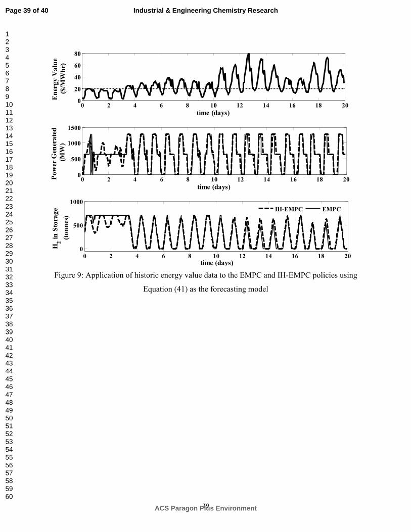
The result of using Equation (41) as the forecasting model is shown in Figure 9. In this case, both

policies perform much better. However, both still seem to have trouble when the short-term

average is significantly above or below eC . That is, in the first three days the policies hold on to

the H2 inventory for too long, and during the periods of 10-15 days and 17-20 days, the policies

do not store enough H2.

The problem stems from the fact that the policies think that the short-term variability can be

perfectly distinguished from the short-term average. However, in reality the state estimator

cannot perform this separation perfectly. Specifically, the estimator has available to it only the

energy value curve, which it models as the sum of φ1 and φ4. Then, it must separate the two

based only on frequency content. Thus, the problem with our previous IH-EMPC policy is that

the quality of the state estimator has not been communicated to the design procedure. To be able

Page 19 of 40



123456789101112131415161718192021222324252627282930313233343536373839404142434445464748495051525354555657585960

20

to communicate this estimator quality information, a Partial State Information (PSI) formulation

of the ELOC policy must be developed. We begin with a review of state estimation.

If given a process model )()()()1( iwGiuBixAix ddd ++=+ and a measurement equation

)()()( iFviCxiy += , where w and v are zero mean, Gaussian white noise sequences, then the

optimal (minimum error variance) state estimate, )(ˆ ix , is generated from the following system

[Anderson and Moore, 1979]:

( ))(ˆ)()()(ˆ)1(ˆ ixCiyKiuBixAix dd −++=+ (44)

where

( ) 1−Σ+ΣΣ= T

v

T

e

T

ed FFCCCAK (45)

and Σe is the positive definite solution to

( ) T

dwd

T

de

T

v

T

e

T

ed

T

dede GGACFFCCCAAA Σ+ΣΣ+ΣΣ−Σ=Σ−1

(46)

The following, easily verified, facts will be utilized in the subsequent development.

Fact 4.1: If the matrices Ad, C, Gd, Σw, F and Σv are block diagonal (with appropriate block

dimensions), then the matrices K and Σe will be block diagonal. Specifically, if Ad = diag{Adj},

C = diag{Cj}, Gd = diag{Gdj}, Σw = diag{Σwj}, F = diag{Fj}, and Σv = diag{Σvj}, then K =

diag{Kj} and Σe = diag{Σej} where

( ) 1−Σ+ΣΣ= T

jjvj

T

jjej

T

jjejdj FFCCCAK (47)

( ) T

jdjwjd

T

jdjej

T

jjvj

T

jjej

T

jjejd

T

djjejdjeGGACFFCCCAAA Σ+ΣΣ+ΣΣ−Σ=Σ

−1

(48)

Page 20 of 40



123456789101112131415161718192021222324252627282930313233343536373839404142434445464748495051525354555657585960

21

Fact 4.2: If the matrices Ad, C, Gd and F are defined as

=

=

=

=

02

01

02

01

0

0

0

0 and ,0

0,

0

0

F

FF

G

GG

C

CC

A

AA

d

d

d

d

d

d αα

αα

(49)

then

[ ]0201

0

2

2021

0210

2

1 and KKKee

eee αα

αααααα

=

ΣΣ

ΣΣ=Σ (50)

where 0K and 0e

Σ are from (47) and (48), with j = 0. Furthermore,

( )

( ) [ ]T

de

T

de

T

v

T

eT

ed

T

ed

T

de

T

v

T

e

T

ed

ACACFFCCCA

CA

ACFFCCCA

00020001

1

00000

0002

0001

1

ΣΣΣ+Σ

Σ

Σ=

ΣΣ+ΣΣ

−

−

αααα (51)

Covariance analysis under the PSI feedback structure, )(ˆ)( ixLiu = , utilizes two important

properties of optimal state estimation. First, the optimal estimate, )(ˆ ix , and the error signal,

)(ˆ)(ˆ)( ixixie −= , are orthogonal in that 0)]()(ˆ[ =ieixE . An immediate consequence of this fact

is that exx Σ−Σ=Σ ˆ . The second important property is that the innovations sequence, defined as

( ))(ˆ)(ˆ)( ixCiyKi −=η , is a zero mean, white noise process with covariance

( ) T

dev

T

e

T

ed ACFFCCCA ΣΣ+ΣΣ=Σ−1

η (52)

Thus, given the estimator system

)(ˆ)(ˆ)()(

)()(ˆ)()1(ˆ

ˆ ixDixLDixDiz

iixLBAix

xux

dd

++=

++=+ η (53)

Page 21 of 40



123456789101112131415161718192021222324252627282930313233343536373839404142434445464748495051525354555657585960

22

the variance of the jth element of z is calculated as

ζj = ρjΣzρjT (54)

T

xex

T

xuxxxuxz DDDLDDDLDD Σ+++Σ++=Σ )()( ˆˆˆ (55)

ηΣ++Σ+=Σ T

ddxddx LBALBA )()( ˆˆ (56)

Theorem 3: There exists stabilizing L, 0ˆ ≥Σx and ζj 0≥ , j = 1 … nz such that

( ) T

dev

T

e

T

ed

T

ddxddx ACCCCALBALBA ΣΣ+ΣΣ++Σ+=Σ−1

ˆˆ )()( (57)

T

j

T

xexj

T

j

T

xuxxxuxjj DDDLDDDLDD ρρρρζ Σ+++Σ++= )()( ˆˆˆ (58)

and ζj < 2

jz , j=1 … nz (59)

if and only if there exists X 0> , Y and jµ > 0, j=1 … nz such that

( )( )

( )0

0)(

0

)(

>

Σ+ΣΣ

+

Σ+

v

T

e

TT

ed

T

dd

T

eddd

CCCA

XYBXA

CAYBXAX

(60)

( )

( )0

)(

)(

ˆ

ˆ

>

++

++Σ−

XYDXDD

YDXDDDD

T

j

T

uxx

uxxj

T

j

T

xexjj

ρ

ρρρµ, j=1 … nz (61)

and jµ < 2

jz , j = 1 … nz (62)

proof: If the matrices Σ�, ��, Σ�, �� and ζi of Theorem 1 are redefined as Σ��, ��Σ��,

��Σ�� Σ��, ��, and �� Σ�� then Theorem 3 will result.

Example 3: This example will continue the scenarios of Examples 1 and 2, but update the

shaping filter model to (41) and extend the ELOC method to the PSI framework. Consider the

following block diagonal process model:

=

1

1

0

00

00

00

d

d

d

d

A

A

A

A

=

0

0

0d

d

B

B

=

12

11

0

0

0

0

d

d

d

d

G

G

G

G

αα

Σ

Σ=Σ

1

0

0

0

w

w

w (63)

Page 22 of 40



123456789101112131415161718192021222324252627282930313233343536373839404142434445464748495051525354555657585960

23

=

1

1

0

00

00

00

C

C

C

C

=

12

11

0

0

0

0

F

F

F

F

αα

Σ

Σ=Σ

1

0

0

0

v

v

v (64)

where the elements of the first block are Ad0 = 1, Bd0 = -∆ts /β1, Gd0 = ∆ts , C0 = F0 = 1,

svw t∆=Σ=Σ /)1.0( 2

00 and the element of the second block are stA

d eA∆= 1

1, ∫

∆

=st

tA

d dtGeG0

111 ,

sww tS ∆=Σ /1

and svv tS ∆=Σ /11where

−

−

−−−=

l

h

cccA

ττ

ωχωω

/1000

0/100

02

001022

1

=

l

h

cG

ττ

ω

/10

0/1

0

002

1

=

2

1

0

0

w

w

wS

SS (65)

1wS and 2wS are as in Equations (42) and (43), [ ]10011 =C , 11 =F and 2

1 )1.0(=vS . The

performance output is defined as [ ]210 xxxx DDDD = , [ ]TuD 110=

[ ]2ˆ1ˆ0ˆˆ xxxx DDDD = ,

where [ ]TxD 0010 = , 00ˆ21 === xxx DDD ,

−

=

0001

0000

0000

1x̂D and

−

=

1000

0000

0000

2x̂D (66)

Finally, the zmax and zmin vectors are as in Example 2.

The third row of the performance output indicates an enforcement of the following

constraint:

[ ] 22

41 )ˆˆ~( εφφ <−−GPE (67)

The first point about (67) is that the manipulated variable, PG, is being forced to track the

Page 23 of 40



123456789101112131415161718192021222324252627282930313233343536373839404142434445464748495051525354555657585960

24

estimates of the shaping filter states. This is appropriate since the controller does not have access

to the ‘true’ state values, which in reality do not even exist. The second point concerns the use of

α1 and α2 in (63) and (64), which will allow the optimization to select how much weight it will

give to the short term variability, 11 /ˆ αφ , and how much to give to the short term average, 24 /ˆ αφ .

An evaluation of the average revenue in the context of (67), yields the following expression

[ ] 2211

~~αα ddCPE eG += (68)

where T

x

T

xd 41ˆ111ˆ11 ρρρρ Σ+Σ= , T

x

T

xd 41ˆ441ˆ12 ρρρρ Σ+Σ= , 111ˆ exx Σ−Σ=Σ , 1eΣ is the positive

definite solution to (48), with j = 1, and 1xΣ satisfies T

dwd

T

dxdx GGAA 1111111 Σ+Σ=Σ . Finally, use of

Theorem 3, along with Facts 4.1 and 4.2, the PSI version of the ELOC design problem, in

convex form, is stated as

{ }2211

,,,0,

21

max ααααµ

dd

j

XY+

≥ (69)

( )( )

( )

( )

( )( )

3...1},,min{

0

0

0

0

0

0

)(

)(

0

0

0

..

minmax

2

1112

1111

000

1

1111

00000

ˆ

ˆ

01

1

=−=

<

Σ

Σ

Σ

=

Σ+Σ

Σ+Σ=

>

++

++Σ−

>

+

+

jzzz

z

CA

CA

CA

M

CC

CCM

XYDXDD

YDXDDDD

MM

XYBXA

MYBXAX

ts

jjj

jj

T

ed

T

ed

T

ed

v

T

e

v

T

e

T

j

T

uxx

uxxj

T

j

T

xexjj

T

T

dd

dd

µ

αα

ρ

ρρρµ

Page 24 of 40



123456789101112131415161718192021222324252627282930313233343536373839404142434445464748495051525354555657585960

25

The solution to problem (69) is found to be α1* = 87.3 MW2hr/$ and α2* = -47.0 MW2hr/$ and

[ ]45.13-00000.53857.861-86.580.0445=ELOCL (70)

The fact that α2* turns out to be negative indicates that the policy recognizes a correlation

between 1φ̂ and 4φ̂ , in the sense that when the short-term average of 1φ̂ is greater than zero, the

short-term average of 4φ̂ will also be positive. Thus, the selection of a negative α2*, which

manifests as a negative value for the 9th element of LELOC, and has the effect of canceling out the

short-term average of 1φ̂ .

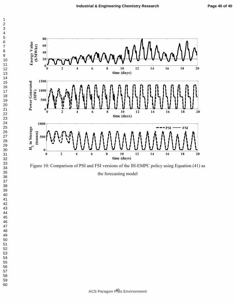
The plots of Figure 10 compare the PSI and FSI versions of the IH-EMPC policy. While

these trajectories appear to be very similar, the PSI policy uses more of the dispatch capabilities.

To see this improvement the closed-loop revenue using 3 months of historic data (June-August,

2001 from [PJM, 2012]) was calculated. As seen in Table 1, the revenue increase resulting from

the PSI policy is 2.1 percentage points greater than that of the FSI policy. It is also worth noting

that the PSI policy achieves almost 90% of the revenue increase that would be realized if given

perfect forecasting.

VI. CONCLUSIONS

In this work we have introduced the notion of EMPC as a method to maximize revenue from a

dispatch capable IGCC power plant. However, this EMPC policy was found to possess a number

of shortcomings, including inventory creep and the existence of bang-bang type actuation. To

alleviate these issues a new economic based linear optimal control policy (ELOC) was

developed, and through the use of inverse optimality on the ELOC policy an infinite-horizon

formulation of the EMPC policy was developed. This policy was shown to possess very

attractive characteristics, but seemed to fail if the energy value data possessed non-zero short-

term averages. To address this issue, a partial state information version of the IH-EMPC policy

was developed and shown to perform quite well in the face of non-zero short-term averages.

Concerning the ELOC policy, it is highlighted that relation (10) is critical to achieving a

convex approach to the determination of the ELOC feedback gain. However, as illustrated in

Page 25 of 40



123456789101112131415161718192021222324252627282930313233343536373839404142434445464748495051525354555657585960

26

Section V, a modification of this relation, from (10) to (67), was required to address non-zero

short-term averages in energy value as well as the PSI framework. What we can say with

certainty is that the imposition of relations similar to (10) will be case specific and it is an open

question as to the existence of a generic relation applicable to all situations. Consider, for

example, the case of a system being driven by disturbances other than the value of electricity. In

[Mendoza-Seriano and Chmielewski, 2012a, 2012b], a relation similar to (10) included a second

weighted term that was proportional to a signal orthogonal to eC~

. This additional degree of

freedom allowed the manipulated variable to range from full correlation with eC~

to zero

correlation with eC~

.

Another important question concerns the assumption of the ELOC being restricted to an

unstructured linear feedback of the state, or state estimate. In general, this assumption is

required to guarantee problem (31) will be convex. For example, if a nonlinear controller was

allowed, then equations (20)-(22) would have to be replaced with Fokker-Planck relations that

could not be converted to convex constraints. It is also noted that restricting the linear feedback

gain, !, to being in some way structured will again preclude conversion of (20)-(22) to a convex

form. However, as highlighted in Section V, suitable selection of the shaping filter can provide

an approximation of integral action.

In Section V, we jumped to the case of imperfect forecasting to illustrate how to implement

the IH-EMPC using energy value data not generated by the shaping filter. Thus, the question

remains of how to implement the IH-EMPC if perfect forecasts are available (or alternatively if

high quality forecast from a black-box model, unavailable to the IH-EMPC, are provided). One

approach is to extend the methods of Section V. Specifically, convert the state predictor to a state

smoother by considering forecasts as measurements (at future times) to obtain a higher quality

sequence "�#|%�. In this case, the variance of the noise added to future measurements could be

set to commensurate with their quality (small for near future and large for distant future). The

downside of this approach is that the shaping filter may not have enough structure to capture the

details of the high quality forecasts, especially if the variance of the measurement noise is

assumed very small, and will result in sub-optimality due to modifications of the forecasts.

Thus, an alternative approach is to modify problem (38) to a form similar to (9), but with the

terminal cost term included. In this case, the electricity value used in the terminal cost term

Page 26 of 40



123456789101112131415161718192021222324252627282930313233343536373839404142434445464748495051525354555657585960

27

would need to be the state estimate at time i+N, based on the forecast provided up to time i+N.

This type of controller (IH-EMPC with perfect forecast) is expected to have performance

bracketed between two of the previously discussed controllers. Specifically, for large horizons it

will approach the EMPC with perfect forecast and for small horizons it will approach the IH-

EMPC with imperfect-forecast. The details of IH-EMPC with perfect forecast will be presented

in future work.

ACKNOWLEDGEMENTS

D. Chmielewski would like to thank I. Grossmann and R. Lima for a number of insightful

discussions that served as foundation and motivation for this work. Both authors would like to

thank the National Science Foundation (CBET-0967906) for financial support.

REFERENCES

Anderson, B.D.O. and J.B. Moore (1979) Optimal Filtering, Prentice Hall, Englewood Cliffs, NJ

Baumrucker, B.T. and L.T. Biegler (2010) MPEC strategies for cost optimization of pipeline

operations, Comp. Chem. Eng., vol. 34, pp 900–913

Braun, J.E. (1992) A comparison of chiller-priority, storage-priority, and optimal control of an

ice-storage system, ASHRAE Trans., vol. 98(1), pp 893-902

Braun, J.E. (2007) Impact of control on operating costs for cool storage systems with dynamic

electric rates, ASHRAE Trans., vol. 113(2), pp343-354.

Bequette, B.W. and P. Mahapatra (2010) Model predictive control of integrated gasification

combined cycle power plants, DOE - Technical Report (OSTI ID: 1026486)

Burl, J.B (1999) Linear Optimal Control, Addison-Wesley, Menlo Park, CA

Chmielewski, D. J. and V. Manousiouthakis (1996) On constrained infinite-time linear quadratic

optimal control," Sys. & Cont. Let., 29, p 121.

Chmielewski, D.J. and A.M. Manthanwar (2004) On the tuning of predictive controllers: Inverse

optimality and the minimum variance covariance constrained control problem, Ind. Eng.

Chem. Res., 43, pp 7807-7814

Diehl, M., R. Amrit and J.B. Rawlings (2011) A Lyapunov function economic optimizing model

predictive control, IEEE Trans. Aut. Contr. Vol 56(3), pp 703-707

Page 27 of 40



123456789101112131415161718192021222324252627282930313233343536373839404142434445464748495051525354555657585960

28

Heidarinejad, M., J. Liu, P.D. Christofides (2012) Economic model predictive control of

nonlinear process systems using Lyapunov techniques, AIChE J., vol 58, pp. 855–870

Henze, G.P., M. Krarti, M.J. Brandemuehl (2003) Guidelines for improved performance of ice

storage systems, Energy and Buildings, vol. 35, pp 111-127.

Huang, R. and L. Biegler (2011) Stability of economically-oriented NMPC with periodic

constraint, Preprints of 18th IFAC World Congress, Milano, Italy, pp 10499- 10504

Jones, D., D. Bhattacharyya, R. Turton and S.E. Zitney (2011) Optimal design and integration of

an air separation unit (ASU) for an integrated gasification combined cycle (IGCC) power

plant with CO2 capture, Fuel Proc. Tech., vol. 92(9), pp 1685-1695

Karwana, M.H. and M.F. Keblisb (2007) Operations planning with real time pricing of a primary

input, Comp. Oper. Res., vol. 34, pp 848–867

Kintner-Meyer, M. and A.F. Emery (1995) Optimal control of an HVAC system using cold

storage and building thermal capacitance, Energy and Buildings, vol. 23, pp 19-31.

Kostina, A.M., G. Guillén-Gosálbeza, F.D. Meleb, M.J. Bagajewiczc, L. Jiméneza (2011) A

novel rolling horizon strategy for the strategic planning of supply chains: Application to the

sugar cane industry of Argentina, Comp. Chem. Eng., vol. 35, pp 2540– 2563

Lima, R.M., I.E. Grossmann and Y. Jiao (2011) Long-term scheduling of a single-unit multi-

product continuous process to manufacture high performance glass, Comp. Chem. Eng., vol.

35(3), pp 554–574

Mahapatra, P. and B.W. Bequette (2010) Process design and control studies of an elevated-

pressure air separations unit for IGCC power plants, Proc. Am. Cont. Conf. Baltimore, MD,

pp 2003-2008

Manousiouthakis, V. and D. J. Chmielewski, (2002) On constrained infinite-time nonlinear

optimal control," Chem. Eng. Sci., 57, pp 105-114.

Mendoza-Serrano, D.I. and D.J. Chmielewski (2012a) Infinite-horizon Economic MPC for

HVAC systems with Active Thermal Energy Storage, Proc. of the Conf. Dec. Contr.,

Honolulu, HI (in press)

Mendoza-Serrano, D.I. and D.J. Chmielewski (2012b) Controller and system design for HVAC

with Thermal Energy Storage, Proc. of the Am. Cont. Conf., Montreal, Canada, pp 3669 -

3674

Page 28 of 40



123456789101112131415161718192021222324252627282930313233343536373839404142434445464748495051525354555657585960

29

Morris, F.B., J.E. Braun and S.J. Treado (1994) Experimental and simulated performance of

optimal control of building thermal storage, ASHRAE Trans., vol. 100(1), pp 402-414.

NETL (2007) Cost and performance baseline for fossil energy plants , Volume 1: Bituminous

coal and natural gas to electricity (DOE/NETL-2007/1281)

PJM (2012) PJM Day-Ahead Historical Data: http://www.pjm.com/markets-and-

operations/energy/day-ahead/day-ahead-historical.aspx (accessed on March 30, 2012)

Rawlings, J.B. (2000) Tutorial overview of model predictive control, IEEE Contr. Sys. Mag.,

vol. 20(3), pp 38-52

Rawlings, J.B. and R. Amrit (2009) Optimizing process economic performance using model

predictive control, Nonlinear Model Predictive Control, Lecture Notes in Control and

Information Sciences, Vol. 384, pp 119-138

Robinson, P.J and W.L. Luyben (2011) Plantwide control of a hybrid integrated gasification

combined cycle / methanol plant, Ind. Eng. Chem. Res., vol. 50(8), pp 4579-4594

Yang, M.W., B.P Omell and D.J. Chmielewski (2012) Controller design for dispatch of IGCC

power plants, Proc. Am. Contr. Conf., Montreal, Canada, pp 4281 – 4286

Page 29 of 40



123456789101112131415161718192021222324252627282930313233343536373839404142434445464748495051525354555657585960

30

Table 1 – Calculated policy revenues over 3 month period (all using 24 hour horizon)

Case Revenue (103 $/day) Revenue Increase

No Dispatch 557.6 -

EMPC: Perfect Forecast 765.7 27.2%

EMPC: Imperfect Forecast 683.9 18.5%

IH-EMPC: Imperfect Forecast (FSI) 713.5 21.9%

IH-EMPC: Imperfect Forecast (PSI) 736.0 24.0%

Page 30 of 40



123456789101112131415161718192021222324252627282930313233343536373839404142434445464748495051525354555657585960

31

Figure 1: Simplified process diagram of IGCC power plant (with carbon capture) and possible equipment upgrades to achieve dispatch capabilities

Page 31 of 40



123456789101112131415161718192021222324252627282930313233343536373839404142434445464748495051525354555657585960

32

Figure 2: Simplified process diagram of IGCC power plant with H2 storage

Page 32 of 40



123456789101112131415161718192021222324252627282930313233343536373839404142434445464748495051525354555657585960

33

Figure 3: Closed-loop simulation of EMPC using a 24 hour prediction horizon

0 1 2 3 4 5 6 7 8 9 100

20

40

time (days)

Energy V

alue

($/M

Whr)

0 1 2 3 4 5 6 7 8 9 10

0

500

1000

1500

time (days)

Gen

erated Power

(MW

)

0 1 2 3 4 5 6 7 8 9 100

200

400

600

800

time (days)

H2 in Storage

(tonnes)

Page 33 of 40



123456789101112131415161718192021222324252627282930313233343536373839404142434445464748495051525354555657585960

34

Figure 4: Comparison of EPMC using different prediction horizons

6 6.5 7 7.5 8 8.5 9 9.5 100

20

40

time (days)

Energy V

alue

($/M

Whr)

6 6.5 7 7.5 8 8.5 9 9.5 10

0

500

1000

1500

time (days)

Gen

erated Power

(MW

)

6 6.5 7 7.5 8 8.5 9 9.5 100

500

1000

time (days)

H2 in Storage

(tonnes)

24 hr horizon

6 hr horizon

Page 34 of 40



123456789101112131415161718192021222324252627282930313233343536373839404142434445464748495051525354555657585960

35

Figure 5: Comparison of the ELOC policy and the EMPC policy (24 hour prediction horizon)

0 1 2 3 4 5 6 7 8 9 10-20

0

20

40

time (days)

Energy V

alue

($/M

Whr)

0 1 2 3 4 5 6 7 8 9 10

-2000

0

2000

4000

time (days)

Power G

enerated

(MW

)

0 1 2 3 4 5 6 7 8 9 10-1000

0

1000

2000

time (days)

H2 in Storage

(tonnes)

ELOC

EMPC

Page 35 of 40



123456789101112131415161718192021222324252627282930313233343536373839404142434445464748495051525354555657585960

36

Figure 6: Comparison of the IH-EMPC and the EMPC policies using a 24 hour horizon

0 1 2 3 4 5 6 7 8 9 10-20

0

20

40

time (days)

Energy V

alue

($/M

Whr)

0 1 2 3 4 5 6 7 8 9 100

500

1000

1500

time (days)

Power G

enerated

(MW

)

0 1 2 3 4 5 6 7 8 9 100

500

1000

time (days)

H2 in Storage

(tonnes)

EMPC IH-EMPC

Page 36 of 40



123456789101112131415161718192021222324252627282930313233343536373839404142434445464748495051525354555657585960

37

Figure 7: Comparison of the IH-EMPC policies using different horizons

0 1 2 3 4 5 6 7 8 9 100

500

1000

1500

time (days)

Power G

enerated

(MW

)

24 hr horizon 6 hr horizon

0 1 2 3 4 5 6 7 8 9 100

500

1000

1500

time (days)

Power G

enerated

(MW

)

24 hr horizon 1 hr horizon

Page 37 of 40



123456789101112131415161718192021222324252627282930313233343536373839404142434445464748495051525354555657585960

38

Figure 8: Application of historic energy value data to the EMPC and IH-EMPC policies using

Equation (12) as the forecasting model

0 2 4 6 8 10 12 14 16 18 200

20

40

60

80

time (days)

Energy V

alue

($/M

Whr)

0 2 4 6 8 10 12 14 16 18 200

500

1000

1500

time (days)

Power G

enerated

(MW

)

0 2 4 6 8 10 12 14 16 18 20

0

200

400

600

800

time (days)

H2 in Storage

(tonnes)

IH-EMPC

EMPC

Page 38 of 40



123456789101112131415161718192021222324252627282930313233343536373839404142434445464748495051525354555657585960

39

Figure 9: Application of historic energy value data to the EMPC and IH-EMPC policies using

Equation (41) as the forecasting model

0 2 4 6 8 10 12 14 16 18 200

20

40

60

80

time (days)

Energy V

alue

($/M

Whr)

0 2 4 6 8 10 12 14 16 18 200

500

1000

1500

time (days)

Power G

enerated

(MW

)

0 2 4 6 8 10 12 14 16 18 200

500

1000

time (days)

H2 in Storage

(tonnes)

IH-EMPC EMPC

Page 39 of 40



123456789101112131415161718192021222324252627282930313233343536373839404142434445464748495051525354555657585960

40

Figure 10: Comparison of PSI and FSI versions of the IH-EMPC policy using Equation (41) as

the forecasting model

0 2 4 6 8 10 12 14 16 18 200

20

40

60

80

time (days)

Energy V

alue

($/M

Whr)

0 2 4 6 8 10 12 14 16 18 200

500

1000

1500

time (days)

Power G

enerated

(MW

)

0 2 4 6 8 10 12 14 16 18 20

0

500

1000

time (days)

H2 in Storage

(tonnes)

PSI FSI

Page 40 of 40



123456789101112131415161718192021222324252627282930313233343536373839404142434445464748495051525354555657585960

igcc power plant dispatch using infinite-horizon...

Documents