ie slide07
DESCRIPTION
econ 2206TRANSCRIPT
Introductory Econometrics
ECON2206/ECON3209
Slides07
Lecturer: Minxian Yang
ie_Slides07 my, School of Economics, UNSW 1

7. Multiple Regression Model: Qualitative Variables (Ch7)
7. Multiple Regression Model: Binary Variables
• Lecture plan
– Qualitative information and dummy (binary) variables
– Regression with dummy regressors
– Interactions with dummy regressors
– Binary dependent variable: linear probability model
ie_Slides07 my, School of Economics, UNSW 2
7. Multiple Regression Model: Qualitative Variables (Ch7)
• Qualitative information
– Many variables in social sciences are qualitative
(non-numerical) factors that takes two values.
eg. female, married, insured, etc.
– They can be defined as binary (0-1) valued variables,
known as dummy variables.
eg. 1 for female, married, insured, etc.
0 for male, unmarried, uninsured, etc.
– The assignment of values (0,1) is often determined by
interpretation convenience.
ie_Slides07 my, School of Economics, UNSW 3

7. Multiple Regression Model: Qualitative Variables (Ch7)
• Dummy explanatory variables
– We use dummy variables to incorporate qualitative
information into regression models.
eg. Wage model
wage = β0 + δ0 female + β1 educ + u,
where δ0 characterise
the gender difference in wage.
Under the ZCM assumption,
E(wage | female=1, educ)
= β0 + δ0 + β1 educ,
E(wage | female=0, educ)
= β0 + β1 educ,
δ0 represents an intercept shift.
ie_Slides07 my, School of Economics, UNSW 4

7. Multiple Regression Model: Qualitative Variables (Ch7)
• Dummy explanatory variables
– Interpretation of dummy
eg. Wage model (continued)
wage = β0 + δ0 female + β1 educ + u.
• Would you add the male dummy in the model?
No, doing so leads to perfect collinearity (violation of MLR3).
• Males are treated as the base group (against which
comparisons are made).
• We could regress wage on male and educ, where females
would be base group and coefficient interpretation would be
different.
ie_Slides07 my, School of Economics, UNSW 5
7. Multiple Regression Model: Qualitative Variables (Ch7)
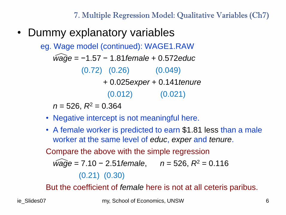
• Dummy explanatory variableseg. Wage model (continued): WAGE1.RAW
wage = −1.57 − 1.81female + 0.572educ
(0.72) (0.26) (0.049)
+ 0.025exper + 0.141tenure
(0.012) (0.021)
n = 526, R2 = 0.364
• Negative intercept is not meaningful here.
• A female worker is predicted to earn $1.81 less than a male
worker at the same level of educ, exper and tenure.
Compare the above with the simple regression
wage = 7.10 − 2.51female, n = 526, R2 = 0.116
(0.21) (0.30)
But the coefficient of female here is not at all ceteris paribus.
ie_Slides07 my, School of Economics, UNSW 6
7. Multiple Regression Model: Qualitative Variables (Ch7)
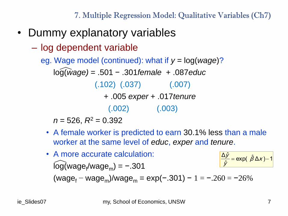
• Dummy explanatory variables
– log dependent variable
eg. Wage model (continued): what if y = log(wage)?
log(wage) = .501 − .301female + .087educ
(.102) (.037) (.007)
+ .005 exper + .017tenure
(.002) (.003)
n = 526, R2 = 0.392
• A female worker is predicted to earn 30.1% less than a male
worker at the same level of educ, exper and tenure.
• A more accurate calculation:
log(wagef/wagem) = −.301
(wagef − wagem)/wagem = exp(−.301) − 1 = −.260 = −26%
ie_Slides07 my, School of Economics, UNSW 7
1)Δˆexp(ˆ
ˆΔ xβ
y
y
7. Multiple Regression Model: Qualitative Variables (Ch7)
• Dummy explanatory variables
– Program evaluation
• To evaluate a social economic programs (eg. IT
training), individuals are divided into two groups:
a control or base group (nonparticipants) and a
treatment group (participants) .
• The outcomes (eg. wage) of the two groups can be
used to evaluate the program, using a multiple
regression model.
• A dummy variable represents the treatment group,
while other factors (eg. educ, exper) should be included
as controls.
• The coefficient of the dummy is the causal or ceteris
paribus effect of the program.
ie_Slides07 my, School of Economics, UNSW 8
7. Multiple Regression Model: Qualitative Variables (Ch7)
• Dummy variables for multiple categories
– What we do if individuals are from more than two
categories? (eg. gender-marriage, etc)
– In general, for g groups, we need g−1 dummy
variables, with the intercept for the base group.
– The coefficient on the dummy of a group is the
difference in the intercepts between that group and
the base group.
eg. (Wage model again) The base group is singmale :
wage = β0 + δ1 singfemale + δ2 marrfemale + δ3 marrmale
+ β1 educ + ... + u.
ie_Slides07 my, School of Economics, UNSW 9
many controls here
7. Multiple Regression Model: Qualitative Variables (Ch7)
• Dummy variables for ordinal information
– Consider a variable that takes multiple values, where
the order matters but the scale is not meaningful.
eg. A borrower’s credit rating is on the scale of 0-4 with
0=very risky, 1=risky, 2=neutral, 3=safe, 4=very safe.
– Use separate dummies for the multiple values.
eg. Credit rating dummies: with “very risky” as the base
group, cr1 = 1 if risky, cr2 = 1 if neutral, cr3 = 1 if safe,
cr4 = 1 if very safe.
– If an ordinal variable takes too many values, group
them into a small number of categories.
eg. Law school rankings: not sensible to use a dummy for
each value. Rather, use 5 dummies to indicate if the
rank is in the top 10, 11-25, 26-40, 41-60, rest.ie_Slides07 my, School of Economics, UNSW 10
7. Multiple Regression Model: Qualitative Variables (Ch7)
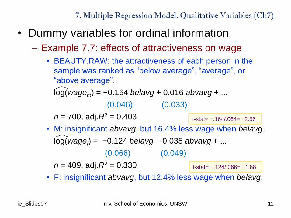
• Dummy variables for ordinal information
– Example 7.7: effects of attractiveness on wage
• BEAUTY.RAW: the attractiveness of each person in the
sample was ranked as “below average”, “average”, or
“above average”.
log(wagem) = −0.164 belavg + 0.016 abvavg + ...
(0.046) (0.033)
n = 700, adj.R2 = 0.403
• M: insignificant abvavg, but 16.4% less wage when belavg.
log(wagef) = −0.124 belavg + 0.035 abvavg + ...
(0.066) (0.049)
n = 409, adj.R2 = 0.330
• F: insignificant abvavg, but 12.4% less wage when belavg.
ie_Slides07 my, School of Economics, UNSW 11
t-stat= −.164/.064= −2.56
t-stat= −.124/.066= −1.88
7. Multiple Regression Model: Qualitative Variables (Ch7)
• Interactions among dummy variables
– Dummy variables can be interacted in the same way
as quantitative variables.
eg. (Wage model again) The base group is singmale :
wage = β0 + δ1 singfemale + δ2 marrfemale + δ3 marrmale
+ β1 educ + ... + u.
The dummies here are the interactions of two dummy
variables: female and married.
ie_Slides07 my, School of Economics, UNSW 12

7. Multiple Regression Model: Qualitative Variables (Ch7)
• Interactions among dummy variables
– Example 7.9 (Krueger,1993): the effect of computer
use on wage
log(wage) = .177 cwork + .070 chome + .017 cwork∙chome + ...
(.009) (.019) (.023)
• base group = those who do no use computers;
• 17.7% wage differential (over base group) for using a
computer at work (but not at home);
• 7% wage differential (over base group) for using a computer
at home (but not at work);
• 26.4% wage differential (over base group) for using a
computer at both home and work (exp(.177+.070+.017)-1 = .302);
• Interaction term is insignificant (t-stat = .017/.023 <1), meaning
that the effect of cwork is not linearly related to chome.
ie_Slides07 my, School of Economics, UNSW 13
other
factors
7. Multiple Regression Model: Qualitative Variables (Ch7)
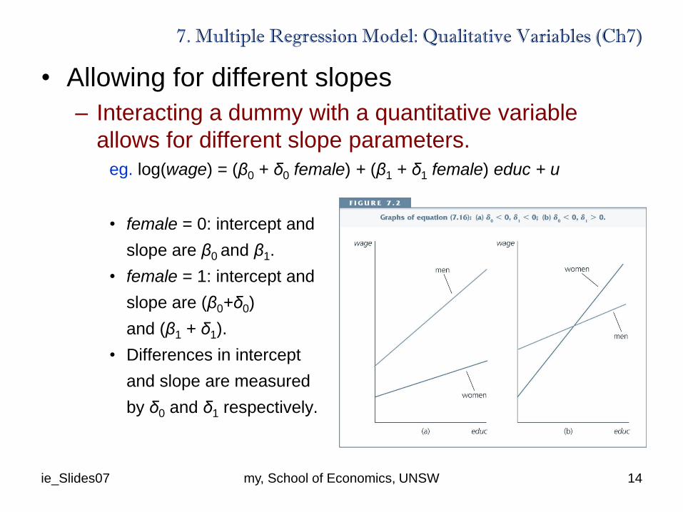
• Allowing for different slopes
– Interacting a dummy with a quantitative variable
allows for different slope parameters.
eg. log(wage) = (β0 + δ0 female) + (β1 + δ1 female) educ + u
• female = 0: intercept and
slope are β0 and β1.
• female = 1: intercept and
slope are (β0+δ0)
and (β1 + δ1).
• Differences in intercept
and slope are measured
by δ0 and δ1 respectively.
ie_Slides07 my, School of Economics, UNSW 14
7. Multiple Regression Model: Qualitative Variables (Ch7)
• Allowing for different slopes
– Interacting a dummy with a quantitative variable.
• (continued) To estimate, we use OLS for
log(wage) = β0 + δ0 female + β1 educ + δ1 female∙educ + u
where δ1 is the effect of the interaction of female and educ.
• A number of hypotheses of interest can be tested in this model.
a) the return to education is the same for men and women
(H0: δ1 = 0).
b) expected wages are the same for men and women
who have the same level of education
(H0: δ1 = 0 and δ0 = 0).
ie_Slides07 my, School of Economics, UNSW 15
7. Multiple Regression Model: Qualitative Variables (Ch7)
• Testing for differences in regression functions
across groups
– Different groups may have different coefficients. For
two groups (say f and m), the unrestricted model
involves 2(k+1) coefficients.
yf = βf,0 + βf,1 x1 + ... + βf,k xk + uf , and
ym = βm,0 + βm,1 x1 + ... + βm,k xk + um . (ur)
– Under the null hypothesis that there is no difference in
β coefficients across groups,
H0: βf,j = βm,j, j = 0, 1, ..., k,
the restricted model involves k+1 coefficientsis
y = β0 + β1 x1 + ... + βk xk + u . (r)
ie_Slides07 my, School of Economics, UNSW 16
7. Multiple Regression Model: Qualitative Variables (Ch7)
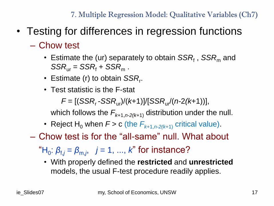
• Testing for differences in regression functions
– Chow test
• Estimate the (ur) separately to obtain SSRf , SSRm and
SSRur = SSRf + SSRm .
• Estimate (r) to obtain SSRr.
• Test statistic is the F-stat
F = [(SSRr -SSRur)/(k+1)]/[SSRur/(n-2(k+1))],
which follows the Fk+1,n-2(k+1) distribution under the null.
• Reject H0 when F > c (the Fk+1,n-2(k+1) critical value).
– Chow test is for the “all-same” null. What about
“H0: βf,j = βm,j, j = 1, ..., k” for instance?
• With properly defined the restricted and unrestricted
models, the usual F-test procedure readily applies.
ie_Slides07 my, School of Economics, UNSW 17
7. Multiple Regression Model: Qualitative Variables (Ch7)
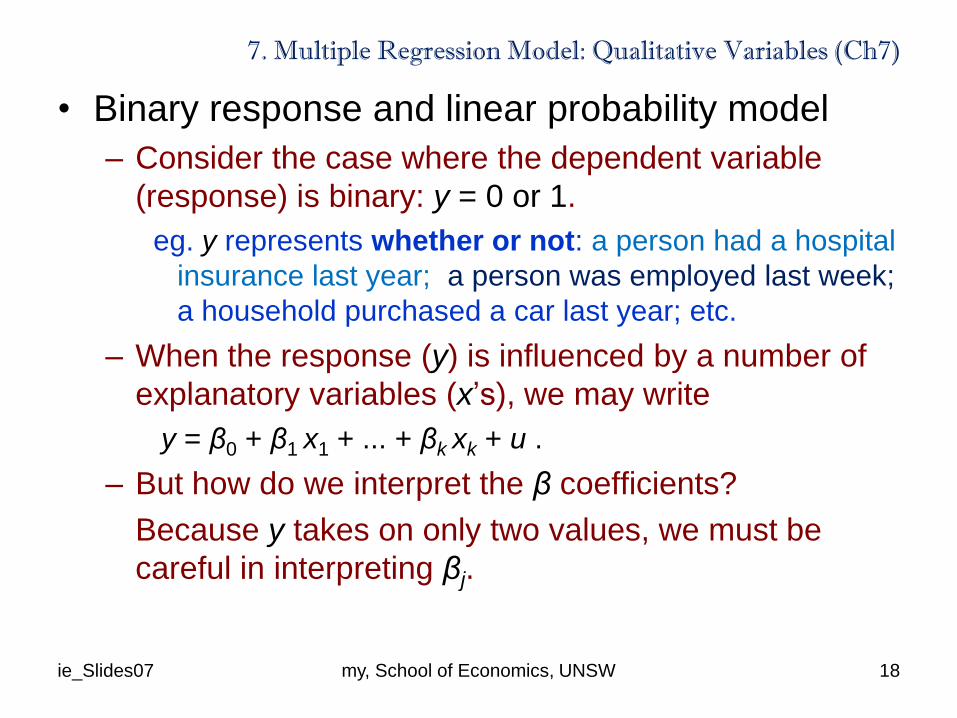
• Binary response and linear probability model
– Consider the case where the dependent variable
(response) is binary: y = 0 or 1.
eg. y represents whether or not: a person had a hospital
insurance last year; a person was employed last week;
a household purchased a car last year; etc.
– When the response (y) is influenced by a number of
explanatory variables (x’s), we may write
y = β0 + β1 x1 + ... + βk xk + u .
– But how do we interpret the β coefficients?
Because y takes on only two values, we must be
careful in interpreting βj.
ie_Slides07 my, School of Economics, UNSW 18
7. Multiple Regression Model: Qualitative Variables (Ch7)
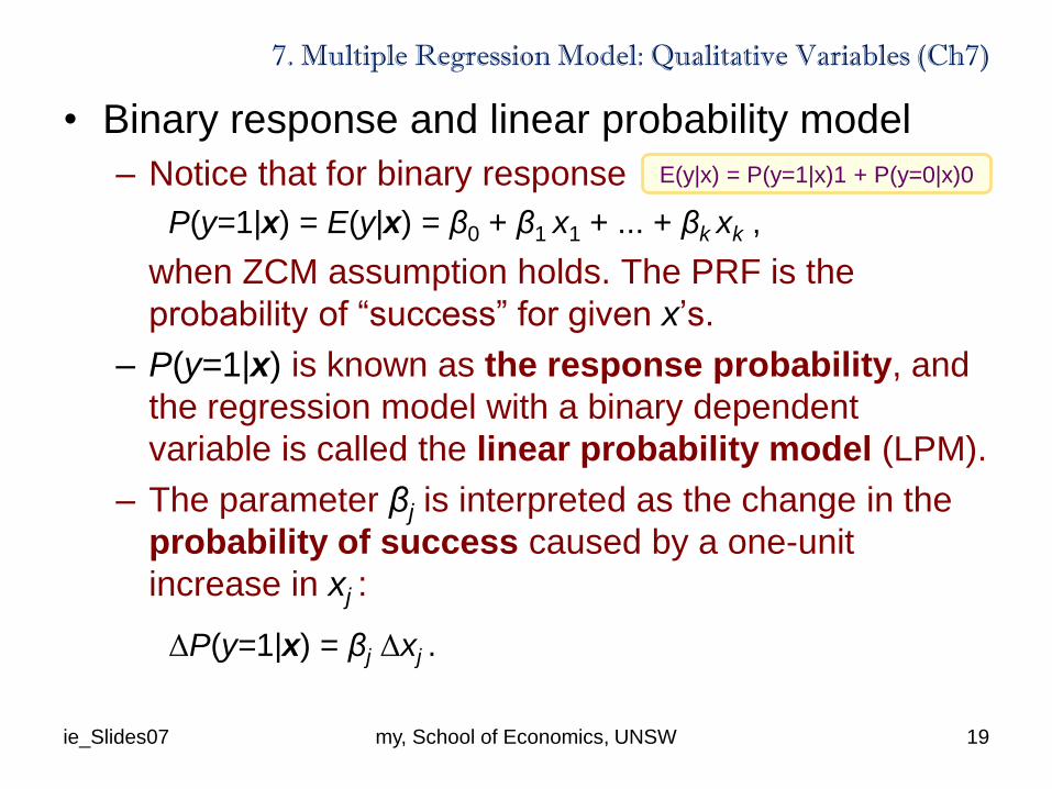
• Binary response and linear probability model
– Notice that for binary response
P(y=1|x) = E(y|x) = β0 + β1 x1 + ... + βk xk ,
when ZCM assumption holds. The PRF is the
probability of “success” for given x’s.
– P(y=1|x) is known as the response probability, and
the regression model with a binary dependent
variable is called the linear probability model (LPM).
– The parameter βj is interpreted as the change in the
probability of success caused by a one-unit
increase in xj :
ΔP(y=1|x) = βj Δxj .
ie_Slides07 my, School of Economics, UNSW 19
E(y|x) = P(y=1|x)1 + P(y=0|x)0
7. Multiple Regression Model: Qualitative Variables (Ch7)
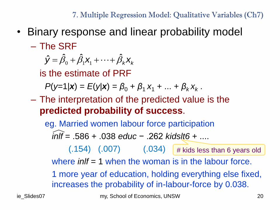
• Binary response and linear probability model
– The SRF
is the estimate of PRF
P(y=1|x) = E(y|x) = β0 + β1 x1 + ... + βk xk .
– The interpretation of the predicted value is the
predicted probability of success.
eg. Married women labour force participation
inlf = .586 + .038 educ − .262 kidslt6 + ....
(.154) (.007) (.034)
where inlf = 1 when the woman is in the labour force.
1 more year of education, holding everything else fixed,
increases the probability of in-labour-force by 0.038.
ie_Slides07 my, School of Economics, UNSW 20
kkxxy ˆˆˆˆ 110
# kids less than 6 years old

7. Multiple Regression Model: Qualitative Variables (Ch7)
• Binary response and linear probability model
– Shortcomings of LPM
• The predicted probability can be either less than 0 or
greater than 1. (eg. the in-labour-force probability for
those with kidslt6 ≥ 4 is predicted to be negative.)
– Linear function is not suitable for modelling probabilities.
– Logit model: P(y=1|x) = {1+exp[-(β0 + β1 x1 + ... + βk xk)]}-1
– Probit model: P(y=1|x) = Φ(β0 + β1 x1 + ... + βk xk)
• For LPM, it can easily be shown that
Var(u|x) = Var(y|x) = P(y=1|x)[1 − P(y=1|x)],
ie, MLR5 does not hold as the conditional variance
depends on x’s (heteroskedasticity). It does not cause
estimation bias but does invalidate the standard errors.
ie_Slides07 my, School of Economics, UNSW 21
7. Multiple Regression Model: Qualitative Variables (Ch7)
• Summary
– Dummy variables are useful to measure the ceteris
paribus differences among different groups in the
sample.
– Dummies are also useful to incorporate ordinal
information.
– Dummies can be interacted with other variables to
allow for different slopes for different groups, and
tests for various hypotheses of interest.
– Chow test and F-test are used to test for differences
in the regressions across groups.
– Binary response leads to the LPM, where the fitted
values are interpreted as probabilities of success.
ie_Slides07 my, School of Economics, UNSW 22