©idosr publications international digital organization for … · ©idosr publications...

www.idosr.org Okpara

180

IDOSR JOURNAL OF EXPERIMENTAL SCIENCES 2(1):180-228, 2017.

©IDOSR PUBLICATIONS

International Digital Organization for Scientific Research ISSN: 2579-0781

IDOSR JOURNAL OF EXPERIMENTAL SCIENCES 2(1):180-228, 2017.

Okpala Cyril Sunday

Impact of Financial Innovations and Demand for Money in Nigeria.

Department Of Economics, Ebonyi State University, Abakaliki

INTRODUCTION

The rising importance of financial sector in the economic development of

developing countries like Nigeria, as well as the rapid rate of innovation in that

sector have generated an increasing research interest in financial innovations and

the pattern of money demand. Gurley and Shaw (1960)[1] asserted that the paces of

economic development of any developing countries are greatly influenced by their

monetary conditions. In other words, a well functioning financial system is

inevitable for sustainable economic growth and development. There have been

immense developments in the banking sector, which lead to increase in branch

banking and use of information technology. The increase in branch banking in

Nigeria has occurred with the development of new technology to deliver services

such as Automated Teller Machines (ATMs) Electronic Funds Transfer, Credit Cards,

Debit Cards etc. These cost effective innovations and product that have become

available, have the purpose of reducing the pressure on overtime counter services to

bank customers.

Financial innovations may be defined as the emergence of new financial product or

services, new organizational forms or new processes for a more developed and

complete financial market that reduce cost and risks or provide an improved service

that meets customers‟ particular needs Bilyk (2002)[2]. The centrality of finance in a

modern economy and its importance in economic growth naturally raise the

requirement for financial innovations. A significant rationale for this research

derives from the Nigerian economic reforms beginning from the 80‟s but the

181 IDOSR JOURNAL OF EXPERIMENTAL SCIENCES 2(1):180-228, 2017.

inference from work shall spell implications of the most recent financial sector

reform.

The 2005 banks consolidation, exercise has changed the faces of banking in

Nigeria. The emergent 25 banks have new challenges to face: the challenge of inter

bank competition for customers and the challenges of new demands from their

customers. Banks customers now demand for varieties, convenience and new

services. They now want new services that can meet their individual needs. Also

technological availability in the past decade has helped banks to respond to these

challenges. Consequently, the transformation of the payment system for goods and

services through the use of transaction cards, e-banking etc would have a large

impact on the demand for cash and its role in the economy. The function of money

demand is considered to be among the central behavioural relationship in

macroeconomic theory. However, change in the structure of the financial sector can

objectively change the reliability of monetary policy.

According to Solans (2003)[3], the main reason for this is the presence of

financial innovations that introduce additional element of uncertainties to the

economic environment in which the central bank operates. Financial innovations

based on the following are necessary and useful element in forecasting money

demand. However, for the facts that financial innovation and demand for money

have not been empirically analyzed in Nigeria, informed the desired need to

undertake this research work “Financial innovation and demand for money in

Nigeria”.

STATEMENT OF THE PROBLEM

The rapid diffusion of financial innovations: Automated teller machines

(ATMs), credit cards, e-banking etc. Following the various economic reforms in the

country may have changed the pattern of money demand.

Some innovations may change the way in which the economy reacts to some

monetary policy or may affect information content of the indicators that the central

bank regularly monitor and that serve as a basis for taking policy decisions. Hence,


any analysis of money demand that do not account for these developments may

suffer from a potentially omitted variable problem.

Furthermore, financial innovation has raised serious problems in the

definition and measurement of money. This study seeks to replicate empirical works

carried out in the western world in Nigeria to see if financial innovation has had

significant effects in altering the demand for money in Nigeria.

There is and has always been considerable disagreement among economists

over what determines the levels and rates of growth of output, prices and

unemployment. The appropriate tool for macro economic stabilization depends on

the underlying theory in use. Keynesian, would go for fiscal policy while monetarists

would clamor for monetary policy.

Monetary policy refers to the use of interest rates, money supply and credit

availability to achieve macro-economic objectives. The use of monetary policy as a

tool for macro-economic stabilization depends largely on the behaviour of the

demand for money or real cash balances in the hands of economic agents. The

instability of the previously stable money demand for money function has thrown

up new studies at its various determinants and several other fronts have been

explored by economist and econometricians alike. One of these fronts is financial

innovations which has blurred the various definition, of money – m1

, m2

, m3

etc.

Also, the problem of estimating a stable money demand function has thrown

up a several lines of research.

RESEARCH QUESTIONS

This research work shall seek relevant answers to these posers otherwise

referred to as the research question such as:

1. To what extent will financial innovations impacts on demand for money in

Nigeria?

2. Is there any significant long run equilibrium relationship existing between

financial innovation and demand for money in Nigeria?

OBJECTIVES OF THE STUDY


The primary objective of this study is to appraise the effect of financial

innovations on demand for money in Nigeria.

However, specific objectives of the study which are to provide reasonable

answers to the research questions shall be:

1. To determine the impact of financial innovation on demand for money in Nigeria.

2. To determine if there is any long run equilibrium relationship existing between

financial innovations and demand for money in Nigeria.

RESEARCH HYPOTHESIS

This research shall be guided by the following hypothesis:

1. Financial innovation has no impact on demand for money in Nigeria.

2. There is no significant long run equilibrium relationship existing between

financial innovations and demand for money in Nigeria.

SIGNIFICANCE OF THE STUDY

In this era in Nigeria economy that have witnessed wide proliferation in

financial transactions technologies with various innovative ideas and instruments.

This research work is extremely important.

It shall be found very helpful in the following ways;

Since the effects of financial innovation, have never been investigated with

respect to money demand in Nigeria, the findings of this work/study shall add to

existing literature on money demand in Nigeria.

The knowledge of the impact of financial innovation on monetary aggregates will

also be useful in monetary policy implementation in Nigeria.

This study will also be helpful to the Central Bank of Nigeria (CBN) in monitoring

the movement of the monetary aggregates particularly with multiplicity of

transactions technologies brought about by the banking sector reforms.

Furthermore, members of the academic will find the study relevant as it will also

form basis for further research and a reference tell for academic work.

SCOPE AND LIMITATIONS OF THE STUDY


The study covers the growth and innovations in financial sector and has been

attested by financial innovations from the period of “1981 – 2014”. Though the

research would make reference to the related studies of other economies of the

world with a view of reviewing related literature on subject matter.

Data for this work shall be only on Nigeria economy. Such variables shall

include those related in existing literature to financial innovation and demand for

money. Data for this study shall be secondary, majorly from government owned

institution like the Central Bank of Nigeria (CBN).

REVIEW OF RELATED LITERATURE

THEORETICAL REVIEW

The relationship between the demand for money and its determinants is

considered as a fundamental issue in most theories of macroeconomic behaviour.

Stable function for money demand has long been seen as a critical component of

rational use of monetary aggregated in monetary implementation. Stable

relationship between money, real economy side variable and the set of assets

representing the opportunity cost of holding money is preconditioned in answering

the average growth-rate of money consistent with price stability[4].

Traditionally, most theories on the demand for money measure money

demand with the following are determinants:

i. Price level and rate of price change

ii. Income

iii. Interest

iv. Wealth

v. Rate of return on bonds and equities.

On the basis of theories, many authors have contributed to literature on the

estimation of money demand in the economy. Irvin Fisher, A.C Pigou, Jean Bodin, J.M

Keynes etc have all made their contribution to this topic.

QUANTITY THEORY OF MONEY


This is Irvin Fisher‟s formulation. In this formulation, money only serve as a

medium of exchange. He emphasized more on the transaction velocity of circulation

of money. In his analysis, he used the fact that in every transaction, there is a buyer

and a seller.

Thus, in aggregate total amount of sales must equal the amount of sales must

equal the amount of money in circulation multiplied by the average number of times

that it changes hand over that period. According to this theory, the amount of

money the economy needs to hold to facilitates transaction can be regarded as

bearing a fixed technical relationship to the level of money transaction.

CASH BALANCE THEORY

The Cambridge school represented by Alfred Marshal and A.C. Pigou took a

different approach. They diverted their analysis to the amount of money that an

individual wish to hold instead of the money an economy need to hold as fisher.

Money according to them could be held for its convenience in making

purchases and sales and also for security. The amount held being a function of the

volume of transaction and the returns available in alternative investment outlets in

form of interests and dividends, capital gains and losses. The principal determinant

of money holding by individuals is the fact that it is generally accepted in settlement

for goods and services. This means that the more transaction an individual has to

make, the more cash he would want to hold.

Apart from the level transaction, the demand for money varies with the level

of wealth, opportunity cost of holding money, income forgone by not holding other

assets, the price level and price expectations. They did not further work to establish

the relationship between these variables.

They argued that the demand for money by individuals, corporate bodies,

and the aggregates economy in nominal term is proportional to the nominal level of

income hence

Md = Kpy i.e. Md = Ms

Where:


Md = Quantity of money demanded

K = Constant Fraction of the value of all money transactions.

P = Prevailing price level

Y = Real output of goods and services

Ms = Quantity of money in circulation

This theory does not lay claim to the stability of money demand function but

did not make suggestion regarding the source of instability.

KEYNES LIQUIDITY PREFERENCE THEORY

In the Keynesian model, money becomes much more than a medium of

exchange, people demand money also for speculative purposes and as a security

against unforeseen needs for cash reserves. The transaction demand for money is

the need to hold money.

In this theory, the motive for holding money was broken down into three:

Transactionary demand, precautionary demand and speculative motive. The first

two depending on the level of income while the third (speculative) depends on

interest rate.

Keynesian model of money demand became a function of income and interest

rate i.e. md = L1

, (y) + L2

(r).

A major contribution of Keynes in this area is the explicit exposure of the

instability of money demand function. He attributed the instability to the vagaries of

speculative demand for money. While this position is expected, other factors other

than the vagaries of speculative demand for money may have contributed to the

instability. The theory thus postulates a stable demand for money function.

NIGERIA’S EXPERIENCE WITH FINANCIAL INNOVATIONS

Ever since the African banking corporation made it‟s debut on Nigeria

financial market in 1892, no time has there been such a massive deployment of

information technology as it is in the banking industry today; Forces often alluded

to this change were the wind of deregulation of banking industry in 1986 which

unleashed innovative and unprecedented competitive spirit among participants in


the sector. It was recognized though lately that information enable services could be

relatively efficient and cost effective than traditional face-to-face banking[5],[6].

Succinctly put, it is an enabler that defines and refocuses competition such

that its deployment in the right mix will alter quality and speed of service delivery.

No doubt, this underscores customer‟s paradigm shift, while in the past they were

contended with any services the banks preferred to offer; now they prescribe such

services. Now customers are unlikely to adopt and adapt to so called mall-produced

and mass marketing myopia, which characterized the pre-1986 banking period. Now

they want bank products and services that meet their specifications.

TRENDS IN FINANCIAL INNOVATION IN NIGERIA

The researcher took upon himself the duty of investigating the trend of

financial innovation to Nigeria through the construction of index of financial

innovation.

This index of financial innovation has been constructed similar to the one

developed by Holmes (2001)[7] and used by Bilyk (2006)[2]. First six major and most

frequently used financial innovation of the banking sector in Nigeria (e.g. ATM,

Credit card, Debit card, Wire transfer e-Banking). Secondly questionnaire on the

financial products and instrument was developed. Third, this questionnaire has been

distributed among top staff of Nigerian banks in order to determine the overall

development of financial innovations in Nigeria, the factors constitution, the

questionnaire have been treated equally.

The index has not been designed to measure the proportional contribution of

the set of statistically independent variable to development of Nigeria banking

during 1997 – 2006.

THE CASHLESS SYSTEM – AN OVERVIEW

Contrary to what is suggestive of the term, cashless economy does not refer

to an outright absence of cash transactions in the economic setting but one in which

the amount of cash-based transactions are kept to the barest minimum. It is an

economic system in which transactions are not done predominantly in exchange for


actual cash. It is not also an economic system where goods and services are

exchanged for goods and service (the barter system). It is an economic setting in

which goods and services are bought and paid for through electronic media. It is

defined as “one in which there are assumed to be no transactions frictions that can

be reduced through the use of money balances, and that accordingly provide a

reason for holding such balances even when they earn rate of return”. In a cashless

economy, how much cash in your wallet is practically irrelevant. You can pay for

your purchases by any one of a plethora of credit cards or bank transfer. Some

aspects of the functioning of the cashless economy are enhanced by e-finance, e-

money, e-brokering and e-exchanges. These all refer to how transactions and

payments are effected in a cashless economy.

In Nigeria, under the cashless economy concept, the goal is to discourage

cash transactions as much as possible. The CBN had set daily cumulative withdrawal

and deposit limits of N150,000 for individuals and N1,000,000 for corporate entities

(now reviewed to N500,000 and N3million respectively). Penalty fees of N100 and

N200 respectively (now reduced to 5% and 3% respectively) are to be charged per

extra N1000.

It should be said that as at now there are already some forms of cashless

transactions that are taking place in Nigeria. It is noted that: Today there are up to

seven different electronic payment channels in Nigeria, Automated Teller Machines

(ATM), points of sales terminals, mobile voice, web, inter-bank branch and kiosks. E-

payment initiatives in Nigeria have been undertaken by indigenous firms and have

been stimulated by improvement in technology and infrastructure. As noted above,

the cashless economy does not imply an outright end to the circulation of cash (or

money) in the economy but that of the operation of a banking system that keeps

cash transactions to the barest minimum. The CBN had set daily limits of cumulative

withdraws and lodgments of 150, 000 for individuals and 1,000,000 for corporate

customers (now 500,000 and 3million respectively). The operation of the system

does not mean the individual/corporations cannot hold cash in excess of 150,000/


N1million (now 500,000/N3million respectively) respectively at any single point in

time but that their cumulative cash transactions with the bank must not exceed

these limits over a period of one day. The system is targeted at encouraging

electronic means of making payments, and not aimed at discouraging cash holdings.

This policy on limits implies that an individual can actually have 5,000,000 (more

than 150,000 now 500,000) under his pillow at home, buys goods and services with

them but must not pay more than 500,000 into his bank in one day without

attracting a fine of 5% per 1000 for the excess. What is anticipated by this policy is

that instead of making large withdrawals to effect payment for goods and services,

such monies will be kept in the banking system so that payments are made through

“credit card-like means.” In this system users are issued with electronic cards which

can be slotted into special electronic machines in order to effect payments.

BENEFITS OF THE CASHLESS ECONOMY

Having seen how the system works, we would want to highlight the benefits

of the system. So much criticism has been raised about the cashless system. The

zenith of such criticism is that it has been labeled the “FORERUNNER OF THE MARK

OF THE BEAST”. However experts and government officials have continued to paint

the system in very colourful tones. For instance, the World Bank says that “operating

a cashless society in Nigeria was strategy for fast-tracking growth in the nation‟s

financial sector”. If the World Bank says so, one expects that to be true. Experts have

pointed out specific areas in which the cashless economy will enhance the quality of

life. These include:

1. Faster transactions – reducing queues at points of sales.

2. Improving hygiene on site – eliminating the bacterial spread through handling

notes and coins.

3. Increased sales.

4. Cash collection made simple – time spent on collecting, counting and sorting cash

eliminated.

5. Managing staff entitlements.


It is also noted that: It reduces transfer/processing fees, increases

processing/ transaction time, offers multiple payment options and gives immediate

notification on all transactions on customers‟ account. It is also beneficial to the

banks and merchants; (there) are large customer coverage, international products

and services, promotion and branding, increase in customer satisfaction and

personalized relationship with customers, and easier documentation and transaction

tracking. As a policy instrument, CBN has heaped a lot of praises on the cashless

system. CBN has hinged economic development on the cashless system; it sees it as

a tool for tackling corruption and money laundering. It has been pointed out that:

“Among the reasons glibly advanced by the CBN for this policy include reducing the

cost of cash management, making the Nigerian economy cashless, checking money

laundering and the insecurity of cash in transit”. Statistics show that cash

management in 2009 cost N114.5 billion and this is projected to stand at N200

billion in 2020. In the same vein, the cashless system provides the opportunity of

being able to “follow the money” and thus check money laundering across boarders.

Added to this is the perceived impact on the Naira. The system will reduce the

pressure on the Naira. This can only happen if there is effective and standard cross-

boarder electronic transmittal‟s reporting system. Following from the above

therefore, it is anticipated that the cashless system will bring with it transparency in

business transactions. In the same token, the cashless economy will bring with it a

leaning towards banking culture. It is seen that the effort is directed at ensuring

„cashless economy‟ and nurturing the culture of saving in the unbanked majority in

the country”. Most of Nigerians are still unbanked, and so we have large proportion

of the citizenry not subject to such monetary policy instruments as are used in the

banking system. This development will make CBN‟s policy tools more effective for

achieving economic development and stability goals.

EMPIRICAL LITERATURE

While the effect of financial innovations on demand for money has received

virtually no empirical attention in Nigeria. Some studies have been carried out to


determine the effect of financial innovation on demand for money elsewhere. These

studies have immensely contributed to the understanding of money demand

behaviour in the various countries where they were carried out. The findings of

these studies shall form the bulk of the empirical literature review of the current

work.

Nduka, Chukwu and Nwakaire (2013)[8] examine stability of demand for

money function in Nigeria for the period of 1986 to 2011. The study uses CUSUM

and CUSUMSQ tests for stability and reports that demand for money function is

stable during the period reviewed.

Adam, Kessy, Nyella and O‟Connell (2011)[9] study the demand for money

(M2) function in Tanzania using quarterly data from 1998Q1 to 2011Q4. The study

employs VAR and VEC approach. The variables employed are broad money demand

(M2), real GDP, interest rate, inflation rate and rate of nominal exchange rate

depreciation. The study reports that disaggregating currency and deposits, currency

responds more strongly to expected inflation, and deposits to the interest rate

spread vis-à-vis T-bills, than does overall M2. The results show the existence of a

stable cointegrating relationship between real money balances and its determinants

in Tanzania.

Halicioglu and Ugur (2005)[10] analyze the stability of the narrow money (M1)

demand function in Turkey with annual data of national income, interest rate, and

exchange rate for the period of 1950 to 2002. The study employs ARDL approach

with the CUSUM and CUSUMSQ for stability tests. The results show that there exists a

stable money demand function and suggests that it is possible to use the narrow

money aggregate as target of monetary policy in Turkey.

Similarly, Sovannroeun (2008)[11] estimates the demand for money function

in Cambodia with monthly data for the period of 1994:12 to 2006:12. The variables

used are demand for money balances proxied by M1, real income, inflation rate, and

exchange rate. The study employs ARDL approach of cointegration developed by

Pesaran. (1996, 2001) and CUSUM and CUSUMSQ tests for stability. The estimated


coefficient of error correction term indicates that there is cointegration among

variables in money demand function. The results also reveal that the estimated

elasticity coefficients of real income and inflation are respectively positive and

negative as expected. The exchange rate coefficient is negative which supports

currency substitution symptom in Cambodia. The study concludes that the demand

for money function is stable during the period covered in Cambodia.

In another study, Dritsakis (2011)[12] examines the demand for money in

Hungary using quarterly data for the period of 1995Q1 to 2010Q1. The study uses

the variables; money demand (M1), real income, inflation rate, and nominal exchange

rate. The study employs ARDL cointegrating framework and CUSUM and CUSUMSQ

stability tests. The results show that there is unique cointegrated and stable long-

run relationship among M1, real income, inflation rate, and nominal exchange rate.

Real income elasticity is positive, while the inflation rate elasticity and nominal

excahange rate are negative. The CUSUM and CUSUMSQ tests show that narrow

money demand function is stable over the period covered in Hungary.

Dagher and Kovanen (2011)[13] investigate the long-run stability of money

demand for Ghana with quarterly data for the period of 1990Q1 to 2009Q4. The

study Adopts ARDL approach and bounds test procedure developed by Pesaran.

(2001) and the CUSUM and CUSUMSQ tests for stability. The variables used are broad

money, real income, nominal effective exchange rate, domestic deposit interest rate,

the cedi treasury bill interest rate, the US treasury bill interest rate, and the US dollar

Libor interest rate. The results show that key determinants of money demand are

real income and exchange rate, while other financial variables are found

insignificant in the estimation. The study reports a stable long-run money demand

function in Ghana.

In a similar study, Baba, Kenneth and Williams (2013)[14] examine the

dynamics of money demand in Ghana with annual data for the period of 1980 to

2010. The study employs Dynamic Ordinary Least Squares (DOLS). The variables

used are narrow money demand, GDP as a proxy for income, consumer price index


and, nominal exchange rate. The results show that apart from income, inflation and

exchange rate elasticities are negative. The study reports a stable money demand

function, and concludes that changes in past and current macroeconomic activity

significantly affect money demand in Ghana.

In other studies conducted on Indian economy, Das and Mandal (2000)[15]

considers M3 money supply and conclude that money demand function is stable in

India. The study uses monthly data for the period of April 1981 to March 1998. The

variables used are industrial production, short-term interest rates, wholesale prices,

share prices, and real effective exchange rates. The results show that there is

cointegrating vectors among M3 and the other variables.

In contrast, Inoue and Hamori (2008)[16] empirically analyze India‟s money

demand function for the period of 1980 to 2007 with both monthly and annual data

for the period from 1976 to 2007. The study employs dynamic OLS (DOLS) and

carries out cointegration tests. The variables used are real demand for money

balances (M1, M2, and M3) as dependent variable, interest rates and output as

independent variables. The results show that when money supply is represented by

M3, there is no long-run equilibrium, whereas there is long-run equilibrium when

money supply is represented by M1 and M2 and the coefficients of interest rate and

output are consistent with economic theory, respectively.

Hamori (2008)[17] analyzes the demand for money function in 35 Sub-

Saharan African countries including Nigeria, for the period of 1980 to 2005 and

adopts a non-stationary panel data analysis. The variables used are real money

balances (M1); real money balances (M2); real GDP; interest rate, and inflation rate.

The empirical results reveal that that there exists a cointegrating relation with

respect to money demand in the Sub-Saharan African region over the period studied,

regardless of whether M1 or M2 is used as the money supply measure. Thus, money

supply (M1 and M2) is a reliable policy variable from the intermediate-target

perspective.


In a similar study on eleven Euro countries, Hamori and Hamori (2008)[18]

reveal that the money demand fuction is stable with respect to M3 money demand in

Euro aria. The results of the panel estimation indicate that the output coefficient is

positively related to M3, while the interest rate is negatively related to M3 in the

eleven Euro countries. Felmingham and Zhang (2000)[19] investigate the long-run

demand for broad money in Australia subject to regime shifts with monthly data

over the period of 1976(3) to 1998(4). The study employs Gregory Hansen

cointegration. It reveals some evidence for the presence of cointegration between

broad money, non-money assets, and GDP. The results show a break date in 1991

coinciding with a deep recession and policy induced interest rate reductions in

Australia during the period. The income elasticity of demand exceeds one,reacts

positively to the interest spread and negatively to inflation.

Lungu, Simwaka, and Chiumia (2012)[20] study the demand for money

function in Malawi using monthly data for the period of 1985 to 2010. The variables

used are real money balances, prices, income, exchange rate, treasury bill, and

financial innovation. The study employs VAR, VEC, and Granger causality

approaches. The results show that the model is stable and adequate. It further shows

that in the long-run real GDP, inflation, exchange rate, treasury bill rate, and

financial depth all have significant impact on the demand for money, while in the

short-run, it is financial innovation, exchange rate movements, and lagged money

supply that display causality in money demand.

Suliman and Dafaalla (2011)[21] investigate the existence of a stable money

demand function in Sudan using annual data for the period of 1960 to 2010. They

employ the Johansen Maximum Likelihood procedure using real money balances,

real GDP (as a scale variable), the rate of inflation and exchange rate (as opportunity

cost of holding money balances variables). All variables are in logarithmic form,

except inflation rate. The results reveal that there is a long-run relationship between

real money balances and the explanatory variables. The study further shows that

money demand function is stable between 1960 and 2010 in Sudan. The study


concludes that it is possible to use the narrow money aggregate as target of

monetary policy in Sudan.

Similarly, Dahmardeh, Pourshahabi, and Mohmoudinia (2011)[22] empirically

study the long-run relationship between money demand and its determinants in Iran

with annual data for the period of 1976 to 2007. The study employs conditional

ARDL model with economic uncertainty, money demand, real income, and real

interest rate as the variables. The results show that economic uncertainty has a

significant negative effect on money demand; real income has a positive and

significant effect on money demand, while interest rate has a negative effect on

money demand. Moreover, economic uncertainty measured by EGARCH (1,1) model

of inflation rate, exchange rate, growth of GDP and terms of trade, has a negative

and significant effect on money demand in Iran. The study, therefore reports that

there exists a long-run relationship between M1 and its determinants in Iran.

Anoruo (2002)[23] investigates the stability of demand for money in Nigeria

during the SAP period. Results from Johansen and Juselius (1990)[24] cointegration

tests show that real broad money, economic growth, and real discount rate have a

long-run relationship. The study employs Adebiyi (2006)[25] stability test and

reports that demand for broad money is stable in Nigeria during the SAP period from

1986Q2 to 2000Q1.

In another study, Akinlo (2006)[26] examines the cointegrating property and

stability of M2 money demand in Nigeria. The results reveal that M2 is cointegrated

with income, interest rate and exchange rate. Moreover, the results show that income

is positively related to demand for money, while interest rate is negatively related to

demand for money.

Nwafor (2007)[27] examine the quantity theory of money via Keynesian

liquidity preference theory in Nigeria using quarterly data from 1986Q3 to 2005Q4.

The variables used are demand for money (M2), real income, real interest rate, and

expected inflation rate. The study employs the ADF unit root and Johansen-Juselius

cointegration tests. The results show that demand for money is positively related to


real income, real interest rate, and expected inflation rate, respectively in Nigeria.

The study therefore concludes that there exists a longrun relationship among

aggregate demand for money in accordance with the Keynesian liquidity preference

theory.

Gbadebo (2010)[28] examines whether financial innovation affects the

demand for money in Nigeria for the period from 1970 to 2004. The study employs

OLS and Engle-Granger cointegration techniques. The variables used are broad

money, nominal interest rate on time deposit, real GDP, nominal rate on treasury

bills, dummy variable to capture SAP period, consumer price index and lag of broad

money. The results suggest that financial innovations have not significantly affected

the demand for money in Nigeria during the period studied.

Omanukwue (2010)[29] investigates the modern quantity theory of money

with quarterly time series data from Nigeria for the period of 1990Q1 to 2008Q4.

The study employs Engle- Granger two-stage approach for cointegration to examine

the long-run relationship between money, prices, output, interest rate and ratio of

demand deposits/time deposits. It employs also the granger causality to examine the

causality between money and price. The study establishes the existence of

weakening uni-directional causality from money supply to core consumer prices in

Nigeria. The study also reports evidence of a long-run relationship between the

variables. In all, the results indicate that monetary aggregates still contain

significant, albeit weak, information about developments in core prices in Nigeria.

Kumar, Webber and Fargher (2010)[30] investigate the level and stability of

money (M1) demand in Nigeria for the period of 1960 to 2008 with annual data. In

addition to estimating the canonical specification, alternative specifications are

presented that include additional variables to proxy for the cost of holding money.

Results of Gregory-Hansen cointegration tests suggest that the canonical

specification is well determined. The money demand relationship went through

regime shift in 1986 and 1992 respectively, which slightly improved the scale of

economies of money demand. The results further show that there is a cointegrating


relationship between narrow money, real income and nominal interest rate after

allowing for a structural break. The study concludes that the demand for money was

stable in Nigeria between 1960 and 2008 although there is evidence to suggest that

it may have declined by a small amount around 1986.

Similarly, Chukwu, Agu and Onah (2010)[31] examine the evidence in the

money demand function in the structural break framework with unknown break

point for the period of 1986Q1 to 2006Q4 in Nigeria. The variables used are real

money demand (M2) as dependent variable, real income, interest rate proxied by

interest swap spread, and expected rate of inflation proxied by CPI as independent

variables. The study employs the Gregory-Hansen approach for cointegration. The

results show that real income and interest rate are positively related to real demand

for money, whereas expected rate of inflation is inversely related to money demand.

The results further show that there exists structural breaks in the cointegrating

vectors of the Nigerian long-run money demand

function in 1994, 1996, and 1997.

Omotor (2011)[32] estimates an endogeneous structural break date of the

money demand for Nigeria for the period from 1960 to 2008 with Gregory- Hansen

cointegration approach. The variables employed are broad money, real GDP and

nominal interest rate. The results suggest that there exists a stable long-run demand

for money function in Nigeria during the period reviewed.

Bitrus (2011)[33] examines the demand for money in Nigeria with annual data

on both narrow and broad money, income, interest rate, exchange rate, and the stock

market for the period of 1985 to 2007. The study employs OLS technique and

CUSUM stability test. The results show that money demand function is stable in

Nigeria for the sample period and that income is the most significant determinant of

the demand for money. It further shows that stock market variables can improve the

performance of money demand function in Nigeria.

Similarly, Bassey (2012)[34] investigate the effect of monetary policy on

demand for money in Nigeria with annual data for the period of 1970 to 2007. The


study employs OLS multiple regression technique and finds inverse relationship

between money, domestic interest rate, expected rate of inflation and exchange rate.

Watson (2001)[35] studies the demand for money in Jamaica with quarterly

data from 1976Q1 to 1998Q4. The study employs both restricted and unrestricted

VAR models and structural cointegration. The variables used are money supply,

national income, deposit price level, rate of interest, base money, deposit rate of

interest and, interest on loans. The results show that there exists a stable long-run

demand for money function in Jamaica over the period studied. The study concludes

that the Error Correction form had satisfactory diagnosis while the Persistence

Profiles, a useful tool for policy analysis purposes, are not at odds with the

predictions of economic theory.

Nachega (2001)[36] applies VAR models analysis to investigate the behaviour

of demand for money (M2) in Cameroon from 1963/64 to 1993/94. The cointegrated

VAR analysis first describes an open-economy model of money, price, income, and a

vector of rates of return, within which three steady state relations are identified: a

stable money demand function, an excess aggregate demand relationship, and the

uncovered interest rate relation under fixed exchange rates and perfect capital

mobility. The results show a short-run stable demand for money in Cameroon over

the period studied.

Bilyk (2006)[2] in his thesis “Financial innovation and demand for money in

Ukraine” Using Ukrainian data between 1997 – 2005 made the assertion that failure

to model financial innovation in money demand functions may yield unstable and

mis-specification of functions.

Hester, Calcagnini and De Bonis (2001)[37], using data between 1991 and

1995 for 6 sample of large Italian banks find some evidence supporting the idea that

ATMs reduce transaction cost and demand currency.

Blankson and Belnye (2004)[38] in their paper “The impact of financial

innovation and demand for money in Ghana” modeled money demand function to

include two different proxies for financial innovations: volume of cash cards


transaction and the ratio of m2

to m1

(i.e. m2

/m1

). Their result showed that there is a

long run positive impact of financial innovation in demand for money in both cases.

The results using ECM showed that changes in innovation enter the demand for

money with significant and positive signs. This means that changes in innovations

exert a positive influence on demand for narrow money. Hence, increase in

innovation leads to an increase in the demand for narrow money in an economy.

Bilyk (2001)[2] found positive relationship, between financial innovation and

demand for money in Ukraine. The study period covers nine years from January

1997 till December 2005. The empirical part of the thesis was conducted by means

of error – correction model (UECM).

Bacao (2001)[39] estimated and tested an econometric model of demand for

narrow money in Portugal. The error correction model was based on adjusted

velocity of circulation. The timing of the shifts in the velocity of circulation does not

appear to be relate financial innovation. Hence Bacao concluded that financial

innovation though theoretically has some influence on demand for but its effect is

not observable to warrant empirical investigation.

Emmanuel (2002)[40] examined the stability of the m2

money demand

function in Nigeria in the Structural Adjustment Programme (SAP) period. The result

from the Johansen and Juselius Co integration test suggests that real discount rate,

economic activity and real m2

was co integrated.

Busart (2004)[41] using co integration and error correction approach on

annual data for the period of 1970 – 2003 to examine Nigeria money demand

function. In this study, he observed that demand for money in Nigeria this was

stable and that reforms measures introduced in the mid 1980s seems not to have

significantly altered the demand function for money in Nigeria.

Adebiyi (2006)[25] examined broad money demand, financial liberalization

and currency substation in Nigeria using Error Correction Model (ECM). His result

showed that long run demand for real balances in Nigeria depends upon real income

on its own interest rate on government securities, inflation and expected exchange


rates. He finally concluded that money demand function in Nigeria was stable

despite the economic reforms and financial crises.

Gibadepo and Adedapo (2008)[42] examined the impact of financial innovation

on the stability of Nigeria money demand function using Johanson ECM and they

found that financial innovation has impact but not a significant impact

In summary, the above empirical review indicates that most of the works

mentioned were studies of other countries. Those of Nigeria were either weak due to

fewer numbers of years covered in the study or suffer from inadequacies that the

study extends its scope to 2014 from 1981.

RESEARCH METHODOLOGY

RESEARCH DESIGN AND METHODOLOGY

The research design to be employed in this work is the ex-post facto or

multiple regression method, based on ordinary least square. The choice for the ex-

post facto stems from its major objective which is to explore the relationship

between financial innovations and demand for money in Nigeria. The Ex-post facto

methodology is considered most appropriate for a research of this sort for the

following reasons: This research design tries to dig out the cause and effect

relationships where causes already exists and cannot be manipulated. The ex-post

facto or causal comparative research design makes use of what already exists and

looks backwards to explain why it is so and. It provides a means to measure the

effects of the independent variables on the dependent variable.

Multiple regressions involving the ordinary least square method of estimation

shall be employed in this research.

The choice of this method is based on the “BLUE” property that is Best Linear

Unbiased Estimation. This is because it helps to ascertain quantitatively the impact

of certain factors on a given phenomenon under study. According to Koustsyianis

(1977) states that in attempting to study any relationship between variables, it is

important to express the relationship in mathematical form.


MODEL SPECIFICATION

The model specification will be

DM = F (FI, INT, LR) (1)

Where;

DM is the demand for money

FI is financial innovations

INT is interest rate

LR is the liquidity ratio.

DM, demand for money is the dependent variables while financial innovation;

interest rate and liquidity ratio are the independent variables. To show the impact

financial innovations and demand for money in Nigeria of will be,

DM = βO

+ β1

FI+ β2

INT+

β3

LR + Ut

(2)

Where Ut are those variables that can affect the DM which are not stated in

the model specification.

ESTIMATION PROCEDURE

Prior to running a regression to obtain the ordinary least square (OLS)

estimates and the non linear component of the system using the state space model

(SSM), the entire series shall be subjected to some econometric and deterministic

examinations.


UNIT ROOT TEST

The unit root test is utilized to test for the stationary of time series data.

Since most of the macroeconomic time series are non-stationary (Nelson and Plosser,

1982) and are prone to spurious regression, the first step in any econometric or time

series analysis is always to test for stationary. The widely used augmented dickey

fuller (ADF) test statistic shall be used to test for stationarity. It shall be compared

with the critical values at 5% level of significance. If the ADF test statistic is at any

level, greater than the critical values with consideration on their absolute values, the

data at the tested order is said to be stationary. Augmented Dickey-fuller test relies

on rejecting a null hypothesis of stationary. The tests are conducted with and

without a deterministic trend (t) for each of the series. For the purpose of this

research, an augmented dickey-fuller (ADF) test shall be conducted by carrying out a

unit root test based on the following structure: s

∆xt

= k + at

+ θxt

-1

+ ∑t=I

Φ∆t

-1

+ et

(3)

Where X is the variable under consideration, ∆ is the first difference operator, t

captures time trend, at is a random error, and n is the maximum lag length. The

optimal lag length is identified so as to ensure that the error term is white noise. K,

a, θ and Φ are the parameters to be estimated. If we cannot reject the null hypothesis

that θ=o, then we conclude that the series under consideration has a unit root and is

therefore non-stationary. On the assumption of unit root for all the variables

employed, we would proceed to test for co integration.

CO INTEGRATION TEST

The whole series shall at this stage be tested for co integration to further

ensure that the entire model is not spurious. A series is co integrated if all the

variables in the model present a unit root or are stationary even if one or all the

variables are individually non stationary (Gujarati, 2009)[43]. Granger (1969)[44],

recommends the test for co integration when he noted that tests for co integration

are pre tests to avoid spurious regression situations. If dependent and independent

variables are co integrated according to Gujarati (2009)[43], the implication is that


there exists a relationship between the short and long run equilibrium. The co

integration test is useful in determining if there is any long run relationship between

the variables in model. The focal point of this study shall be to know if a long run

equilibrium relationship exists between financial innovations and demand for

money in Nigeria. The econometric framework used for analysis in this study is the

Johansen (1998) and Johansen and Juselius (1990)[45],[24] maximum likelihood co

integrating vectors. This multivariate co-integration test can be expressed as:

Z t

= k1

zt

-1

+ k2

zt

-2

+ …….…… + kk

-1zt

-k

+ ut

+ vt

(4)

Where zt (DM, FI, INT and LR) is an nx

1 vector of the variables, DM, FI, INT and LR

are

proxy representing demand for money, financial innovation, interest rate and

liquidity ratio respectively. The constant vector is represented by ut

while vt

is a

vector of normally and independently distributed error term. To determine the

number of co-integrating vectors, Johansen developed two likelihood ratio tests:

trace test (λtrace) and maximum eigenvalue test (λmax). This study shall depend on

the trace statistic in taking decisions about the number of co integrating vectors. If

co integrating vector(s) is or are identified, we proceed to develop and estimate

vector error correction model (VECM).

VECTOR AUTO REGRESSION (VAR)

The Vector Autoregression (VAR) model is one of the most flexible and

effective models for the examination of multivariate time series. The VAR model was

presented into practical econometrics by Koutsoyiannis (1977)[46]. It is a natural

generalisation and an addition of the nivariate autoregressive model to dynamic

multivariate time series. The vector autoregression (VAR) model has confirmed to be

very valuable for forecasting and for describing the dynamic behaviour of economic

variables and financial time series and for forecasting. It often offers better

forecasts than those from univariate time series models. In general, the VAR models

can be made conditional on potential future paths of specified variables and are

often seen to provide a more flexible forecast. Additionally, in order to provide data

description and forecasting, the VAR model could be employed for policy analysis


and structural inference. Typically, the imposition convinced assumption about the

causal structure of the data under investigation is vital to summarize the causal

effects of innovations and unforeseen shocks on the variables in the model.

SOURCES OF DATA

Data is obtained from secondary sources. All the variables to be employed in

the empirical estimation and analysis shall be sourced from various issues of the

Central Bank of Nigeria.

PRESENTATION AND ANALYSIS OF RESULTS

The attempt to study the impact of financial innovations and demand for

money in Nigeria led the researcher to subject the data collected to Unit Root, Co

integration, and Vector Auto Regression VAR Test. The variables considered in this

research work are: Demand for money (DM) (dependent variable) and the

independent variables include: financial innovations (FI), interest rate (INT) and

liquidity ratio (LR). The empirical results are presented below:

UNIT ROOT TEST

In other to test for the presence or absence of unit root in the data used for

the empirical analysis, Augmented Dickey-Fuller (ADF) test was employed and the

test result is as presented below:

TABLE1: AUGMENTED DICKEY FULLER UNIT ROOT TEST AT LEVEL (TREND AND

INTERCEPT)

Variables ADF @

Level

1st

difference

2ND

Difference

Critical

value

(5%)

Critical

value

(10%)

Order of

integration

Remarks

D(DM) -

0.600702

-5.424532 - -

4.273277

-

3.557759

I(1) Stationary

D(FI) -

2.216232

-5.294050 - -

4.273277

-

3.557759

I(1) Stationary

D(INT) -

2.992615

-6.036610 - -

4.284580

-

3.562882

I(1) Stationary

D(LR) -

3.179814

-6.057269 - -

4.273277

-

3.557759

I(1) Stationary

SOURCE: Researcher own compilation

From the result above, all the variables, that is, Demand for money (DM),

Financial innovations (FI), Interest rate (INT) and Liquidity ratio (LR) exhibited


stationarity at first difference. The stationarity is achieved by comparing their

respective ADF test statistics with the 5% critical values; it is observed that their

respective test statistics are greater than the critical values in absolute terms. Thus,

the series are stationary.

CO-INTEGRATION RESULT

To test for the presence of long run relationship among the variables, the

researcher adopted the econometric method of Johansson co integration and the

result from the test is shown in the table below.

Series: LDM LFI INT LR

Lags interval (in first differences): 1 to 2

Unrestricted Cointegration Rank Test (Trace)

Hypothesiz

ed

Trace 0.05

No. of

CE(s)

Eigenvalue Statistic Critical

Value

Prob.**

None 0.497912 40.43526 47.85613 0.2073

At most 1 0.294089 19.07690 29.79707 0.4874

At most 2 0.210651 8.280625 15.49471 0.4359

At most 3 0.030108 0.947695 3.841466 0.3303

Trace test indicates no cointegration at the 0.05 level

The results of the co-integration in the table above indicated that the trace statistics

is lesser than the critical value at 5 percent level of significance in all of the

hypothesized equations. This confirms that there is no cointegration relationship

among the various variables used to model the relationship between financial

innovations and demand for money in Nigeria for the period under investigation.

Specifically, the results of the cointegration test suggested Demand for money (DM)

had equilibrium relationship with Financial innovations (FI), Interest rate (INT) and

Liquidity ratio (LR) which kept them in equilibrium to each other in the short run.

Also, its Eigenvalue was insignificantly lesser than one.

The normalized co-integrating coefficients for 1 cointegrating equation given by the

short run relationship is

DM = -0.824094F1 + 0.663738INT + 0.302255LR


Where demand for money (DM) is the dependent variable, -0.824094 is the

coefficient of financial innovations (FI), 0.663738 is the coefficient of interest rate

(INT) and 0.302255 is the coefficient of liquidity ratio (LR). The sign borne by the

adjusted coefficient estimates of FI is negative, while INT and LR is positive. This

implies that in the short run, the relationship that will exist between FI and GDP will

be negative, while INT, LR and GDP will be positive.

VECTOR AUTO REGRESSION (VAR)

The Vector Auto regression (VAR) model is one of the most flexible and

effective models for the examination of multivariate time series. The VAR model was

presented into practical econometrics Nelson and Plosser (1982)[47]. It is a natural

generalisation and an addition of the nivariate autoregressive model to dynamic

multivariate time series. The vector auto regression (VAR) model has confirmed to be

very valuable for forecasting and for describing the dynamic behaviour of economic

variables and financial time series and for forecasting. It often offers better

forecasts than those from univariate time series models.

Vector Autoregression Estimates

Date: 11/08/16 Time: 01:45

Sample (adjusted): 1982 2014

Included observations: 33 after adjustments

Standard errors in ( ) & t-statistics in [ ]

LDM

LDM(-1) 0.910003

(0.11367)

[ 8.00539]

LFI(-1) 0.055421

(0.09463)

[ 0.58569]

INT(-1) 0.050430

(0.01985)

[ 2.53997]

LR(-1) 0.006295

(0.00788)

[ 0.79863]

C -0.689861

(0.48977)


[-1.40855]

Source: Own Computation (See Appendix)

R2

= 0.979195

The result is significant since the coefficient of multiple (0.979195)

determination is greater than zero. From the result of the estimation using VAR Test

presented above, the coefficient of the constant term is -0.689861 implying that

when other variables are kept constant demand for money (DM) decreased by

0.689861 units. The coefficient of FI(-1) is 0.055421 implying that a unit change in

financial innovations brought about a 0.055421 unit increase in DM. Similarly, the

coefficient of INT is 0.050430 implying that a unit change in interest rate brought

about a 0.050430 unit increase in DM. At the same time, LR has a coefficient of

0.006295, meaning that a unit increase in liquidity ratio brought about a 0.006295

unit increase in DM.

The above result indicates that the R2 is 0.979195 indicating that the

explanatory variables explain about 97.91% of the total variations in DM during

the period under consideration while other variables not captured in the model

accounted for about the remaining 2.09 percent.

TEST OF HYPOTHESES

HYPOTHESES ONE

Ho:

There is no long run relationship between financial innovations and demand

for money in Nigeria.

H1:

There is long run relationship between financial innovations and demand for

money in Nigeria.

To test the null hypothesis stated above, the researcher made use of the

Johansson Cointegration analysis and the result is presented below.


Hypothesiz

ed

Trace 0.05

No. of

CE(s)


Value

Prob.**

None 0.497912 40.43526 47.85613 0.2073


At most 1 0.294089 19.07690 29.79707 0.4874

At most 2 0.210651 8.280625 15.49471 0.4359

At most 3 0.030108 0.947695 3.841466 0.3303


The results of the co-integration in the table above indicated that the trace statistics

is lesser than the critical value at 5 percent level of significance in all of the

hypothesized equations. This confirms that there is no cointegration relationship

among the various variables used to model the relationship between financial

innovations and demand for money in Nigeria for the period under investigation.

Specifically, the results of the cointegration test suggested Demand for money (DM)

had equilibrium relationship with financial innovations (FI), Interest rate (INT) and

Liquidity ratio (LR) which kept them in equilibrium to each other in the short run.

Also, its Eigenvalue was insignificantly lesser than one. In other words, the null

hypothesis of no cointegration among the variables is accepted.

HYPOTHESES TWO

Ho

: Financial innovations do not impact on demand for money in Nigeria.

H1

: Financial innovations do impact on demand for money in Nigeria.

From the relationship existing between financial innovations and demand for

money in Nigerian as was revealed by the VAR analysis, we observed that there is a

positive relationship between financial innovations and demand for money and as

such we reject the null hypothesis and conclude that financial innovations do impact

on demand for money in Nigeria.

IMPLICATION OF THE STUDY

The VAR result indicated that there was a positive relationship between

financial innovations and demand for money. This does conform to a priori

expectation. A positive relationship was expected to exist among financial

innovation and demand for money. Hence the positive relationship between

financial innovations and demand for money could be attributed to the fact that

government in recent years had employ more resources into the financial sectors

leading to substantial development which tends to impact in the country‟s general


development and also fostering international partnership with other countries.

Interest rate and liquidity ration from the results showed that they

had no impact on

DM compared to FI and as such, it is advised that interest rate of financial sectors

should be lowered in other to increase the amount of money or loan demanded by

investors for substantial development in the financial sector and the economy at

large. The analysis also shows that for the atmosphere to be conducive for the

effective use of monetary policies, financial innovations should be made to affect

the demand for money significantly; there is still a place for monetary policy as a

macroeconomic stabilization measure. The implication of the result is that an

increased financial innovation in conjunction with lowered interest rate and liquidity

ratio will continue to improve the Nigerian economy[48].

SUMMARY, CONCLUSION AND RECOMMENDATION

SUMMARY OF FINDINGS

The study investigated empirically the relationship between financial

innovations and demand for money in Nigeria for the period between 1981 and 2014

employing various techniques of econometric analysis. In the course of the study,

the main objective was to investigate the impact of financial innovations and

demand for money in Nigeria for the period under review. The variables used for the

empirical analysis in this study are; demand for money (DM), financial innovations

(FI), interest rate (INT) and liquidity ratio (LR).

On the application of advanced econometric techniques (Augmented Dickey

Fuller, Johansen Cointegration Test, and Estimation of Toda-Yamamoto using VAR

Test), the following information were extracted;

All the variables (DM, FI, INT and LR) became stationary at first difference

using augmented dicey fuller unit root test application; this means they all

have unit roots which necessitates the application of Johansson cointegration

test to test for long run relationship.

The cointegration result indicated that the variables had short run

relationship with no cointegrating equations. Hence, there exists a short-run


equilibrium relationship between financial innovations and demand for

money in Nigeria.

To ascertain the impact of financial innovations and demand for money in

Nigeria, the study made use of Vector Auto Regression Test. From the result

of the VAR presented above, there exist a positive relationship between

demand for money (DM), financial innovations (FI), interest rate (INT) and

liquidity ratio (LR). The positive relationship between DM and FI does

conform to a priori expectations.

Finally, the regression result indicated that the coefficient of determination (R2

) was

0.979195. This indicates that the explanatory variables explain about 97.91% of

the total variations in GDP during the period under consideration while other

variables not captured in the model accounted for about the remaining 2.09

percent.

CONCLUSION

This study has looked at the demand for money and how it has been affected

by financial innovations in the financial sector of Nigeria arising out of the

Structural Adjustment Programme (SAP) of 1986. The term financial innovation

refers to anything which ensures greater access to information, quicker means of

carrying out transactions and greater ease of liquidity with lower risk. This study

investigated the impact of financial innovations and demand for money in Nigeria

between 1981 and 2014. From the findings, having seen that financial innovation is

statistically significant, we therefore reject the hypothesis that there is no impact

between financial innovations and demand for money in Nigeria.

RECOMMENDATION

1. Since the stability of money demand function is crucial to the formulation of

monetary policy, the monetary authority must be free to use its instruments to

attain broad target consistent with stabilization policy objectives.

2. A precondition for efficient liberalized financial sector is a stable

macroeconomic environment during the time of the financial sector reforms. Thus,


in order to ensure effective financial development and savings mobilizations, the

government and monetary authority should use monetary instruments that will

stabilize the macroeconomic environment. This will create an environment

conducive to financial deepening and savings mobilizations.

3. The monetary policy strategy of the CBN should also be structured to deal

with the growing challenges posed by financial innovation.

REFERENCES

1. Gurley, John G. and Edward, S . (1960). Money in a Theory of Finance.

Washington, D.C. The Brookings Institution.

2. Bilyk, B. A. (2006). A note on Behaviour of the proximate Determinates of

Money in Kenya. Eastern Africa Economic Review.

3. Solans, E. D. (2003). Financial Innovation and Monetary Policy. Excerpts of

speech delivered at the 38th SEACEN Governors Conference and 22nd Meeting

of the SEACEN Board of Governors on "Structural Change and Growth

Prospects in Asia - Challenges to Central Banking", Manila (13 February).

4. Teles, A. O. (2015). Modeling the Demand for Money in Nigeria: An Application

on Co-integration and Error Correction techniques (1960-1989).

5. Aduba, M.D. (1997). The Demand for Money in Nigeria: Further

Considerations Nigeria Journal of Economics and Social Studies. 30. 215-229.

6. Tacquelot, J. (1999). The Interest Elasticity of the transaction Demand for

Cash. Review of Economics and Statistics, vol. 38, August, pp. 241-4.

7. Holmes, M. J. (2001). The Demand for Money by Households, Money

Substitutes and Monetary Policy Journal of Political Economy, No. 74 P. 616.

8. Nduka, E.K, J.O. Chukwu, and O.N. Nwakaire (2013). Stability of Demand for

Money in Nigeria. Asian Journal of Business and Economics, Vol. 3, No. 3.4,

Quarter IV.

9. Adam, C. S., P. J. Kessy, J. J. Nyella, and S. A. O‟Connell (2011). The Demand

for Money in Tanzania. International Growth Centre, working paper 11_0336.

10. Halicioglu, F. and M. Ugur (2005). On Stability of the Demand for Money in a

Developing OECD Country: The Case of Turkey. Global Business andEconomics

Review, 7 (2/3). Pp. 203- 213.

11. Sovannroeum, S. (2008). Estimating Money Demand Function in Cambodia:

ARDL Approsch. Munich Personal RePEc Archive.

12. Dritsakis, N. (2011). Demand for Money in Hungary: An ARDL Approach.

Review of Economics & Finance.

13. Dagher, J. and A. Kovanen (2011). On the Stability of Money Demand in

Ghana: A Bounds Testing Approach. International Monetary Fund, WP/11/273.

14. Baba, I., O. B. Kenneth, and O. Williams (2013). A Dynamic Analysis of the

Demand for Money in Ghana. African Journal of Social Sciences, Vol. 3, No. 2,

pp. 19- 29.


15. Das, S.and K. Mandal (2000). Modeling Money Demand in India: Testing Weak,

Strong & Super Exogeneity. Indian Economic Review 35, No. 1, pp. 1-19.

16. Inoue, T., and S. Hamori (2008). An Empirical Analysis of the Money Demand

Function in India. Institute of Developing Economies.

17. Hamori, S (2008). Empirical Analysis of the Money Demand Function in Sub-

Saharan Africa. Economic Bulletin, Vol. 15, No. 4, pp. 1-15.

18. Hamori, S. and H. Hamori (2008). Demand for Money in the Euro Area.

Economic System, 32, 274- 284.

19. Felmingham, B., and Q. Zhang (2000). The Long-Run Demand For Broad Money

in Australia Subject to Regime Shifts.

20. Lungu, M., K. Simwaka, and A. Chiumia (2012). Money Demand Function for

Malawi Implications for Monetary Policy Conduct. Banks and Bank System,

Vol. 7, Issue 1.

21. Suliman, S. Z., and H. A. Dafaalla (2011). An Econometric Analysis of Money

Demand Function in Sudan, 1960 to 2010. Journal of Economics and

International Finance, Vol. 3, No. 16, pp. 793-800.

22. Dahmardeh, N., F. Pourshahabi, and D. Mahmoudinia (2011). Economic

Uncertainty-Money Demand Nexus in Iran: Application of the EGARCH Model

and the ARDL Approach. European Journal of Economics, Finance and

Administrative Sciences, No. 38.

23. Anoruo, E. (2002). Stability of the Nigerian M2 Money Demand Function in the

SAP Period. Economics Bulletin, Vol. 14, No. 3 pp. 1-9.

24. Johansen, S., & Juselius, K. (1990). The maximum likelihood estimation and

inference on cointegration with application to demand for money. Oxford

Bulletin of economics and statistics, 52(2), 169-210.

25. Adebiyi (2006). On the stability of Demand for Money Function in Nigeria.

Economic and Financial review”. Vol. 42 No.3 49-68.

26. Akinlo. A. E. (2006). The Stability of Money Demand in Nigeria: An

Autoregressive Distributed Lag Approach. Journal of Policy Modeling, 28, 445-

452.

27. Nwafor, F. (2007). The Quantity Theory of Money in a Developing Economy:

Empirical Evidence from Nigeria. African Economic and Business Review, Vol.

5, No. 1.

28. Gbadebo, O. O. (2010). Does Financial Innovation Affect the Demand for

Money in Nigeria. Asian Journal of Business Management Studies, Vol. 1, No.1,

PP. 08- 18.

29. Omanukwe, P. N. (2010). The Quantity Theory of Money: Evidence from

Nigeria. Central Bank of Nigeria Economic and Financial Review.

30. Kumar, S., D. J. Webber, and S. Fargher (2010). Money Demand Stability: A

Case of Nigeria. Munich Personal RePEc Archives.

31. Chukwu, J. O., C. C. Agu, and F. E. Onah (2010). Cointegration and Structural

Breaks in Nigerian Long-Run Money Demand Function. International Research

Journal of Finance and Economics, Vol. 38.


32. Omotor, D. G. (2011). Structural Breaks, Demand for Money and Monetary

Policy in Nigeria. EKONOMSKI PREGLED, Vol. 62, No. 9-10, PP. 559-582.

33. Bitrus, Y. P. (2011). The Determinants of the Demand for Money in Developed

and Developing Countries. Journal of Economics and International Finance,

Vol. 3(15), pp. 771-779.

34. Bassey, E. B.(2012). The Effect of Monetary Policy on Demand for Money in

Nigeria. Interdisciplinary Journal of Contemporary Research in Business, Vol.

4, No. 7.

35. Watson, P. K. (2001). Monetary Dynamics in Jamaica 1976-1998: A Structural

Cointegrating VAR Approach. Economic Measurement Unit, Department of

Economics, University of the West Indies,St.Augustine,Trinidad&Tobago.

36. Nachega, J.C. (2001). A Cointegration Analysis of Broad Money Demand in

Cameroon. International Monetary Fund, WP/01/26.

37. Hester, G., Calcagnini, T. and De Bonis, L. (2001). Financial Innovations and

the Interest Elasticity of Money Demand: Some Historical Evidence: Note.

Journal of Money, Credit and Banking, Vol. 16, No.2.

38. Blankson, Y. and Belnye, G. (2004). Estimates of the Money Demand function

for Ghana. West African Journal of Monetary and Economic Integration.

December 6(2): 15-36.

39. Bacao, A. (2001). A note on Behaviour of the proximate Determinates of

Money in Portugal. European Economic Review.

40. Emmanuel, M.D. (2001). The Demand for Money in Nigeria: Further

Considerations Nigeria Journal of Economics and Social Studies. 30. 215-229.

41. Busart, D.T (2004). On the stability of Demand for Money Function in Nigeria.

Economic and Financial review. Vol. 42 No.3 49-68.

42. Gibadepo, F. and Adedapo, H. (2008). Stability of the Money Demand Function

in Asian Developing Countries. Applied Economics 37, no. 7:773-792.

43. Gujarati, D.N., & Porter, D.C. (2009). Basic Econometrics. New York; Mc Graw-

Hill Internation, 922P.

44. Granger, C.W. (1969). Investigating causal relationships, by Econometric

Models and Cross Spectrum Methods. Econometrica 37, 424-438.

45. Johansen, S. (1988). Statistical analysis of cointegration vectors. Journal of

Economics Dynamics and Control, 12(2-3), 231-254.

46. Koutsoyiannis, A. (1977). Theory of Econometrics, Second Edition. New York;

Palgrave Publishers Ltd, 681P.

47. Nelson, B., & Plosser, M. (1982). Government deficits and the inflationary

process in developing countries. International monetary fund (IMF) staff

papers, 25(3), 383-416.

48. Wolde, R. M. (2006). The impact of the budget deficit on the currency and

inflation in the transition economies. Journal of Central Banking theory and

practices. 1, 25-57.


APPENDIX I

DATE FOR REGRESSION

YEARS DM

(N’Billions)

FI

(N’Billions)

INT

(%)

LR

(%)

1981 19.4 304.8 6 38.5

1982 20.3 215.0 8 40.5

1983 18.7 397.9 8 54.7

1984 16.3 256.5 10 65.1

1985 13.8 316.6 10 65.0

1986 25.0 497.9 10 36.4

1987 26.7 382.4 12.75 46.5

1988 56.2 850.3 12.75 45.0

1989 54.8 610.3 18.5 40.3

1990 57.8 225.4 18.5 44.3

1991 124.9 242.1 14.5 38.6

1992 170.2 491.7 17.5 29.1

1993 205.4 804.4 26 42.2

1994 310.2 985.9 13.5 48.5

1995 466.6 1,838.8 13.5 33.1

1996 406.3 6,979.6 13.5 43.1

1997 391.9 10,330.5 13.5 40.2

1998 1,198.6 13,571.1 14.31 46.8

1999 1,413.1 14,072.0 18 61.0

2000 2,095.5 28,153.1 13.5 64.1

2001 2,256.4 57,683.8 14.31 52.9

2002 2,325.7 59,406.7 19 52.5

2003 8,928.4 120,402.6 15.75 50.9

2004 10,996.0 225,820.0 15 50.5

2005 13,915.4 262,935.8 13 50.2

2006 16,492.1 470,253.4 12.25 55.7

2007 28,111.2 1,076,020.4 8.75 48.8

2008 43,357.4 1,679,143.7 9.81 44.3

2009 29,391.0 685,717.0 7.44 30.7

2010 19,675.5 799,911.0 6.13 30.4

2011 22,302.6 638,925.7 9.19 42.0

2012 7,461.6 808,991.4 12.00 38.5

2013 7,674.9 2,350,875.7 12.00 48.25

2014 7,269.0 1,334,783.1 12.50 51.0

SOURCE: CBN STATISTICAL BULLETIN. 2014


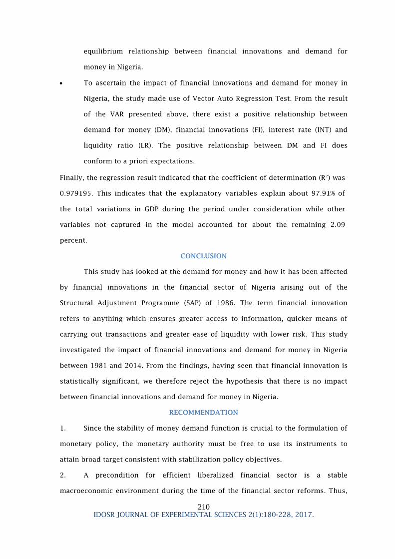
REGRESSION RESULT

UNIT ROOT TESTS

LDM @ LEVEL

Null Hypothesis: LDM has a unit root

Exogenous: Constant, Linear Trend

Lag Length: 0 (Automatic - based on SIC, maxlag=1)

t-Statistic Prob.*

Augmented Dickey-Fuller test statistic -

0.600702

0.9723

Test critical

values:

1% level -

4.262735

5% level -

3.552973

10%

level

-

3.209642

*MacKinnon (1996) one-sided p-values.

Augmented Dickey-Fuller Test Equation

Dependent Variable: D(LDM)

Method: Least Squares

Date: 11/08/16 Time: 01:33



Variable Coeffici

ent

Std. Error t-Statistic Prob.

LDM(-1) -

0.06981

0

0.116214 -

0.600702

0.5525

C 0.44945

3

0.278282 1.615098 0.1168

@TREND(1981) 0.01102

3

0.032480 0.339374 0.7367

R-squared 0.04048

8

Mean dependent

var

0.1795

79

Adjusted R-

squared

-

0.02348

0

S.D. dependent var 0.4460

35

S.E. of regression 0.45124

1

Akaike info

criterion

1.3328

77

Sum squared

resid

6.10855

0

Schwarz criterion 1.4689

23

Log likelihood -

18.9924

7

Hannan-Quinn

criter.

1.3786

52

F-statistic 0.63294

3

Durbin-Watson

stat

1.8806

74

Prob(F-statistic) 0.53797


0

LDM @ 1ST

DIFFERENCE

Null Hypothesis: D(LDM) has a unit root



t-Statistic Prob.*


5.424532

0.0006

Test critical

values:

1% level -

4.273277

5% level -

3.557759

10%

level

-

3.212361



Dependent Variable: D(LDM,2)


Date: 11/08/16 Time: 01:34



Variable Coeffici

ent


D(LDM(-1)) -

1.00214

6

0.184743 -

5.424532

0.0000

C 0.34928

5

0.183176 1.906823 0.0665

@TREND(1981) -

0.00943

5

0.008885 -

1.061888

0.2971

R-squared 0.50418

7

Mean dependent

var

-

0.0031

15

Adjusted R-

squared

0.46999

3


70


6

Akaike info

criterion

1.3688

56

Sum squared

resid

6.10565

4


69

Log likelihood -

18.9017

0

Hannan-Quinn

criter.

1.4144

05

F-statistic 14.7449

0

Durbin-Watson

stat

2.0102

00



8

LFI @ LEVEL

Null Hypothesis: LFI has a unit root



t-Statistic Prob.*


2.216232

0.4655

Test critical

values:

1% level -

4.262735

5% level -

3.552973

10%

level

-

3.209642



Dependent Variable: D(LFI)


Date: 11/08/16 Time: 01:34



Variable Coeffici

ent


LFI(-1) -

0.22478

4

0.101426 -

2.216232

0.0344

C 1.00924

1

0.421651 2.393546 0.0231

@TREND(1981) 0.07888

0

0.034608 2.279209 0.0299

R-squared 0.14777

4

Mean dependent

var

0.2540

80

Adjusted R-

squared

0.09095

9


52


1

Akaike info

criterion

1.5972

10

Sum squared

resid

7.95676

7


57

Log likelihood -

23.3539

7

Hannan-Quinn

criter.

1.6429

86

F-statistic 2.60096 Durbin-Watson 1.8001


6 stat 03


9

LFI @ 1ST

DIFFERENCE

Null Hypothesis: D(LFI) has a unit root



t-Statistic Prob.*


5.294050

0.0008

Test critical

values:

1% level -

4.273277

5% level -

3.557759

10%

level

-

3.212361



Dependent Variable: D(LFI,2)


Date: 11/08/16 Time: 01:35



Variable Coeffici

ent


D(LFI(-1)) -

1.01827

0

0.192342 -

5.294050

0.0000

C 0.24115

1

0.211238 1.141609 0.2630

@TREND(1981) 0.00210

8

0.010826 0.194688 0.8470

R-squared 0.49724

4

Mean dependent

var

-

0.0067

81

Adjusted R-

squared

0.46257

1


35


2

Akaike info

criterion

1.7511

34

Sum squared

resid

8.94856

6


47

Log likelihood -

25.0181

5

Hannan-Quinn

criter.

1.7966

83



2 stat 66


7

INT @ LEVEL

Null Hypothesis: INT has a unit root



t-Statistic Prob.*


2.992615

0.1493

Test critical

values:

1% level -

4.262735

5% level -

3.552973

10%

level

-

3.209642



Dependent Variable: D(INT)


Date: 11/08/16 Time: 01:36



Variable Coeffici

ent


INT(-1) -

0.40220

6

0.134400 -

2.992615

0.0055

C 6.21420

5

2.114246 2.939206 0.0063

@TREND(1981) -

0.04786

2

0.059106 -

0.809770

0.4244

R-squared 0.23964

9

Mean dependent

var

0.1969

70

Adjusted R-

squared

0.18895

9


39


9

Akaike info

criterion

5.2700

49

Sum squared

resid

313.205

9


95

Log likelihood -

83.9558

0

Hannan-Quinn

criter.

5.3158

24



6 stat 04


4

INT @ 1ST

DIFFERENCE

Null Hypothesis: D(INT) has a unit root



t-Statistic Prob.*


6.036610

0.0001

Test critical

values:

1% level -

4.284580

5% level -

3.562882

10%

level

-

3.215267



Dependent Variable: D(INT,2)


Date: 11/08/16 Time: 01:37



Variable Coeffici

ent


D(INT(-1)) -

1.74680

1

0.289368 -

6.036610

0.0000

D(INT(-1),2) 0.35521

0

0.179965 1.973773 0.0587

C 1.58582

5

1.428137 1.110415 0.2766

@TREND(1981) -

0.07341

0

0.070868 -

1.035880

0.3094

R-squared 0.68870

0

Mean dependent

var

0.0161

29

Adjusted R-

squared

0.65411

1


65


3

Akaike info

criterion

5.4438

41

Sum squared

resid

324.370

7


72

Log likelihood -

80.3795

Hannan-Quinn

criter.

5.5041

57


4

F-statistic 19.9110

2

Durbin-Watson

stat

1.9427

59


1

LR @ LEVEL

Null Hypothesis: LR has a unit root



t-Statistic Prob.*


3.179814

0.1058

Test critical

values:

1% level -

4.262735

5% level -

3.552973

10%

level

-

3.209642



Dependent Variable: D(LR)


Date: 11/08/16 Time: 01:37



Variable Coeffici

ent


LR(-1) -

0.49633

2

0.156088 -

3.179814

0.0034

C 24.1866

0

7.989827 3.027175 0.0050

@TREND(1981) -

0.05686

8

0.155012 -

0.366860

0.7163

R-squared 0.25228

2

Mean dependent

var

0.3787

88

Adjusted R-

squared

0.20243

4


82


1

Akaike info

criterion

7.1927

16

Sum squared

resid

2142.07

1


62

Log likelihood -

115.679

Hannan-Quinn

criter.

7.2384

91


8

F-statistic 5.06103

4

Durbin-Watson

stat

1.8337

92


6

LR @ 1ST

DIFFERENCE

Null Hypothesis: D(LR) has a unit root



t-Statistic Prob.*


6.057269

0.0001

Test critical

values:

1% level -

4.273277

5% level -

3.557759

10%

level

-

3.212361



Dependent Variable: D(LR,2)


Date: 11/08/16 Time: 01:38



Variable Coeffici

ent


D(LR(-1)) -

1.11807

1

0.184583 -

6.057269

0.0000

C 0.56748

4

3.740482 0.151714 0.8805

@TREND(1981) -

0.01162

2

0.188964 -

0.061504

0.9514

R-squared 0.55864

6

Mean dependent

var

0.0234

38

Adjusted R-

squared

0.52820

8


93


0

Akaike info

criterion

7.5048

83

Sum squared

resid

2822.11

4


95

Log likelihood -

117.078

Hannan-Quinn

criter.

7.5504

31


1

F-statistic 18.3534

3

Durbin-Watson

stat

1.9956

71


7

JOHANSEN COINTEGRATION ESTIMATE

Date: 11/08/16 Time: 01:39



Trend assumption: Linear deterministic trend

Series: LDM LFI INT LR

Lags interval (in first differences): 1 to 2


Hypothesiz

ed

Trace 0.05

No. of

CE(s)


Value

Prob.**

None 0.497912 40.43526 47.85613 0.2073

At most 1 0.294089 19.07690 29.79707 0.4874

At most 2 0.210651 8.280625 15.49471 0.4359

At most 3 0.030108 0.947695 3.841466 0.3303


* denotes rejection of the hypothesis at the 0.05 level

**MacKinnon-Haug-Michelis (1999) p-values

Unrestricted Cointegration Rank Test (Maximum Eigenvalue)

Hypothesiz

ed

Max-Eigen 0.05

No. of

CE(s)


Value

Prob.**

None 0.497912 21.35837 27.58434 0.2552

At most 1 0.294089 10.79627 21.13162 0.6676

At most 2 0.210651 7.332931 14.26460 0.4505

At most 3 0.030108 0.947695 3.841466 0.3303

Max-eigenvalue test indicates no cointegration at the 0.05 level

* denotes rejection of the hypothesis at the 0.05 level

**MacKinnon-Haug-Michelis (1999) p-values

Unrestricted Cointegrating Coefficients (normalized by

b'*S11*b=I):

LDM LFI INT LR

0.394569 -0.325162 0.261909 0.119260

-2.304251 1.704742 0.155147 -0.018753

-1.708007 1.428216 0.398703 -0.127959

-1.933799 1.905265 0.246283 -0.014673


Unrestricted Adjustment Coefficients (alpha):

D(LDM) 0.238154 0.095901 0.076678 -0.009315

D(LFI) 0.205504 -0.119113 0.036512 -0.055570

D(INT) -1.242553 0.904655 -0.135503 -0.287845

D(LR) -2.733803 -0.587878 3.169971 -0.221545

1 Cointegrating

Equation(s):

Log

likelihood

-209.3323

Normalized cointegrating coefficients (standard error in

parentheses)

LDM LFI INT LR

1.000000 -0.824094 0.663785 0.302255

(0.20197) (0.21362) (0.08197)

Adjustment coefficients (standard error in

parentheses)

D(LDM) 0.093968

(0.02973)

D(LFI) 0.081085

(0.03848)

D(INT) -0.490273

(0.23070)

D(LR) -1.078674

(0.65599)

2 Cointegrating

Equation(s):

Log

likelihood

-203.9342


parentheses)

LDM LFI INT LR

1.000000 0.000000 -6.486035 -2.574006

(1.90087) (0.74976)

0.000000 1.000000 -8.675980 -3.490212

(2.54940) (1.00556)


parentheses)

D(LDM) -0.127013 0.086049

(0.16924) (0.12564)

D(LFI) 0.355553 -0.269880

(0.21974) (0.16312)

D(INT) -2.574826 1.946235

(1.28658) (0.95510)

D(LR) 0.275944 -0.113252

(3.87508) (2.87670)


3 Cointegrating

Equation(s):

Log

likelihood

-200.2677


parentheses)

LDM LFI INT LR

1.000000 0.000000 0.000000 -0.829441

(0.31587)

0.000000 1.000000 0.000000 -1.156611

(0.41157)

0.000000 0.000000 1.000000 0.268973

(0.09775)


parentheses)

D(LDM) -0.257979 0.195561 0.107825

(0.20393) (0.15831) (0.03533)

D(LFI) 0.293189 -0.217732 0.049901

(0.27116) (0.21050) (0.04698)

D(INT) -2.343386 1.752707 -0.239107

(1.59108) (1.23516) (0.27567)

D(LR) -5.138389 4.414152 0.456663

(4.36127) (3.38565) (0.75563)

LAG LENGTH CRITERIA

VAR Lag Order Selection

Criteria

Endogenous variables: LDM LFI INT LR

Exogenous variables: C

Date: 11/08/16 Time: 01:45

Sample: 1981 2014

Included observations: 30

Lag LogL LR FPE AIC SC HQ

0 -296.4460 NA 5874.188 20.02973 20.21656 20.08950

1 -207.4328 148.3554

*

45.75186

*

15.16219

*

16.09632

*

15.46102

*

2 -196.2184 15.70008 67.07943 15.48123 17.16267 16.01913

3 -189.3904 7.738410 146.4182 16.09269 18.52144 16.86967

4 -171.8740 15.18093 190.0998 15.99160 19.16765 17.00764

* indicates lag order selected by the

criterion

LR: sequential modified LR test statistic (each test at 5%

level)

FPE: Final prediction error

AIC: Akaike information

criterion

SC: Schwarz information

criterion

HQ: Hannan-Quinn information criterion


VECTOR AUTO REGRESSION

Vector Autoregression Estimates

Date: 11/08/16 Time: 01:45



Standard errors in ( ) & t-statistics in [ ]

LDM LFI INT LR

LDM(-1) 0.910003 0.329785 0.088475 -3.503918

(0.11367) (0.14418) (0.89490) (2.33294)

[ 8.00539] [ 2.28739] [ 0.09887] [-1.50194]

LFI(-1) 0.055421 0.736309 -0.270452 2.824720

(0.09463) (0.12002) (0.74494) (1.94200)

[ 0.58569] [ 6.13509] [-0.36305] [ 1.45454]

INT(-1) 0.050430 -0.006383 0.578862 0.471902

(0.01985) (0.02518) (0.15631) (0.40747)

[ 2.53997] [-0.25348] [ 3.70341] [ 1.15812]

LR(-1) 0.006295 0.012396 -0.071545 0.432908

(0.00788) (0.01000) (0.06205) (0.16176)

[ 0.79863] [ 1.23995] [-1.15298] [ 2.67617]

C -0.689861 0.065016 10.88040 16.98132

(0.48977) (0.62118) (3.85571) (10.0515)

[-1.40855] [ 0.10466] [ 2.82189] [ 1.68943]

R-squared 0.979195 0.978826 0.451368 0.322656

Adj. R-squared 0.976223 0.975801 0.372992 0.225893

Sum sq. resids 4.686795 7.539412 290.4732 1974.059

S.E. equation 0.409128 0.518907 3.220876 8.396554

F-statistic 329.4577 323.5934 5.759011 3.334485

Log likelihood -14.62095 -22.46498 -82.71253 -114.3321

Akaike AIC 1.189149 1.664544 5.315911 7.232247

Schwarz SC 1.415892 1.891288 5.542655 7.458991

Mean dependent 6.729670 9.579111 13.13455 46.39848

S.D. dependent 2.653256 3.335737 4.067593 9.543343

Determinant resid covariance

(dof adj.)

27.43689

Determinant resid covariance 14.22038

Log likelihood -231.1020

Akaike information criterion 15.21831


SYSTEM EQUATION ESTIMATE

System: UNTITLED

Estimation Method: Least Squares

Date: 11/08/16 Time: 01:47

Sample: 1982 2014



Total system (balanced) observations 132

Coefficie

nt


C(1) 0.910003 0.113674 8.005387 0.0000

C(2) 0.055421 0.094625 0.585686 0.5593

C(3) 0.050430 0.019854 2.539975 0.0125

C(4) 0.006295 0.007882 0.798630 0.4262

C(5) -

0.689861

0.489767 -

1.408549

0.1617

C(6) 0.329785 0.144175 2.287388 0.0241

C(7) 0.736309 0.120016 6.135094 0.0000

C(8) -

0.006383

0.025182 -

0.253481

0.8004

C(9) 0.012396 0.009997 1.239947 0.2176

C(10) 0.065016 0.621184 0.104665 0.9168

C(11) 0.088475 0.894902 0.098865 0.9214

C(12) -

0.270452

0.744943 -

0.363050

0.7173

C(13) 0.578862 0.156305 3.703410 0.0003

C(14) -

0.071545

0.062052 -

1.152983

0.2514

C(15) 10.88040 3.855713 2.821891 0.0057

C(16) -

3.503918

2.332935 -

1.501935

0.1359

C(17) 2.824720 1.942004 1.454538 0.1486

C(18) 0.471902 0.407474 1.158117 0.2493

C(19) 0.432908 0.161764 2.676166 0.0086

C(20) 16.98132 10.05152 1.689427 0.0939

Determinant residual

covariance

14.22038

Equation: LDM = C(1)*LDM(-1) + C(2)*LFI(-1) + C(3)*INT(-1) +

C(4)*LR(-1) +

C(5)

Observations: 33

R-squared 0.979195 Mean dependent

var

6.7296

70

Adjusted R-

squared

0.976223 S.D. dependent var 2.6532

56

S.E. of

regression

0.409128 Sum squared resid 4.6867

95

Durbin-Watson

stat

2.370440

Equation: LFI = C(6)*LDM(-1) + C(7)*LFI(-1) + C(8)*INT(-1) +

C(9)*LR(-1) +

C(10)

Observations: 33


var

9.5791

11


Adjusted R-

squared


37

S.E. of

regression


12

Durbin-Watson

stat

2.085294

Equation: INT = C(11)*LDM(-1) + C(12)*LFI(-1) + C(13)*INT(-1) +

C(14)*LR(

-1) + C(15)

Observations: 33


var

13.134

55

Adjusted R-

squared


93

S.E. of

regression


31

Durbin-Watson

stat

2.169167

Equation: LR = C(16)*LDM(-1) + C(17)*LFI(-1) + C(18)*INT(-1) +

C(19)*LR(

-1) + C(20)

Observations: 33


var

46.398

48

Adjusted R-

squared


43

S.E. of

regression


59

Durbin-Watson

stat

1.778772

LM TEST OF SERIAL CORRELATION

VAR Residual Serial Correlation

LM Tests

Null Hypothesis: no serial

correlation at lag order h

Date: 11/08/16 Time: 01:48

Sample: 1981 2014


Lags LM-Stat Prob

1 15.11452 0.5163

Probs from chi-square with 16

df.

©idosr publications international digital organization for … · ©idosr publications...

Documents