ideal spatial adaptation b - stanford universitystatweb.stanford.edu/~imj/weblist/1994/isaws.pdf ·...
TRANSCRIPT
Ideal Spatial Adaptation by Wavelet Shrinkage
David L. Donoho
Iain M. Johnstone
Department of Statistics, Stanford University, Stanford, CA, 94305-4065, U.S.A.
June 1992
Revised April 1993
Abstract
With ideal spatial adaptation, an oracle furnishes information about how best to
adapt a spatially variable estimator, whether piecewise constant, piecewise polynomial,
variable knot spline, or variable bandwidth kernel, to the unknown function. Estimation
with the aid of an oracle o�ers dramatic advantages over traditional linear estimation
by nonadaptive kernels; however, it is a priori unclear whether such performance can
be obtained by a procedure relying on the data alone. We describe a new principle for
spatially-adaptive estimation: selective wavelet reconstruction. We show that variable-
knot spline �ts and piecewise-polynomial �ts, when equipped with an oracle to select the
knots, are not dramatically more powerful than selective wavelet reconstruction with
an oracle. We develop a practical spatially adaptive method, RiskShrink, which works
by shrinkage of empirical wavelet coe�cients. RiskShrink mimics the performance of
an oracle for selective wavelet reconstruction as well as it is possible to do so. A new
inequality in multivariate normal decision theory which we call the oracle inequality
shows that attained performance di�ers from ideal performance by at most a factor
� 2 logn, where n is the sample size. Moreover no estimator can give a better guarantee
than this. Within the class of spatially adaptive procedures, RiskShrink is essentially
optimal. Relying only on the data, it comes within a factor log2n of the performance
of piecewise polynomial and variable-knot spline methods equipped with an oracle.
In contrast, it is unknown how or if piecewise polynomial methods could be made to
function this well when denied access to an oracle and forced to rely on data alone.
Keywords: Minimax estimation subject to doing well at a point; Orthogonal Wavelet
Bases of Compact Support; Piecewise-Polynomial �tting; Variable-Knot Spline.
1
1 Introduction
Suppose we are given data
yi = f(ti) + ei; i = 1; : : : ; n; (1)
ti = i=n, where ei are independently distributed as N(0; �2), and f(�) is an unknown
function which we would like to recover. We measure performance of an estimate f̂(�) in
terms of quadratic loss at the sample points. In detail, let f = (f(ti))ni=1 and f̂ = (f̂(ti))
ni=1
denote the vectors of true and estimated sample values, respectively. Let kvk22;n =Pn
i=1 v2i
denote the usual squared `2n norm; we measure performance by the risk
R(f̂ ; f) = n�1Ekf̂ � fk
22;n;
which we would like to make as small as possible. Although the notation f suggests a
function of a real variable t, in this paper we work only with the equally spaced sample
points ti:
1.1 Spatially Adaptive Methods
We are particularly interested in a variety of spatially adaptive methods which have been
proposed in the statistical literature, such as CART (Breiman, Friedman, Olshen and Stone,
1983), Turbo (Friedman and Silverman, 1989), MARS (Friedman, 1991), and variable-
bandwidth kernel methods (M�uller and Stadtmuller, 1987).
Such methods have presumably been introduced because they were expected to do a
better job in recovery of the functions actually occurring with real data than do traditional
methods based on a �xed spatial scale, such as Fourier series methods, �xed-bandwidth
kernel methods, and linear spline smoothers. Informal conversations with Leo Breiman and
Jerome Friedman have con�rmed this assumption.
We now describe a simple framework which encompasses the most important spatially
adaptive methods, and allows us to develop our main theme e�ciently. We consider esti-
mates f̂ de�ned as
f̂(�) = T (y; d(y))(�) (2)
where T (y; �) is a reconstruction formula with \spatial smoothing" parameter �, and d(y)
is a data-adaptive choice of the spatial smoothing parameter �. A clearer picture of what
we intend emerges from �ve examples.
[1]. Piecewise Constant Reconstruction TPC(y; �). Here � is a �nite list of, say, L real
numbers de�ning a partition (I1; : : : ; IL) of [0; 1] via I1 = [0; �1); I2 = [�1; �1+ �2); : : : ; IL =
[�1+� � �+�L�1; �1+� � �+�L] ,so thatPL
1 �i = 1. Note that L is a variable. The reconstruction
formula is
TPC(y; �)(t) =LX`=1
Ave(yi : ti 2 I`)1I`(t);
piecewise constant reconstruction using the mean of the data within each piece to estimate
the pieces.
[2]. Piecewise Polynomials TPP (D)(y; �). Here the interpretation of � is the same as in
[1], only the reconstruction uses polynomials of degree D.
TPP (D)(y; �)(t) =LX`=1
p̂`(t)1I`(t);
2
where p̂`(t) =PD
k=0 aktk is determined by applying the least squares principle to the data
arising for interval I` Xti2I`
(p̂`(ti)� yi)2 = min!
[3]. Variable-Knot Splines Tspl;D(y; �). Here � de�nes a partition as above, and on each
interval of the partition the reconstruction formula is a polynomial of degree D, but now
the reconstruction must be continuous and have continuous derivatives through order D�1.
In detail, let �` be the left endpoint of I`, ` = 1; : : : ; L. The reconstruction is chosen from
among those piecewise polynomials s(t) satisfying d
dt
k
s
!(�`�) =
d
dt
k
s
!(�`+)
for k = 0; : : : ; D� 1, ` = 2; : : : ; L; subject to this constraint, one solves
nXi=1
(s(ti)� yi)2 = min!
[4]. Variable Bandwidth Kernel Methods TVK;2(y; �). Now � is a function on [0; 1]; �(t)
represents the \bandwidth of the kernel at t"; the smoothing kernel K is a C2 function of
compact support which is also a probability density, and if f̂ = TVK;2(y; �) then
f̂(t) =1
n
nXi=1
yiK
�t � ti
�(t)
���(t): (3)
More re�ned versions of this formula would adjust K for boundary e�ects near t = 0 and
t = 1.
[5]. Variable-Bandwidth High-Order Kernels TVK;D(y; �), D > 2. Here � is again the
local bandwidth, and the reconstruction formula is as in (3), only K(�) is a CD function
integrating to 1, with vanishing intermediate momentsZtjK(t) dt = 0; j = 1; : : : ; D� 1:
As D > 2, K(�) cannot be nonnegative.
These reconstruction techniques, when equipped with appropriate selectors of the spatial
smoothing parameter �, duplicate essential features of certain well-known methods.
[1] The piecewise constant reconstruction formula TPC , equipped with choice of partition
� by recursive partitioning and cross-validatory choice of \pruning constant" as de-
scribed by Breiman, Friedman, Olshen and Stone (1983) results in the method CART
applied to 1-dimensional data.
[2] The spline reconstruction formula Tspl;D, equipped with a backwards deletion scheme
models the methods of Friedman and Silverman (1989) and Friedman (1991) applied
to 1-dimensional data.
[3] The kernel method TK;2 equipped with the variable bandwidth selector described
in Brockmann, Gasser and Herrmann (1992) results in the \Heidelberg" variable
bandwidth smoothing method. Compare also Terrell and Scott (1992).
3
These schemes are computationally feasible and intuitively appealing. However, very
little is known about the theoretical performance of these adaptive schemes, at the level of
uniformity in f and N that we would like.
1.2 Ideal Adaptation with Oracles
To avoid messy questions, we abandon the study of speci�c �-selectors and instead study
ideal adaptation.
For us, ideal adaptation is the performance which can be achieved from smoothing with
the aid of an oracle. Such an oracle will not tell us f , but will tell us, for our method T (y; �),
the \best" choice of � for the true underlying f . The oracle's response is conceptually a
selection �(f) which satis�es
R(T (y;�(f)); f) = Rn;�(T; f)
where Rn;� denotes the ideal risk
Rn;�(T; f) = inf�R(T (y; �); f):
As R measures performance with a selection �(f) based on full knowledge of f rather
than a data-dependent selection d(y), it represents an ideal we cannot expect to attain.
Nevertheless it is the target we shall consider.
Ideal adaptation o�ers, in principle, considerable advantages over traditional nonadap-
tive linear smoothers. Consider the case of a function f which is a piecewise polynomial of
degree D, with a �nite number of pieces I1; : : : ; IL, say:
f =LX`=1
p`(t)1I`(t): (4)
Assume that f has discontinuities at some of the break-points �2; : : : ; �L.
The risk of ideally adaptive piecewise polynomial �ts is essentially �2L(D+1)=n. Indeed,
an oracle could supply the information that one should use I1; : : : ; IL rather than some other
partition. Traditional least-squares theory says that, for data from the traditional linear
model Y = X� + E, with noise Ei independently distributed as N(0; �2), the traditional
least-squares estimator �̂ satis�es
EkX��X�̂k22 = (number of parameters in �)(variance of noise)
Applying this to our setting, �tting a function of the form (4) requires �tting (# pieces)(degree+
1) parameters, so for the risk R(f̂ ; f) = n�1Ekf̂�fk
22;n we get L(D+1)�2=n as advertised.
On the other hand, the risk of a spatially-non-adaptive procedure is far worse. Con-
sider kernel smoothing. Because f has discontinuities, no kernel smoother with �xed non-
spatially varying bandwidth attains a risk R(f̂ ; f) tending to zero faster than Cn�1=2,
C = C(f; kernel). The same result holds for estimates in orthogonal series of polynomials
or sinusoids, for smoothing splines with knots at the sample points and for least squares
smoothing splines with knots equispaced.
Most strikingly, even for piecewise polynomial �ts with equal-width pieces, we have that
R(f̂ ; f) is of size � n�1=2 unless the breakpoints of f form a subset of the breakpoints of
f̂ . But this can happen only for very special n, so in any event
lim supN!1
R(f̂ ; f)n1=2 � C > 0:
4
In short, oracles o�er an improvement|ideally|from risk of order n�1=2 to order n�1. No
better performance than this can be expected, since n�1 is the usual \parametric rate" for
estimating �nite-dimensional parameters.
Can we approach this ideal performance with estimators using the data alone?
1.3 Selective Wavelet Reconstruction as a Spatially Adaptive Method
A new principle for spatially adaptive estimation can be based on recently developed
\wavelets" ideas. Introductions, historical accounts and references to much recent work
may be found in the books by Daubechies (1992), Meyer (1990), Chui (1992) and Frazier,
Jawerth and Weiss (1991). Orthonormal bases of compactly supported wavelets provide a
powerful complement to traditional Fourier methods: they permit an analysis of a signal or
image into localised oscillating components. In a statistical regression context, this spatially
varying decomposition can be used to build algorithms that adapt their e�ective \window
width" to the amount of local oscillation in the data. Since the decomposition is in terms
of an orthogonal basis, analytic study in closed form is possible.
For the purposes of this paper, we discuss a �nite, discrete, wavelet transform. This
transform, along with a careful treatment of boundary correction, has been described by
Cohen, Daubechies, Jawerth, and Vial (1993), with related work in Meyer (1991) and
Malgouyres (1991). To focus attention on our main themes, we employ a simpler periodised
version of the �nite discrete wavelet transform in the main exposition. This version yields
an exactly orthogonal transformation between data and wavelet coe�cient domains. Brief
comments on the minor changes needed for the boundary corrected version are made in
Section 4.6.
Suppose we have data y = (yi)ni=1, with n = 2J+1. For various combinations of pa-
rameters M (number of vanishing moments), S (support width), and j0 (Low-resolution
cuto�), one may construct an n-by-n orthogonal matrix W|the �nite wavelet transform
matrix. Actually there are many such matrices, depending on special �lters: in addition to
the original Daubechies wavelets there are the Coi ets and Symmlets of Daubechies (1993).
For the �gures in this paper we use the Symmlet with parameter N = 8. This has M = 7
vanishing moments and support length S = 15.
This matrix yields a vector w of the wavelet coe�cients of y via|
w =Wy;
and because the matrix is orthogonal we have the inversion formula y =WTw.
The vector w has n = 2J+1 elements. It is convenient to index dyadically n�1 = 2J+1�1
of the elements following the scheme
wj;k : j = 0; : : : ; J ; k = 0; : : : ; 2j � 1;
and the remaining element we label w�1;0. To interpret these coe�cients let Wjk denote
the (j; k)-th row of W . The inversion formula y =WTw becomes
yi =Xj;k
wj;kWjk(i);
expressing y as a sum of basis elementsWjk with coe�cients wj;k. We call theWjk wavelets.
5
The vector Wjk, plotted as a function of i, looks like a localized wiggle, hence the name
\wavelet". For j and k bounded away from extreme cases by the conditions
j0 � j < J � j1; S < k < 2j � S;
we have the approximation
n1=2Wjk(i) � 2j=2 (2jt � k) t = i=n
where is a �xed \wavelet" in the sense of the usual wavelet transform on IR (Meyer, 1990),
Daubechies (1988). This approximation improves with increasing n and increasing j1. Here
is an oscillating function of compact support, usually called the mother wavelet. We
therefore speak of Wjk as being localized to spatial positions near t = k2�j and frequencies
near 2j .
The wavelet can have a smooth visual appearance, if the parameters M and S are
chosen su�ciently large, and favorable choices of so-called quadrature mirror �lters are made
in the construction of the matrixW . Daubechies (1988) described a particular construction
with S = 2M + 1 for which the smoothness (number of derivatives) of is proportional to
M .
For our purposes, the only details we need are
[W1] Wjk has vanishing moments through order M , as long as j � j0:
n�1Xi=0
i`Wjk(i) = 0 ` = 0; : : : ;M; j � j0; k = 0; : : : ; 2j � 1:
[W2] Wjk is supported in [2J�j(k � S); 2J�j(k + S)], provided j � j0.
Because of the spatial localization of wavelet bases, the wavelet coe�cients allow one to
easily answer the question \is there a signi�cant change in the function near t?" by looking
at the wavelet coe�cients at levels j = j0; : : : ; J at spatial indices k with k2�j � t. If these
coe�cients are large, the answer is \yes."
Figures 1 displays four functions { Bumps, Blocks, HeaviSine and Doppler { which
have been chosen because they caricature spatially variable functions arising in imaging,
spectroscopy and other scienti�c signal processing. For all �gures in this article, n = 2048.
Figure 2 depicts the wavelet transforms of the four functions. The large coe�cients occur
exclusively near the areas of major spatial activity. This property suggests that a spatially
adaptive algorithm could be based on the principle of selective wavelet reconstruction. Given
a �nite list � of (j; k) pairs, de�ne TSW (y; �) by
TSW (y; �) = f̂ =X
(j;k)2�
wj;kWjk : (5)
This provides reconstructions by selecting only a subset of the empirical wavelet coe�cients.
Our motivation in proposing this principle is twofold. First, for a spatially inhomo-
geneous function, \most of the action" is concentrated in a small subset of (j; k)-space.
Second, under the noise model underlying (1), noise contaminates all wavelet coe�cients
equally. Indeed, the noise vector e = (ei) is assumed to be a white noise; so its orthogonal
transform z =We is also a white noise. Consequently, the empirical wavelet coe�cient
wj;k = �j;k + zj;k
6
where � =Wf is the wavelet transform of the noiseless data f = (f(ti))n�1i=0 .
Every empirical wavelet coe�cient therefore contributes noise of variance �2, but only
a very few wavelet coe�cients contribute signal. This is the heuristic of our method.
Ideal spatial adaptation can be de�ned for selective wavelet reconstruction in the obvious
way. For the risk measure (1) the ideal risk is
Rn;�(SW; f) = inf�Rn;�(TSW (y; �); f)
with optimal spatial parameter �(f) a list of (j; k) indices attaining
Rn;�(TSW (y;�(f)); f) = Rn;�(SW; f):
Figures 3-6 depict the results of ideal wavelet adaptation for the 4 functions displayed
in Figure 2. Figure 3 shows noisy versions of the four functions of interest; the signal-
to-noise ratio ksignalk2;n=knoisek2;nis 7. Figure 4 shows the noisy data in the wavelet
domain. Figure 5 shows the reconstruction by selective wavelet reconstruction using an
oracle; Figure 6 shows the situation in the wavelet domain. Because the oracle helps us to
select the important wavelet coe�cients, the reconstructions are of high quality.
The theoretical bene�ts of ideal wavelet selection can again be seen in the case (4) where
f is a piecewise polynomial of degree D. Suppose we use a wavelet basis with parameter
M � D. Then properties [W1] and [W2] imply that the wavelet coe�cients �j;k of f all
vanish except for
(i) coe�cients at the coarse levels 0 � j < j0
(ii) coe�cients at j0 � j � J whose associated interval [2�j(k � S); 2�j(k + S)] contains
a breakpoint of f .
There are a �xed number 2j0 of coe�cients satisfying (i), and, in each resolution level
j, (�j;k ; k = 0; : : : ; 2j � 1) at most (# breakpoints)(2S + 1) satisfying (ii). Consequently,
with L denoting again the number of pieces in (4), we have
#f(j; k) : �j;k 6= 0g � 2j0 + (J + 1� j0)(2S + 1)L:
Let �� = f(j; k) : �j;k 6= 0g. Then, because of the orthogonality of the (Wjk),P(j;k)2�� wj;kWjk is the least-squares estimate of f and
R(T (y; ��); f) = n�1#(��)�2
� (C1 + C2J)L�2=n for all n = 2J+1 (6)
with certain constants C1, C2, depending linearly on S, but not on f . Hence
Rn;�(SW; f) = O
�2 logn
n
!: (7)
for every piecewise polynomial of degree D � M . This is nearly as good as the bound
�2L(D+1)n�1 of ideal piecewise polynomial adaptation, and considerably better than the
rate n�1=2 of usual nonadaptive linear methods.
7
1.4 Near-Ideal Spatial Adaptation by Wavelets
Of course, calculations of ideal risk which point to the bene�t of ideal spatial adaptation
prompt the question: How nearly can one approach ideal performance when no oracle is
available and we must rely on data only, and no side information about f?
The bene�t of the wavelet framework is that we can answer such questions precisely. In
Section 2 of this paper we develop new inequalities in multivariate decision theory which
furnish an estimate f̂� which, when presented with data y and knowledge of the noise level
�2, obeys
Rn;�(f̂�; f) � (2 logn + 1)fRn;�(SW; f)+
�2
ng (8)
for every f , every n = 2J+1, and every �.
Thus, in complete generality, it is possible to come within a 2 logn factor of the per-
formance of ideal wavelet adaptation. In small samples n, the factor (2 logn + 1) can be
replaced by a constant which is much smaller: e.g., 5 will do if n � 256; 10 will do if
n � 16384. On the other hand, no radically better performance is possible: to get an
inequality valid for all f , all �, and all n, we cannot even change the constant 2 to 2 � �
and still have (8) hold, neither by f̂� nor by any other measurable estimator sequence.
To illustrate the implications, Figures 7 and 8 show the situation for the four basic
examples, with an estimator ~f�n which has been implemented on the computer, as described
in section 2.3 below. The result, while slightly noisier than the ideal estimate, is still of
good quality { and requires no oracle.
The theoretical properties are also interesting. Our method has the property that for
every piecewise polynomial (4) of degree D �M with � L pieces,
Rn;�(f̂�; f) � (C1 + C2 logn)(2 logn + 1)L�2=n;
where C1 and C2 are as in (6); this result is merely a combination of (7) and (8). Hence
in this special case we have an actual estimator coming within C log2 n of ideal piecewise
polynomial �ts.
1.5 Universality of Wavelets as a Spatially Adaptive Procedure
This last calculation is not essentially limited to piecewise polynomials; something like it
holds for all f . In section 3 we show that, for constants Ci not depending on f , n, or �,
Rn;�(SW; f) � (C1 + C2J)Rn;�(PP (D); f)
for every f , every n = 2J+1 and every � > 0.
We interpret this result as saying that selective wavelet reconstruction is essentially
as powerful as variable-partition piecewise constant �ts, variable-knot least-squares splines,
or piecewise polynomial �ts. Suppose that the function f is such that, furnished with an
oracle, piecewise polynomials, piecewise constants, or variable-knot splines would improve
the rate of convergence over traditional �xed-bandwidth kernel methods, say from rate of
convergence n�r1 (with �xed-bandwidth) to n�r2 , r2 > r1. Then, furnished with an oracle,
selective wavelet adaptation o�ers an improvement to log2 nn�r2 ; this is essentially the
same bene�t at the level of rates.
We know of no proof that existing procedures for �tting piecewise polynomials and
variable-knot splines, such as those current in the statistical literature, can attain anything
like the performance of ideal methods.
8
In contrast, for selective wavelet reconstruction, it is easy to o�er performance compa-
rable to that with an oracle, using the estimator f̂�. And wavelet selection with an oracle
o�ers the advantages of other spatially-variable methods.
The main assertion of this paper is therefore that, from this (theoretical) perspective,
it is cleaner and more elegant to abandon the ideal of �tting piecewise polynomials with
optimal partitions, and turn instead to RiskShrink, about which we have theoretical results,
and an order O(n) algorithm.
1.6 Contents
Section 2 discusses the problem of mimicking ideal wavelet selection; Section 3 shows why
wavelet selection o�ers the same advantages as piecewise polynomial �ts; Section 4 dis-
cusses variations and relations to other work. Section 5 contains certain proofs. Related
manuscripts by the authors, currently under publication review and available as LaTeX
�les by anonymous ftp from playfair.stanford.edu, are cited in the text by [�lename.tex].
2 Decision Theory and Spatial Adaptation
In this section we solve a new problem in multivariate normal decision theory and apply it
to function estimation.
2.1 Oracles for Diagonal Linear Projection
Consider the following problem from multivariate normal decision theory. We are given
observations w = (wi)ni=1 according to
wi = �i + �zi i = 1; : : : ; n (9)
where zi are independent and identically distributed as N(0; 1), � > 0 is the (known) noise
level, and � = (�i) is the object of interest. We wish to estimate with `2-loss and so de�ne
the risk measure
R(�̂; �) = Ek�̂� �k22;n: (10)
We consider a family of diagonal linear projections:
TDP (w; �) = (�iwi)ni=1; �i 2 f0; 1g:
Such estimators \keep" or \kill" each coordinate. Suppose we had available an or-
acle which would supply for us the coe�cients �DP (�) optimal for use in the diagonal
projection scheme. These ideal coe�cients are �i = 1fj�ij>�g meaning that ideal diagonal
projection consists in estimating only those �i larger than the noise level. Supplied with
such coe�cients, we would attain the ideal risk
R�(DP; �) =nXi=1
�T (j�ij; �)
with �T (�; �) = min(�2; �2).
In general the ideal risk R�(DP; �) cannot be attained for all � by any estimator, linear
or nonlinear. However surprisingly simple estimates do come remarkably close.
9
Motivated by the idea that only very few wavelet coe�cients contribute signal, we
consider threshold rules, that retain only observed data that exceeds a multiple of the noise
level. De�ne `hard' and `soft' threshold non-linearities by
�H(w; �) = wIfjwj> �g (11)
�S(w; �) = sgn(w)(jwj � �)+: (12)
The hard threshold rule is reminiscent of subset selection rules used in model selection and
we return to it later. For now, we focus on soft thresholding.
Theorem 1 Assume model (9){(10). The estimator
�̂ui = �S(wi; �(2 logn)
1=2) i = 1; : : : ; n
satis�es
Ek�̂u� �k
22;n � (2 logn+ 1)f�2 +
nXi=1
min(�2i ; �2)g for all � 2 IRn
: (13)
In \Oracular" notation, we have
R(�̂�; �) � (2 logn+ 1)(�2 +R�(DP; �)): � 2 IRn
Now �2 denotes the mean-squared loss for estimating one parameter unbiasedly, so the
inequality says that we can mimick the performance of an oracle plus one extra parameter
to within a factor of essentially 2 logn.
A short proof appears in the Appendix. However it is natural and more revealing to
look for `optimal' thresholds ��n which yield the smallest possible constant ��n in place of
2 logn+1 among soft threshold estimators. We give the result here and outline the approach
in Section 2.4.
Theorem 2 Assume model (9){(10). The minimax threshold ��n de�ned at (20) and solv-
ing (22) below yields an estimator
�̂�
i = �S(wi; ��
n�) i = 1; : : : ; n (14)
which satis�es
Ek�̂�� �k
22;n � ��nf�
2 +nXi=1
min(�2i ; �2)g for all � 2 IRn
: (15)
The coe�cient ��n, de�ned at (19), satis�es ��n � 2 logn + 1, and the threshold ��
n �
(2 logn)1=2. Asymptotically
��n � 2 logn; ��
n � (2 logn)1=2; n!1:
Table 1 shows that this constant ��n is much smaller than 2 logn + 1 when n is on the
order of a few hundred. For n = 256, we get ��n � 4:44. For large n, however, the � 2 logn
upper bound is sharp. This holds even if we extend from soft co-ordinatewise thresholds to
allow completely arbitrary estimator sequences into contention.
10
Theorem 3
inf�̂
sup�2IRn
Ek�̂ � �k22;n
�2 +Pn
1 min(�2i ; �
2)� 2 logn as n!1: (16)
Hence an inequality of the form (13) or (15) cannot be valid for any estimator sequence
with (2 � � + o(1)) logn in place of ��n. In this sense, an oracle for diagonal projection
cannot be mimicked essentially more faithfully than by �̂�.
The use of soft thresholding rules (12) was suggested to us in prior work on multivariate
normal decision theory by Bickel (1983) and ourselves [mrlp.tex]. However it is worth men-
tioning that a more traditional hard threshold estimator (11) exhibits the same asymptotic
performance.
Theorem 4 With (`n) a thresholding sequence su�ciently close to (2 logn)1=2, the hard
threshold estimator
�̂+i = wi1fjwij>`n�g
satis�es, for an Ln � 2 logn, the inequality
R(�̂+; �) � Lnf�2 +
nXi=1
min(�2i ; �2)g for all � 2 IRn
:
Here, su�ciently close to (2 logn)1=2 means (1 � ) log logn � `2n � 2 logn � o(logn) for
some > 0.
2.2 Adaptive Wavelet Shrinkage
We now apply the preceding results to function estimation. Let n = 2J+1, and letW denote
the wavelet transform mentioned in section 1.3. W is an orthogonal transformation of IRn
into IRn. In particular, if f = (fi) and f̂ = (f̂i) are two n-vectors and (�j;k) and (�̂j;k) their
W transforms, we have the Parseval relation
kf � f̂k2;n = k� � �̂k2;n (17)
Now let (yi) be data as in model (1) and let w =Wy be the discrete wavelet transform.
Then with � = �
wj;k = �j;k + �zj;k j = 0; : : : ; J ; k = 0; : : : ; 2j � 1:
As in the introduction, we de�ne selective wavelet reconstruction via TSW (y; �), c.f. (5),
and observe that
TSW =WT� TDP �W (18)
in the sense that (5) is realized by wavelet transform, followed by diagonal linear projection
or shrinkage, followed by inverse wavelet transform. Because of the Parseval relation (17),
we have
EkTSW (y; �)� fk22;n = EkTDP (w; �)� �k22;n:
Also if �̂� denotes the nonlinear estimator (14) and
f̂�� W
T� �̂
��W
then again by Parseval Ekf̂� � fk22;n = Ek�̂
�� �k
22;n, and we conclude immediately:
11
Corollary 1 For all f and all n = 2J+1,
R(f̂�; f) � ��nf�2
n+Rn;�(SW; f)g:
Moreover, no estimator can satisfy a better inequality than this for all f and all n, in the
sense that for no measurable estimator can such an inequality hold, for all n and f , with
��n replaced by (2 � � + o(1)) logn. The same type of inequality holds for an estimator
f̂+ =W
T� �̂
+�W derived from hard thresholding, with Ln in place of ��n.
Hence, we have achieved, by very simple means, essentially the best spatial adaptation
possible via wavelets.
2.3 Implementation
We have developed a computer software package which runs in the numerical computing
environment Matlab. In addition, an implementation by G.P. Nason in the S language is
available by anonymous ftp from Statlib at lib.stat.cmu.edu ; other implementations are
also in development. They implement the following modi�cation of f̂�.
De�nition 1 Let ~�� denote the estimator in the wavelet domain obtained by
~��j;k =
(wj;k j < j0
�S(wj;k; ��
n�) j0 � j � J:
RiskShrink is the estimator~f�n � W
T� ~�� �W
The name RiskShrink for the estimator emphasises that shrinkage of wavelet coe�cients
is performed by soft thresholding, and that a mean squared error , or \risk" approach has
been taken to specify the threshold. Alternative choices of threshold lead to the estima-
tors VisuShrink introduced in Section 4.2 below, and SureShrink discussed in our report
[ausws.tex].
The rationale behind this rule is as follows. The wavelets Wj;k at levels j < j0 do
not have vanishing means, and so the corresponding coe�cients �j;k should not generally
cluster around zero. Hence, those coe�cients (a �xed number, independent of n) should
not be shrunken towards zero. Let gSW denote the selective wavelet reconstruction where
the levels below j0 are never shrunk. We have, evidently, the risk bound
R( ~f�; f) � ��nf�2
n+Rn;�(gSW; f)g
and of course Rn;�(gSW; f) � 2j0�2=n+Rn;�(SW; f), so RiskShrink is never dramatically
worse than f̂�; it is typically much better on functions having non-zero average values.
Figure 7 shows the reconstructions of the four test functions; Figure 8 shows the sit-
uation in the wavelet domains. Evidently the methods do a good job of adapting to the
spatial variability of functions.
The reader will note that occasionally these reconstructions exhibit �ne scale noise
artifacts. This is to some extent inevitable: no hypothesis of smoothness of the underlying
function is being made.
12
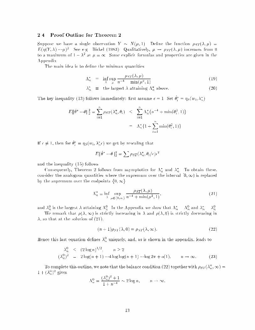
2.4 Proof Outline for Theorem 2
Suppose we have a single observation Y � N(�; 1). De�ne the function �ST (�; �) =
E(�(Y; �)� �)2. See e.g. Bickel (1983). Qualitatively, � ! �ST (�; �) increases from 0
to a maximum of 1 + �2 at � =1. Some explicit formulas and properties are given in the
Appendix.
The main idea is to de�ne the minimax quantities
��n � inf�sup�
�ST (�; �)
n�1 +min(�2; 1)(19)
��
n � the largest � attaining ��n above: (20)
The key inequality (13) follows immediately: �rst assume � = 1. Set �̂�i = �S(wi; ��
n).
Ek�̂�� �k
22 =
nXi=1
�ST (��
n; �i) �
nXi=1
��nfn�1 +min(�2i ; 1)g
= ��nf1 +nXi=1
min(�2i ; 1)g
If � 6= 1, then for �̂�i = �S(wi; ��
n�) we get by rescaling that
Ek�̂�� �k
22 =
X�ST (�
�
n; �i=�)�2
and the inequality (15) follows.
Consequently, Theorem 2 follows from asymptotics for ��n and ��
n. To obtain these,
consider the analogous quantities where the supremum over the interval [0;1) is replaced
by the supremum over the endpoints f0;1g.
�0n � inf
�sup
�2f0;1g
�ST (�; �)
n�1 +min(�2; 1); (21)
and �0n is the largest � attaining �0n. In the Appendix we show that ��n = �0
n and ��
n = �0n.
We remark that �(�;1) is strictly increasing in � and �(�; 0) is strictly decreasing in
�, so that at the solution of (21),
(n+ 1)�ST (�; 0) = �ST (�;1): (22)
Hence this last equation de�nes �0n uniquely, and, as is shown in the appendix, leads to
�0n � (2 logn)1=2; n � 2
(�0n)2 = 2 log(n+ 1)� 4 log log(n+ 1)� log 2� + o(1); n!1: (23)
To complete this outline, we note that the balance condition (22) together with �ST (�0n;1) =
1 + (�0n)2 gives
�0n =
(�0n)2 + 1
1 + n�1� 2 logn; n!1:
13
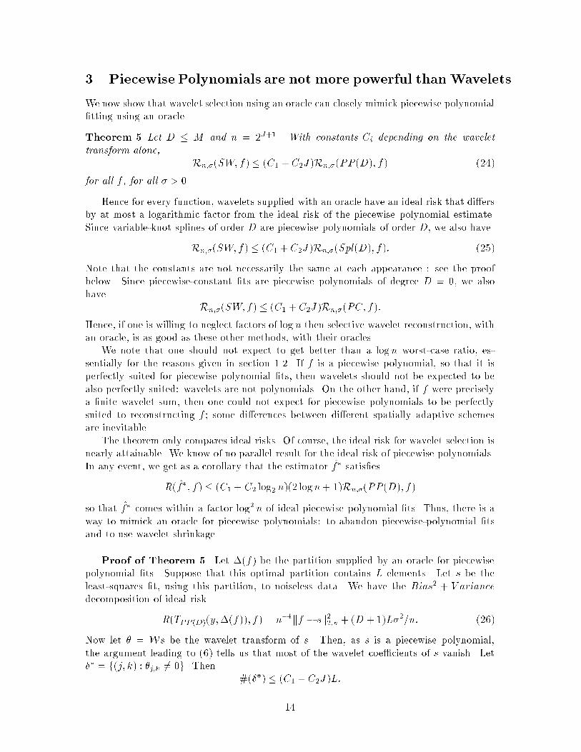
3 Piecewise Polynomials are not more powerful than Wavelets
We now show that wavelet selection using an oracle can closely mimick piecewise polynomial
�tting using an oracle.
Theorem 5 Let D � M and n = 2J+1. With constants Ci depending on the wavelet
transform alone,
Rn;�(SW; f) � (C1 + C2J)Rn;�(PP (D); f) (24)
for all f , for all � > 0.
Hence for every function, wavelets supplied with an oracle have an ideal risk that di�ers
by at most a logarithmic factor from the ideal risk of the piecewise polynomial estimate.
Since variable-knot splines of order D are piecewise polynomials of order D, we also have
Rn;�(SW; f) � (C1 + C2J)Rn;�(Spl(D); f): (25)
Note that the constants are not necessarily the same at each appearance : see the proof
below. Since piecewise-constant �ts are piecewise polynomials of degree D = 0, we also
have
Rn;�(SW; f) � (C1 + C2J)Rn;�(PC; f):
Hence, if one is willing to neglect factors of log n then selective wavelet reconstruction, with
an oracle, is as good as these other methods, with their oracles.
We note that one should not expect to get better than a logn worst-case ratio, es-
sentially for the reasons given in section 1.2. If f is a piecewise polynomial, so that it is
perfectly suited for piecewise polynomial �ts, then wavelets should not be expected to be
also perfectly suited: wavelets are not polynomials. On the other hand, if f were precisely
a �nite wavelet sum, then one could not expect for piecewise polynomials to be perfectly
suited to reconstructing f ; some di�erences between di�erent spatially adaptive schemes
are inevitable.
The theorem only compares ideal risks. Of course, the ideal risk for wavelet selection is
nearly attainable. We know of no parallel result for the ideal risk of piecewise polynomials.
In any event, we get as a corollary that the estimator f̂� satis�es
R(f̂�; f) � (C1 + C2 log2 n)(2 logn+ 1)Rn;�(PP (D); f)
so that f̂� comes within a factor log2 n of ideal piecewise polynomial �ts. Thus, there is a
way to mimick an oracle for piecewise polynomials: to abandon piecewise-polynomial �ts
and to use wavelet shrinkage.
Proof of Theorem 5. Let �(f) be the partition supplied by an oracle for piecewise
polynomial �ts. Suppose that this optimal partition contains L elements. Let s be the
least-squares �t, using this partition, to noiseless data. We have the Bias2 + V ariance
decomposition of ideal risk
R(TPP (D)(y;�(f)); f) = n�1kf � sk
22;n + (D + 1)L�2=n: (26)
Now let � = Ws be the wavelet transform of s. Then, as s is a piecewise polynomial,
the argument leading to (6) tells us that most of the wavelet coe�cients of s vanish. Let
�� = f(j; k) : �j;k 6= 0g. Then
#(��) � (C1 + C2J)L:
14
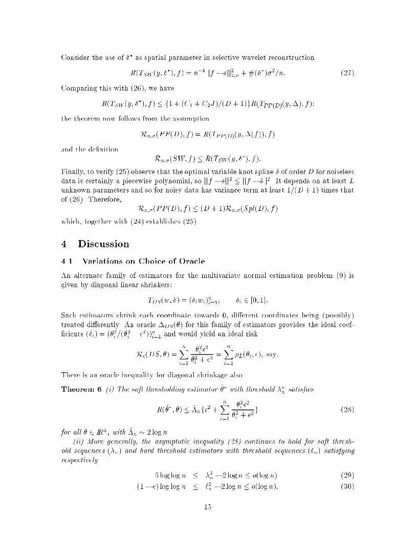
Consider the use of �� as spatial parameter in selective wavelet reconstruction.
R(TSW (y; ��); f) = n�1jjf � sjj
22;n +#(��)�2=n: (27)
Comparing this with (26), we have
R(TSW (y; ��); f) � f1 + (C1 + C2J)=(D+ 1)gR(TPP (D)(y;�); f);
the theorem now follows from the assumption
Rn;�(PP (D); f) = R(TPP (D)(y;�(f)); f)
and the de�nition
Rn;�(SW; f) � R(TSW (y; ��); f):
Finally, to verify (25) observe that the optimal variable knot spline ~s of orderD for noiseless
data is certainly a piecewise polynomial, so jjf � sjj2 � jjf � ~sjj2. It depends on at least L
unknown parameters and so for noisy data has variance term at least 1=(D+1) times that
of (26). Therefore,
Rn;�(PP (D); f) � (D + 1)Rn;�(Spl(D); f)
which, together with (24) establishes (25).
4 Discussion
4.1 Variations on Choice of Oracle
An alternate family of estimators for the multivariate normal estimation problem (9) is
given by diagonal linear shrinkers:
TDS(w; �) = (�iwi)ni=1; �i 2 [0; 1]:
Such estimators shrink each coordinate towards 0, di�erent coordinates being (possibly)
treated di�erently. An oracle �DS(�) for this family of estimators provides the ideal coef-
�cients (�i) = (�2i =(�2i + �
2))ni=1 and would yield an ideal risk
R�(DS; �) =nXi=1
�2i �
2
�2i + �2
=nXi=1
�L(�i; �); say:
There is an oracle inequality for diagonal shrinkage also.
Theorem 6 (i) The soft thresholding estimator �̂� with threshold ��n satis�es
R(�̂�; �) � ~�nf�2 +
nXi=1
�2i �
2
�2i + �2
g (28)
for all � 2 IRn, with ~�n � 2 logn.
(ii) More generally, the asymptotic inequality (28) continues to hold for soft thresh-
old sequences (�n) and hard threshold estimators with threshold sequences (`n) satisfying
respectively
5 log log n � �2n � 2 logn � o(logn) (29)
(1� �) log log n � `2n � 2 logn � o(logn): (30)
15
(iii) Theorem 3 continues to hold, a fortiori, if the denominator �2 +Pn
i=1min(�2i ; �
2)
is replaced by �2 +Pn
i=1 �2i �
2=(�2i + �
2). So oracles for diagonal shrinkage can be mimicked
to within a factor � 2 logn and not more closely.
In the Appendix is a proof of Theorem 6 that covers both soft and hard threshold
estimators and both DP and DS oracles. Thus the proof also establishes Theorem 4 and
an asymptotic version of Theorem 2 for thresholds in the range speci�ed in (29).
These results are carried over to adaptive wavelet shrinkage just as in Section 2.2 by
de�ning wavelet shrinkage in this case by the analog of (18)
TWS =WT� TDS �W :
Corollary 1 extends immediately to this case.
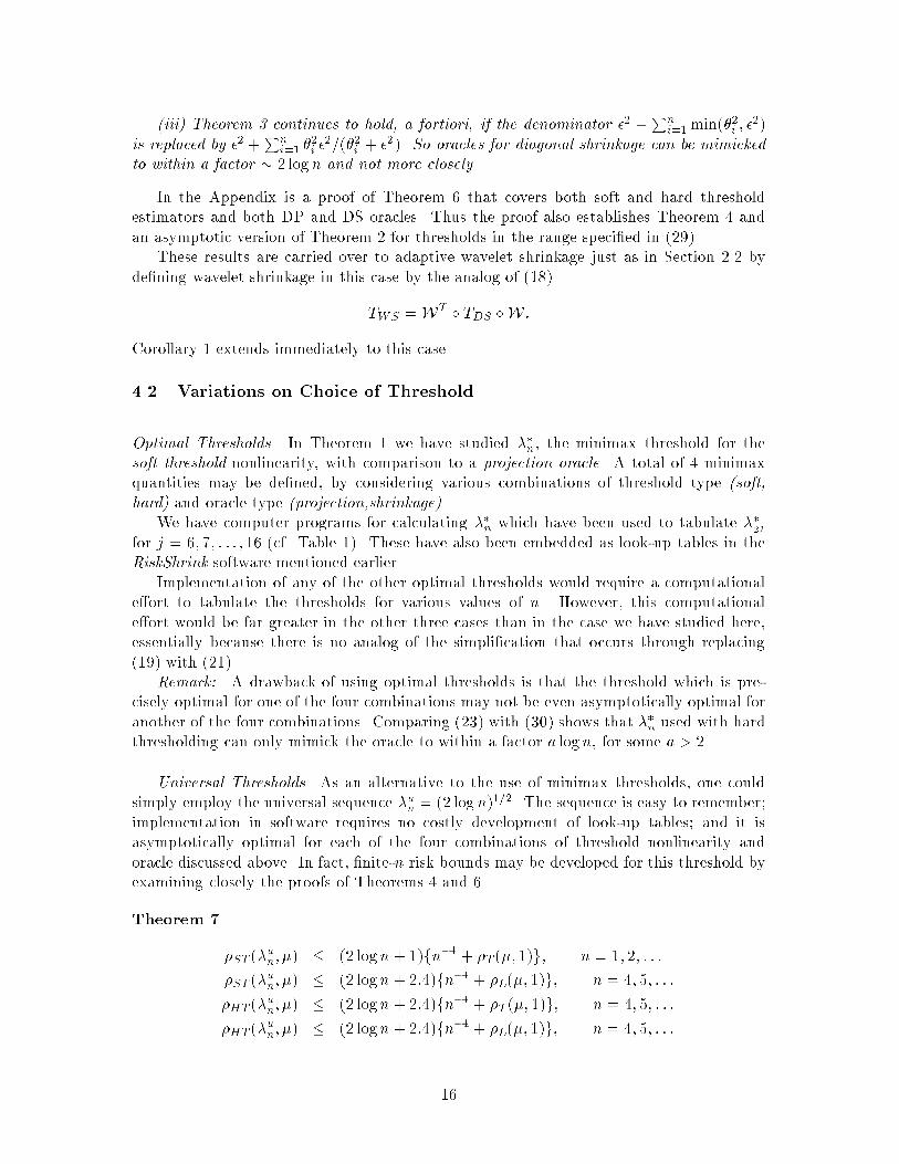
4.2 Variations on Choice of Threshold
Optimal Thresholds. In Theorem 1 we have studied ��
n, the minimax threshold for the
soft threshold nonlinearity, with comparison to a projection oracle. A total of 4 minimax
quantities may be de�ned, by considering various combinations of threshold type (soft,
hard) and oracle type (projection,shrinkage).
We have computer programs for calculating ��n which have been used to tabulate ��2j
for j = 6; 7; : : : ; 16 (cf. Table 1). These have also been embedded as look-up tables in the
RiskShrink software mentioned earlier.
Implementation of any of the other optimal thresholds would require a computational
e�ort to tabulate the thresholds for various values of n. However, this computational
e�ort would be far greater in the other three cases than in the case we have studied here,
essentially because there is no analog of the simpli�cation that occurs through replacing
(19) with (21).
Remark: A drawback of using optimal thresholds is that the threshold which is pre-
cisely optimal for one of the four combinations may not be even asymptotically optimal for
another of the four combinations. Comparing (23) with (30) shows that ��n used with hard
thresholding can only mimick the oracle to within a factor a logn, for some a > 2.
Universal Thresholds. As an alternative to the use of minimax thresholds, one could
simply employ the universal sequence �un = (2 logn)1=2. The sequence is easy to remember;
implementation in software requires no costly development of look-up tables; and it is
asymptotically optimal for each of the four combinations of threshold nonlinearity and
oracle discussed above. In fact, �nite-n risk bounds may be developed for this threshold by
examining closely the proofs of Theorems 4 and 6.
Theorem 7
�ST (�un; �) � (2 logn + 1)fn�1 + �T (�; 1)g; n = 1; 2; : : :
�ST (�un; �) � (2 logn + 2:4)fn�1 + �L(�; 1)g; n = 4; 5; : : :
�HT (�un; �) � (2 logn + 2:4)fn�1 + �T (�; 1)g; n = 4; 5; : : :
�HT (�un; �) � (2 logn + 2:4)fn�1 + �L(�; 1)g; n = 4; 5; : : :
16
The drawback of this simple threshold formula is that in samples on the order of dozens
or hundreds, the mean square error performance of minimax thresholds is noticeably better.
VisuShrink. On the other hand (�un) has an important visual advantage: the almost
\noise-free" character of reconstructions. This can be explained as follows. The wavelet
transform of many noiseless objects, such as those portrayed in �gure 1, is very sparse, and
�lled with essentially zero coe�cients. After contamination with noise, these coe�cients
are all nonzero. If a sample that in the noiseless case ought to be zero is in the noisy
case nonzero, and that character is preserved in the reconstruction, the reconstruction will
have an annoying visual appearance { it will contain small blips against an otherwise clean
background.
The threshold (2 logn)1=2 avoids this problem because of the fact that when (zi) is a
white noise sequence i.i.d. N(0; 1), then
prfmaxijzij > (2 logn)1=2g ! 0; n!1: (31)
So, with high probability, every sample in the wavelet transform in which the underlying
signal is exactly zero will be estimated as zero.
Figure 9 displays the results of using this threshold on the noisy data of Figures 3 and
4. The almost \noise free" character of the plots is striking.
De�nition 2 Let ~�v denote the estimator in the wavelet domain obtained by
~�v =
(wj;k j < j0
�S(wj;k; �(2 logn)1=2) j0 � j � J
:
VisuShrink is the estimator~fvn � W
T� ~�v �W :
Not only is the method better in visual quality than RiskShrink, the asymptotic risk
bounds are no worse:
R( ~fvn ; f) � (2 logn + 1)f�2
n+Rn;�(gSW; f)g:
This estimator is discussed further in our report [asymp.tex].
Estimating the Noise Level. Our software estimates the noise level � as the median
absolute deviation of the wavelet coe�cients at the �nest level J , divided by :6745. In our
experience, the empirical wavelet coe�cients at the �nest scale are, with a small fraction
of exceptions, essentially pure noise. Naturally, this is not perfect; we get an estimate
that su�ers an upward bias due to the presence of some signal at that level. By using the
median absolute deviation, this bias is e�ectively controlled. Incidentally, upward bias is
not disastrous; if our estimate is biased upwards by, say 50%, then the same type of risk
bounds hold, but with with a 3 logn in place of 2 logn.
4.3 Adaptation in Other Bases
A considerable amount of Soviet literature in the 1980's { for example, Efroimovich and
Pinsker (1984) et seq. { concerns what in our terms could be called mimicking an oracle in
the Fourier basis. Our work is an improvement in two respects:
17
1. For the type of objects considered here, a Wavelet Oracle is more powerful than a
Fourier Oracle. Indeed, a Fourier oracle can never give a rate of convergence faster
than n�1=2 on any discontinuous object, while the Wavelet oracle can achieve rates
as fast as logn=n on certain discontinuous objects. Figure 10 displays the results of
using a Fourier-domain oracle with our four basic functions; this should be compared
with Figure 5. Evidently, the Wavelet oracle is visually better in every case. It is also
better in mean square.
2. The Efroimovich-Pinsker work did not have access to the oracle inequality and used
a di�erent approach, not based on thresholding but instead on grouping in blocks
and adaptive linear damping within blocks. Such an approach cannot obey the same
risk bounds as the oracle inequality, and can easily be o� of ideal risk by larger than
logarithmic factors. Indeed, from a \minimax over L2-Sobolev balls" point of view,
for which the Efroimovich-Pinsker work was designed, the adaptive linear damping is
essentially optimal; compare comments in our report [ausws.tex, Section 4]. Actual
reconstructions by RiskShrink and by the Efroimovich-Pinsker method on the data of
Figure 3 show that RiskShrink is much better for spatial adaptation; see Figure 4 of
[ausws.tex].
4.4 Numerical measures of �t
Table 2 contains the average (over location) squared error of the various estimates from our
four test functions for the noise realisation and the reconstructions shown in Figures 2 - 10.
It is apparent that the ideal wavelets reconstruction dominates ideal Fourier and that the
genuine estimate using soft threshold at ��n comes well within the factor 6.824 of the ideal
error predicted for n = 2048 by Table 1. Although the (2 logn)1=2 threshold is visually
preferable in most cases, it has uniformly worse squared error than ��n, which re ects the
well-known divergence between the usual numerical and visual assessments of quality of �t.
Table 3 shows the results of a very small simulation comparison of the same four tech-
niques as sample size is varied dyadically from n = 256 through 8192, and using 10 replica-
tions in each case. The same features noted in Table 2 extend to the other sample sizes. In
addition, one notes that, as expected, the average squared errors decline more rapidly with
sample size for the smoother signals HeaviSine and Doppler than for the rougher Blocks
and Bumps .
4.5 Other Adaptive Properties
The estimator proposed here has a number of optimality properties in minimax decision
theory. In recent work, we consider the problem of estimating f at a single point f(t0)
is discussed, where we believe that f is in some H�older class, but we are not sure of the
exponent nor the constant of the class. RiskShrink is adaptive in the sense that it achieves,
within a logarithmic factor, the best risk bounds that could be had if the class were known;
and the logarithmic factor is necessary when the class is unknown, by work of Brown and
Low (1993) and Lepskii (1990). Other near-minimax properties are described in detail in
our report [asymp.tex].
18
4.6 Boundary correction
As described in the Introduction, Cohen, Daubechies, Jawerth and Vial (1993), have intro-
duced separate `boundary �lters' to correct the non-orthogonality on [0; 1] of the restriction
to [0; 1] of basis functions that intersect [0; 1]c. To preserve the important property [W1]
of orthogonality to polynomials of degree �M , a further `preconditioning' transformation
P of the data y is necessary. Thus, the transform may be represented as W = U � P ,
where U is the orthogonal transformation built from the quadrature mirror �lters and their
boundary versions via the cascade algorithm. The preconditioning transformation a�ects
only the N = M + 1 left-most and the N right-most elements of y: it has block diagonal
structure P = diag(PL j I j PR). The key point is that the size and content of the boundary
blocks PL and PR do not depend on n = 2J+1. Thus the Parseval relation (17) is modi�ed
to
1jj�jj22;n � jjf jj
22;n � 2jj�jj
22;n;
where the constants i correspond to the smallest and largest singular values of PL and
PR, and hence do not depend on n = 2J+1. Thus all the ideal risk inequalities in the
paper remain valid, with only an additional dependence for the constants on 1 and 2. In
particular, the conclusions concerning logarithmic mimicking of oracles are unchanged.
4.7 Relation to Model Selection
RiskShrink may be viewed by statisticians as an automatic model selection method, which
picks a subset of the wavelet vectors and �ts a \model", consisting only of wavelets in
that subset, to the data by ordinary least-squares. Our results show that the method
gives almost the same performance in mean-square error as one could attain if one knew in
advance which model provided the minimum mean-square error.
Our results apply equally well in orthogonal regression. Suppose we have Y = X�+E,
with noise Ei independent and identically distributed as N(0; �2), and X an n by p matrix.
Suppose that the predictor variables are orthogonal: XTX = Ip. Theorem 1 shows that
the estimator ~�� = ��� X
TY achieves a risk not worse than p�1 + Rp;�(DP; �) by more
than a factor 2 log p + 1. This point of view has amusing consequences. For example, the
hard thresholding estimator ~�+ = �+� X
TY amounts to \backwards-deletion" variable
selection; one retains in the �nal model only variables which had Z-scores larger than �
in the original least-squares �t of the full model. In small dimensions p, this actually
corresponds to current practice; the \5% signi�cance" rule � � 2 is near-minimax, in the
sense of Theorem 2, for p � 200.
For lack of space, we do not pursue the model-selection connection here at length, except
for two comments.
1. George and Foster (1990) have proved two results about model selection which it
is interesting to compare with our Theorem 4. In our language, they show that
one can mimick the \nonzeroness" oracle �Z(�; �) = �21
f� 6=0g to within Ln = 1 +
2 log(n + 1) by hard thresholding with �n = (2 log(n + 1))1=2. They also show that
for what we call the hard thresholding nonlinearity, no other choice of threshold can
give a worst-case performance ratio, which they call a \Variance In ation Factor",
asymptotically smaller than � 2 logn as n ! 1. Compare also Bickel(1983). Our
results here di�er because we attempt to mimick more powerful oracles, which attain
optimal mean-squared errors. The increase in power of our oracles is expressed by
19
�Z(�; 1)=�L(�; 1) ! 1 as � ! 0. Intuitively, our oracles achieve signi�cant risk
savings over the nonzeroness oracle for the case when the true parameter vector has
many coordinates which are nearly, but not precisely zero. We thank Dean Foster
and Ed George for calling our attention to this interesting work, which also describes
connections with \classical" model selection, such as Gideon Schwarz' BIC criterion.
2. Alan Miller (1984, 1990) has described a model selection procedure whereby an equal
number of \pure noise variables", namely column vectors independent of Y , are ap-
pended to the X matrix. One stops adding terms into the model at the point where
the next term to be added would be one of the arti�cial, pure noise variables. This
simulation method sets, implicitly, a threshold at the maximum of a collection of n
Gaussian random variables. In the orthogonal regression case, this maximum behaves
like (2 logn)1=2, i.e. (�un) (compare (31)). Hence Miller's method is probably not far
from minimaxity with respect to an MSE-oracle.
ACKNOWLEDGEMENTS
This paper was completed while Donoho was on leave from the University of California,
Berkeley, where this work was supported by grants from NSF and NASA. Johnstone was
supported in part by grants from NSF and NIH. Helpful comments of a referee are gratefully
acknowledged. We are also most grateful to Carl Taswell, who carried out the simulations
reported in Table 3.
5 Appendix: Proofs
5.1 Proof of Theorem 1
It is enough to verify the univariate case, for the multivariate case follows by summation.
So, let X � N(�; 1), and �t(x) = sgn(x)(jxj � t)+. In fact we show, for all � � 1=2 and
with t = (2 log ��1)1=2 that
E(�t(X)� �)2 � (2 log ��1 + 1)(� + �2^ 1):
Regard the right side above as the minimum of two functions and note �rst that
E(�t(X)� �)2 = 1� 2pr�(jX j < t) +E� X2^ t
2� 1 + t
2 (32)
� (2 log ��1 + 1)(� + 1);
where we used X2^ t
2� t
2. Using instead X2^ t
2� X
2, we get from (32)
E(�t� �)2� 2pr�(jX j � t) + �
2: (33)
The proof will be complete if we verify that
g(�) = 2pr�(jX j � t) � �(2 log ��1 + 1) + (2 log ��1)�2:
Since g is symmetric about 0,
g(�) � g(0)+ (1=2)(sup jg00j)�2: (34)
Finally, some calculus shows that g(0) = 4�(�t) � �(2 log ��1 + 1) and that sup jg00j �
4 sup jx�(x)j � 4 log ��1 for all � � 1=2.
20
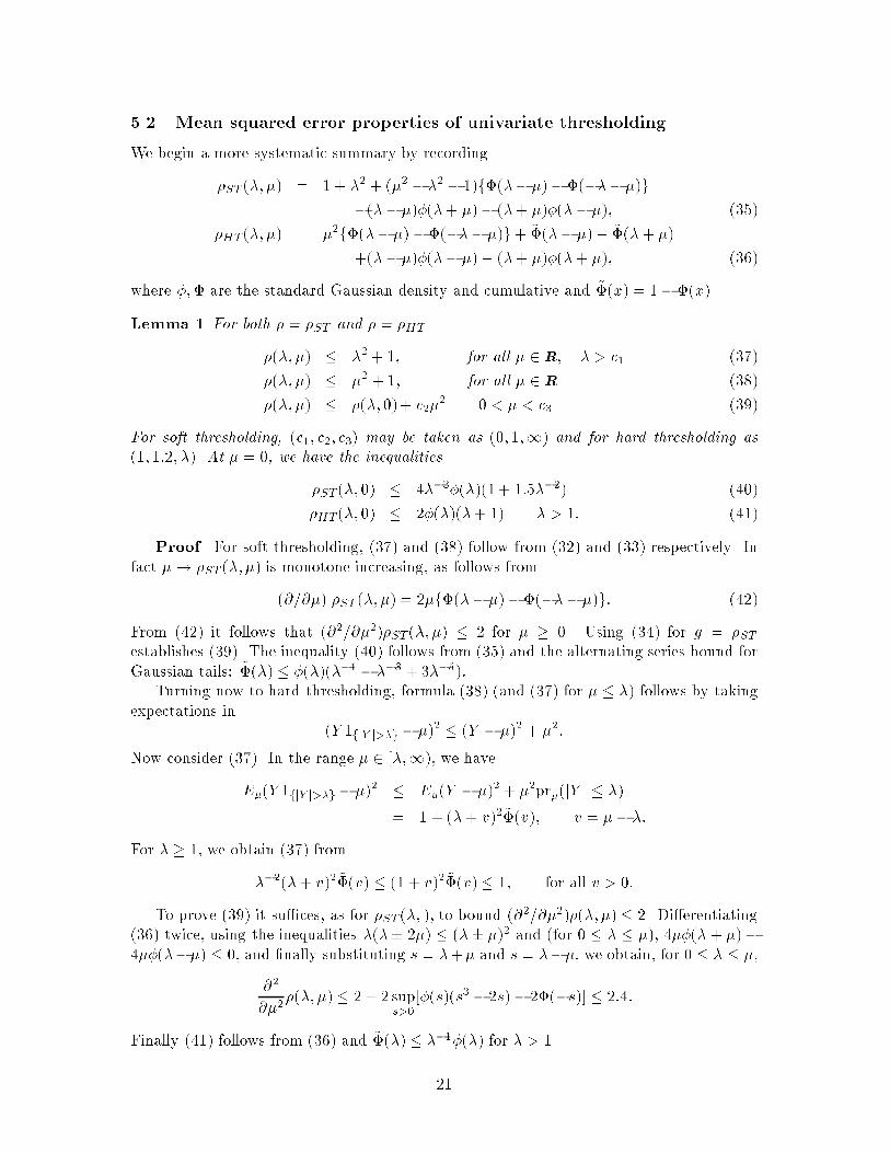
5.2 Mean squared error properties of univariate thresholding.
We begin a more systematic summary by recording
�ST (�; �) = 1 + �2 + (�2 � �2 � 1)f�(�� �)� �(��� �)g
�(�� �)�(�+ �)� (�+ �)�(�� �); (35)
�HT(�; �) = �2f�(�� �) � �(��� �)g+ ~�(�� �) + ~�(�+ �)
+(�� �)�(�� �) + (�+ �)�(�+ �); (36)
where �;� are the standard Gaussian density and cumulative and ~�(x) = 1� �(x).
Lemma 1 For both � = �ST and � = �HT
�(�; �) � �2 + 1; for all � 2 R; � > c1 (37)
�(�; �) � �2 + 1; for all � 2 R (38)
�(�; �) � �(�; 0)+ c2�2 0 < � < c3 (39)
For soft thresholding, (c1; c2; c3) may be taken as (0; 1;1) and for hard thresholding as
(1; 1:2; �). At � = 0, we have the inequalities
�ST (�; 0) � 4��3�(�)(1+ 1:5��2) (40)
�HT(�; 0) � 2�(�)(�+ 1) � > 1: (41)
Proof. For soft thresholding, (37) and (38) follow from (32) and (33) respectively. In
fact �! �ST (�; �) is monotone increasing, as follows from
(@=@�) �ST (�; �) = 2�f�(�� �)� �(��� �)g: (42)
From (42) it follows that (@2=@�2)�ST (�; �) � 2 for � � 0. Using (34) for g = �ST
establishes (39). The inequality (40) follows from (35) and the alternating series bound for
Gaussian tails: ~�(�) � �(�)(��1 � ��3 + 3��5):
Turning now to hard thresholding, formula (38) (and (37) for � � �) follows by taking
expectations in
(Y 1fjY j>�g � �)2 � (Y � �)2 + �
2:
Now consider (37). In the range � 2 [�;1), we have
E�(Y 1fjY j>�g � �)2 � E�(Y � �)2 + �2pr�(jY j � �)
= 1 + (�+ v)2~�(v); v = � � �:
For � � 1, we obtain (37) from
��2(�+ v)2 ~�(v) � (1 + v)2~�(v) � 1; for all v > 0:
To prove (39) it su�ces, as for �ST (�; ), to bound (@2=@�2)�(�; �) � 2. Di�erentiating
(36) twice, using the inequalities �(�� 2�) � (�� �)2 and (for 0 � � � �), 4��(�+ �)�
4��(���) � 0, and �nally substituting s = �+� and s = ���, we obtain, for 0 � � � �,
@2
@�2�(�; �) � 2 + 2 sup
s>0[�(s)(s3 � 2s)� 2�(�s)] � 2:4:
Finally (41) follows from (36) and ~�(�) � ��1�(�) for � > 1.
21
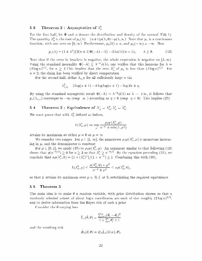
5.3 Theorem 2 : Asymptotics of �0n
For the �rst half, let � and � denote the distribution and density of the normal N(0; 1).
The quantity �0n is the root of pn(�) = (n+1)�(�; 0)��(�;1). Note that pn is a continuous
function, with one zero on [0;1). Furthermore, pn(0) = n, and pn(+1) = �1. Now
pn(�) = (1 + �2)f2(n+ 1)�(��)� 1g � 2��(�)(n+ 1); � � 0: (43)
Note that if the term in brackets is negative, the whole expression is negative on [�;1).
Using the standard inequality �(��) � ��1�(�), one veri�es that this happens for � =
(2 logn)1=2, for n � 3.This implies that the zero �0n of pn is less than (2 logn)1=2. For
n = 2, the claim has been veri�ed by direct computation.
For the second half, de�ne ��;N for all su�ciently large n via
�2�;n = 2 log(n+ 1)� 4 log log(n+ 1)� log 2� + �:
By using the standard asymptotic result �(��) � ��1�(�) as � ! +1, it follows that
pn(��;n) converges to �1 (resp. 1 ) according as � > 0 (resp. � < 0). This implies (23).
5.4 Theorem 2 : Equivalence of ��
n = �0n; �
�
n = �0n:
We must prove that with �0n de�ned as before,
L(�0n; �) := sup�
�ST (�0n; �)
n�1 +min(1; �2)
attains its maximum at either � = 0 or � =1.
We consider two ranges. For � 2 [1;1], the numerator �ST (�0n; �) is monotone increas-
ing in �, and the denominator is constant.
For � 2 [0; 1], we apply (39) to �ST (�0n; �). An argument similar to that following (43)
shows that p(n�1=2) � 0 for n � 3 so that �0n � n�1=2. By the equation preceding (22), we
conclude that n�(�0n; 0) = f1 + (�0n)2g=(1 + n
�1) � 1. Combining this with (39),
L(�0n; �) ��(�0n; 0) + �
2
n�1 + �2� n�(�0n; 0);
so that L attains its maximum over � 2 [0; 1] at 0, establishing the required equivalence.
5.5 Theorem 3
The main idea is to make � a random variable, with prior distribution chosen so that a
randomly selected subset of about logn coordinates are each of size roughly (2 logn)1=2,
and to derive information from the Bayes risk of such a prior.
Consider the �-varying loss
~Ln(�̂; �) =
Pni=1(�̂i � �i)
2
1 +P
i �2i ^ 1
and the resulting risk~Rn(�; �) = E�
~Ln(�(w); �):
22
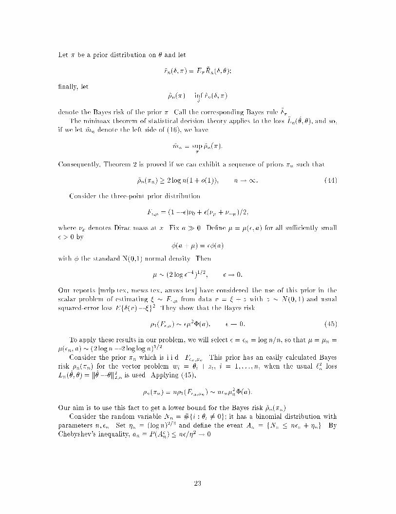
Let � be a prior distribution on � and let
~rn(�; �) = E�~Rn(�; �);
�nally, let
~�n(�) = inf�~rn(�; �)
denote the Bayes risk of the prior �. Call the corresponding Bayes rule ~�� .
The minimax theorem of statistical decision theory applies to the loss ~Ln(�̂; �), and so,
if we let ~mn denote the left side of (16), we have
~mn = sup�
~�n(�):
Consequently, Theorem 2 is proved if we can exhibit a sequence of priors �n such that
~�n(�n) � 2 logn(1 + o(1)); n!1: (44)
Consider the three-point prior distribution
F�;� = (1� �)�0 + �(�� + ���)=2;
where �x denotes Dirac mass at x. Fix a � 0. De�ne � = �(�; a) for all su�ciently small
� > 0 by
�(a+ �) = ��(a)
with � the standard N(0,1) normal density. Then
� � (2 log ��1)1=2; �! 0:
Our reports [mrlp.tex, mews.tex, ausws.tex] have considered the use of this prior in the
scalar problem of estimating � � F�;� from data v = � + z with z � N(0; 1) and usual
squared-error loss Ef�(v)� �g2. They show that the Bayes risk
�1(F�;�) � ��2�(a); � ! 0: (45)
To apply these results in our problem, we will select � = �n = log n=n, so that � = �n =
�(�n; a) � (2 logn� 2 log log n)1=2.
Consider the prior �n which is i.i.d. F�n;�n . This prior has an easily calculated Bayes
risk �n(�n) for the vector problem wi = �i + zi, i = 1; : : : ; n, when the usual `2n loss
Ln(�̂; �) = k�̂ � �k22;n is used. Applying (45),
�n(�n) = n�1(F�n;�n) � n�n�2n�(a):
Our aim is to use this fact to get a lower bound for the Bayes risk ~�n(�n).
Consider the random variable Nn = #fi : �i 6= 0g; it has a binomial distribution with
parameters n; �n. Set �n = (logn)2=3 and de�ne the event An = fNn � n�n + �ng. By
Chebyshev's inequality, an � P (Acn) � n�=�
2! 0.
23
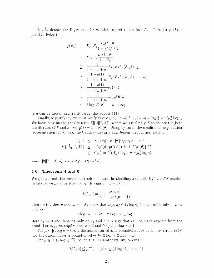
Let ~�n denote the Bayes rule for �n with respect to the loss ~Ln. Then (step (*) is
justi�ed below)
~�(�n) = E�nE�Ln(~�n; �)
1 +P�2i ^ 1
= E�nE�Ln(~�n; �)
1 +Nn
�1
1 + n�n + �nE�nE�Ln(~�n; �)1An
�1 + o(1)
1 + n�n + �nE�nE�Ln(~�n; �) (�)
�1 + o(1)
1 + n�n + �n
�n(�n)
�1
1 + n�n + �nn�n�
2�(a)
� 2 logn�(a) n!1;
as a can be chosen arbitrarily large, this proves (44).
Finally, to justify (*), we must verify thatE�nE�[jj~���jj2; A
cn] = of�n(�n)g = o(�2n logn):
We focus only on the trickier term E[jj~�jj2; Acn], where we use simply E to denote the joint
distribution of � and x. Set p(�) = 1 +Nn(�). Using by turns the conditional expectation
representation for ~�n;i(x), the Cauchy-Schwartz and Jensen inequalities, we �nd
jj~�njj2� E[p(�)jx]E[jj�jj2=p(�)jx]; and
Efjj~�njj2; A
cng � fEp
4(�) pr2(Acn) Ejj�jj
8=p
4(�)g1=4
� C�2n pr1=2(Ac
n) logn = o(�2n logn);
since jj�jj8 = Nn�8n and ENp
n = O(logp n).
5.6 Theorems 4 and 6
We give a proof that covers both soft and hard thresholding, and both DP and DS oracles.
In fact, since �L < �T it is enough to consider � = �L. Let
L(�; �) =�(�; �)
n�1 + �2=(�2 + 1);
where � is either �ST or �HT . We show that L(�; �) � (2 logn)(1 + �n) uniformly in � so
long as
c log logn � �2� 2 logn � �n logn:
Here �n ! 0 and depends only on �n and c in a way that can be made explicit from the
proof. For �ST , we require that c < 5 and for �HT , that c < 1.
For � 2 [(2 logn)1=2;1], the numerator of L is bounded above by 1 + �2 (from (37))
and the denominator is bounded below by 2 logn=(2 logn + 1).
For � 2 [1; (2 logn)1=2], bound the numerator by (38) to obtain
L(�; �) � ��2(1 + �
2)2 � (2 logn)f1 + o(1)g:
24
For � 2 [0; 1], use (39):
L(�; �) �
�(�; 0)
n�1+�(�; �)� �(�; 0)
�2=(1 + �2)
� n�(�; 0)+ 2c2: (46)
If �n(c) = (2 logn � c log log n)1=2, then n�(�n(c)) = �(0)(logn)c=2. It follows from (40)
and (41) that n�(�; 0) and hence L(�; �) = o(logn) if � > �n(c) where c < 5 for soft
thresholding and c < 1 for hard thresholding. The expansion (23) shows that this range
includes ��n and hence �̂�.
5.7 Theorem 7
When �2 = (2 logn)1=2, the bounds over [1; (2 logn)1=2] and [(2 logn)1=2;1] in the previous
section become simply [1 + 2 logn]2=2 logn � 2 logn + 2:4 for n � 4. For � 2 [0; 1], the
bounds follow by direct evaluation from (46), (40) and (41). We note that these bounds
can be improved slightly by considering the cases separately.
References
[1] BICKEL, P. J. (1983). Minimax estimation of a normal mean subject to doing well at
a point. In Recent Advances in Statistics (M. H. Rizvi, J. S. Rustagi, and D. Siegmund,
eds.), Academic Press, New York, 511{528.
[2] BREIMAN, L., FRIEDMAN, J.H., OLSHEN, R.A.,& STONE, C.J. (1983). CART:
Classi�cation and Regression Trees . Wadsworth: CBelmont, CA.
[3] BROCKMANN, M., GASSER, T., & HERRMANN, E. (1992). Locally Adaptive
Bandwidth Choice for Kernel Regression Estimators. To appear. J. Amer. Statist.
Assoc..
[4] BROWN, L.D. & LOW, M.G. (1993). Supere�ciency and lack of adaptability in non-
parametric functional estimation. To appear, Annals of Statistics.
[5] COHEN, A., DAUBECHIES, I., JAWERTH, B. & VIAL, P. (1993). Multiresolution
analysis, wavelets, and fast algorithms on an interval. Comptes Rendus Acad. Sci. Paris
(A). 316., 417{421.
[6] CHUI, C.K. (1992)., An Introduction to Wavelets. Academic Press, Boston, MA.
[7] DAUBECHIES, I. (1988). Orthonormal bases of compactly supported wavelets. Com-
munications in Pure and Applied Mathematics 41, Nov. 1988, pp. 909-996.
[8] DAUBECHIES, I. (1992). Ten Lectures on Wavelets SIAM: Philadelphia.
[9] DAUBECHIES, I. (1993). Orthonormal Bases of Compactly Supported Wavelets II:
Variations on a theme. SIAM J. Math. Anal., 24, 499{519.
[10] EFROIMOVICH, S. YU. & PINSKER, M.S. (1984). A learning algorithm for non-
parametric �ltering. Automat. i Telemeh. 11 58-65 (in Russian).
25
[11] FRAZIER M., JAWERTH B., & WEISS G. (1991). Littlewood-Paley Theory and the
study of function spaces.NSF-CBMS Regional Conf. Ser in Mathematics, 79. American
Math. Soc.: Providence, RI.
[12] FRIEDMAN, J.H. & SILVERMAN, B.W. (1989). Flexible Parsimonious Smoothing
and Additive Modeling. (with discussion). Technometrics 31, 3{39.
[13] FRIEDMAN, J.H. (1991). Multiple Additive Regression Splines (with discussion). An-
nals of Statistics, 19, 1{67.
[14] GEORGE, E. I. & Foster, D. P.(1990). The risk in ation of variable selection in re-
gression. Technical Report, University of Chicago.
[15] LEPSKII, O.V. (1990). On one problem of adaptive estimation on white Gaussian
noise. Teor. Veoryatnost. i Primenen. 35 459-470 (in Russian). Theory of Probability
and Appl. 35, 454-466 (in English).
[16] MALGOUYRES, G. (1991). Ondelettes sur l'Intervalle: algorithmes rapides.
Pr�epublications Mathematiques Orsay.
[17] MEYER, Y. (1990). Ondelettes et Op�erateurs: I. Ondelettes Hermann et Cie, Paris.
[18] MEYER, Yves (1991). Ondelettes sur l'intervalle. Revista Matem�atica Ibero-Americana
7 (2), 115-133.
[19] MILLER, A.J. (1984). Selection of subsets of regression variables (with discussion). J.
R. Statist. Soc. A., 147,389{425.
[20] MILLER, A.J. (1990). Subset Selection in Regression. Chapman and Hall. London,
New York.
[21] M�ULLER, Hans-Georg & STADTMULLER, Ulrich. (1987). Variable bandwidth kernel
estimators of regression curves. Ann. Statist., 15(1), 182{201.
[22] TERRELL, G.R. & SCOTT, D.W. (1992). Variable kernel density estimation. Annals
of Statistics., 20, 1236 { 1265.
26
Table 1
��
n and Related Quantities
n ��
n (2 logn)1=2 ��n 2 logn+ 1
64 1.474 2.884 3.124 8.3178
128 1.669 3.115 3.755 9.7040
256 1.860 3.330 4.442 11.090
512 2.048 3.532 5.182 12.477
1024 2.232 3.723 5.976 13.863
2048 2.414 3.905 6.824 15.249
4096 2.594 4.079 7.728 16.635
8192 2.773 4.245 8.691 18.022
16384 2.952 4.405 9.715 19.408
32768 3.131 4.560 10.80 20.794
65536 3.310 4.710 11.95 22.181
27
Table 2
average square errors jjf̂ � f jj22;n=n in the Figures
Figure Blocks Bumps HeaviSine Doppler
Fig 1: jjf jj22;n=n 81.211 57.665 52.893 50.348
Fig 3: with noise 1.047 0.937 1.008 0.9998
Fig 5: ideal wavelets 0.097 0.111 0.028 0.042
Fig 10: ideal Fourier 0.370 0.375 0.062 0.200
Fig 7: threshold ��n 0.395 0.496 0.059 0.152
Fig 9: threshold (2 logn)1=2 0.874 1.058 0.076 0.324
28
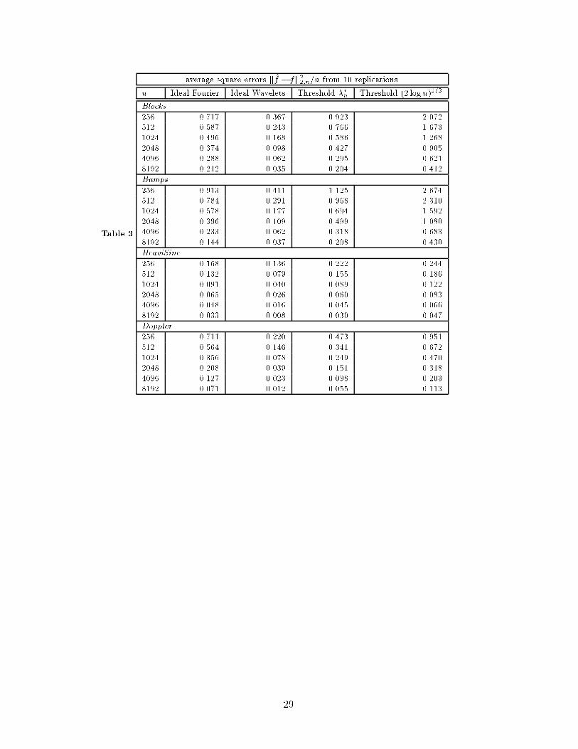
Table 3
average square errors jjf̂ � f jj22;n=n from 10 replications
n Ideal Fourier Ideal Wavelets Threshold ��n Threshold (2 log n)1=2
Blocks
256 0.717 0.367 0.923 2.072
512 0.587 0.243 0.766 1.673
1024 0.496 0.168 0.586 1.268
2048 0.374 0.098 0.427 0.905
4096 0.288 0.062 0.295 0.621
8192 0.212 0.035 0.204 0.412
Bumps
256 0.913 0.411 1.125 2.674
512 0.784 0.291 0.968 2.310
1024 0.578 0.177 0.694 1.592
2048 0.396 0.109 0.499 1.080
4096 0.233 0.062 0.318 0.683
8192 0.144 0.037 0.208 0.430
HeaviSine
256 0.168 0.136 0.222 0.244
512 0.132 0.079 0.155 0.186
1024 0.091 0.040 0.089 0.122
2048 0.065 0.026 0.060 0.083
4096 0.048 0.016 0.045 0.066
8192 0.033 0.008 0.030 0.047
Doppler
256 0.711 0.220 0.473 0.951
512 0.564 0.146 0.341 0.672
1024 0.356 0.078 0.249 0.470
2048 0.208 0.039 0.151 0.318
4096 0.127 0.023 0.098 0.203
8192 0.071 0.012 0.055 0.113
29
List of Figures
1. Four spatially variable functions. n=2048. Formulas below.
2. The four functions in the wavelet domain. Most Nearly Symmetric Daubechies
Wavelet with N = 8 was used. Wavelet Coe�cients �j;k are depicted for j =
5; 6; : : : ; 10. Coe�cients in one level (j constant) are plotted as a series against posi-
tion t = 2�jk. The vast majority of the coe�cients are zero or e�ectively zero.
3. Four functions with Gaussian white noise, � = 1, rescaled to have signal-to-noise
ratio, SD(f)=� = 7.
4. The four noisy functions in the wavelet domain. Compare Fig. 2. Only a small
number of coe�cients stand out against a noise background.
5. Ideal Selective Wavelet Reconstruction, with j0 = 5. Compare Figs. 1,3.
6. Ideal Reconstruction, Wavelet Domain. Compare Figs. 2,4. Most of the coe�cients
in Figure 4 have been set to zero. The others have been retained as is.
7. RiskShrink Reconstruction using soft thresholding and � = ��
n. Mimicking an oracle
while relying on the data alone.
8. RiskShrink, Wavelet Domain. Compare Figs 2,4,6.
9. VisuShrink reconstructions using soft thresholding and � = (2 logn)1=2. Notice
\noise-free" character; compare Figs 1,3,5,7.
10. Ideal Selective Fourier Reconstruction. Compare Fig. 5. Superiority of Wavelet
Oracle is evident.
Formulas for Test Functions
Blocks.
f(t) =X
hjK(t� tj) K(t) = (1 + sgn(t))=2:
(tj) = (:1; :13; :15; :23; :25; :40; :44; :65; :76; :78; :81)
(hj) = (4; �5; 3; �4; 5; �4:2; 2:1; 4:3; �3:1; 5:1; �4:2)
Bumps.
f(t) =X
hjK((t� tj)=wj) K(t) = (1 + jtj4)�1:
(tj) = tBlocks
(hj) = (4; 5; 3; 4; 5; 4:2; 2:1; 4:3; 3:1; 5:1; 4:2)
(wj) = (:005; :005; :006; :01; :01; :03; :01; :01; :005; :008; :005)
HeaviSine.
f(t) = 4 sin 4�t� sgn(t� :3)� sgn(:72� t):
Doppler.
f(t) = (t(1� t))1=2 sin(2�(1 + �)=(t+ �)); � = :05:
30