Transportation Research Record 948 63

Hydraulic Design of Stormwater Pumping Stations: The Effect of Storage ROBERT H. BAUMGARDNER

In the design of stormwater pumping stations, skillful design can reduce both the initial cost and operating costs. The initial cost can be reduced by provid­ing storage to reduce the peak pump rate. Savings can be achieved by reducing the size of the pump, the pump motor, piping, and valves, and substantial savings can accrue if the number of pumps is reduced. Most electrical utilities assess a fixed charge for the electrical capacity that the utility must maintain to provide service. Because horsepower is directly proportional to the pump­ing rate, any reduction in the pumping rate will be reflected in the fixed charge. By providing storage to reduce the peak pumping rate, operating costs can be considerably reduced. The effect of storage can be evaluated by using a mass curve routing procedure. This design procedure combines three independent components-the inflow hydrograph, the stage-storage relationship, and the stage-discharge relationship. The mass curve routing procedure identi­fies the amount of storage required to reduce the peak rate of flow to the fixed discharge rate. Design guidance is also provided for estimating the amount of storage required to accomplish a given reduction, and formulas are provided for calculating the volume of storage basins.

In most localities stormwater pumping stations only operate for a relatively short period of time during a year. This means that a substantial capital in­vestment must sit idle for long periods of time. Therefore, the design . and operation of stormwater pumping stations provide a most promising opportu­nity for cost reduction. Potential savings are even more promising in areas where storms are less fre­quent.

The merits of providing storage to reduce the peak pumping rates of pumping stations have long been recognized by engineers. To control the costs of stormwater projects, engineers are now examining potential savings much more closel~. To achieve meaningful cost reductions, savings must be accom­plished in both construction cost and maintenance and operations costs.

Initial costs can be reduced by providing storage to reduce the peak pumping rate: this will produce savings in the cost of the pump, the pump motor, and the instrumentation. Additional savings can be achieved by reducing the size of piping and valves. Substantial savings can accrue if the number of pumps is reduced. These savings will be offset by the cost of providing storage, but in many cases a net savings will occur if the storage can be pro"­vided at a low cost.

Maintenance and operating costs can be lowered by reducing the fixed electrical charge assessed by most electrical utilities. This charge is basically for the electrical capacity that the utility must maintain to service the pumping station and is usually proportional to the horsepower of the sta­tion. Because the horsepower is directly propor­tional to the pumping rate, any reduction in the pumping rate will be reflected in the fixed electri­cal charge.

This paper provides design guidance for s1z1ng storage facilities used to reduce peak rates of flow at stormwater pumping stations.

DESIGN PROCEDURE

The merits of using storage to reduce peak flows are illustrated here by using a generalized case because the case of an actual pumping station may be compli­cated by the varying pumping rates and discontinui-

ties as the pumps turn on and off. This is shown in Figure 1, where the shaded area between the curves represents the volume of stormwater that must be stored to reduce the peak flow rate. Storage exists in natural channels, storm drain systems, con­structed basins or forebays, and storage boxes. Engineers must be able to identify and analyze the effect of stora,ge on the discharge rates from the pumping station.

Designers must establish the interrelationship of three separate components:

1. The inflow hydrograph must be determined for the contributing watershed.

2. The volumetric storage capability of the storage facility must be identified.

3. The stage-discharge curve of the pumps must be determined.

Once these three components have been established, a mass curve routing procedure can be used to analyze the problem.

The mass curve routing procedure is based on the assumption that the storage facility acts as a reservoir. Figure 2 helps to illustrate two short­comings of this assumption. First, the velocity in the pipe is not zero (this shortcoming should be minor because the velocities should be low). Second, the water depth of the reservoir decreases to zero as the water surface approaches the invert of the pipe. During peak flow conditions the pipe will be flowing full and the design conditions shown in Fig­ure 2 will not exist.

The second shortcoming can be eliminated by pro­viding an isolated depressed storage facility that is independent of the storm drain system: however, in most systems it is quite cost effective to use the storm drain system as the storage facility. If a boundary is drawn around the storage facility and

Figure 1. Generalized storage case.

40

30 Flow­cfto 20

10

Inflow hydrograph

Time· hre

Figure 2. Reservoir routing.

1& 19

64

the pumping station so that they act as a unit, the reservoir assumption is valid because the design conditions conform to the general storage equation:

(f - 0) L'>t =L'>S

wher e

I average inflow rate,

0 average outflow rate, 6t time increment, and 6S change in storage.

(I)

The inflow rate is defined by the design hydro­graph, the outflow rate by the pumping discharge rates, and storage by the stage-storage curve. Be­cause Equation 1 is valid inside the boundary, the reservoir assumption is an adequate representation of design conditions.

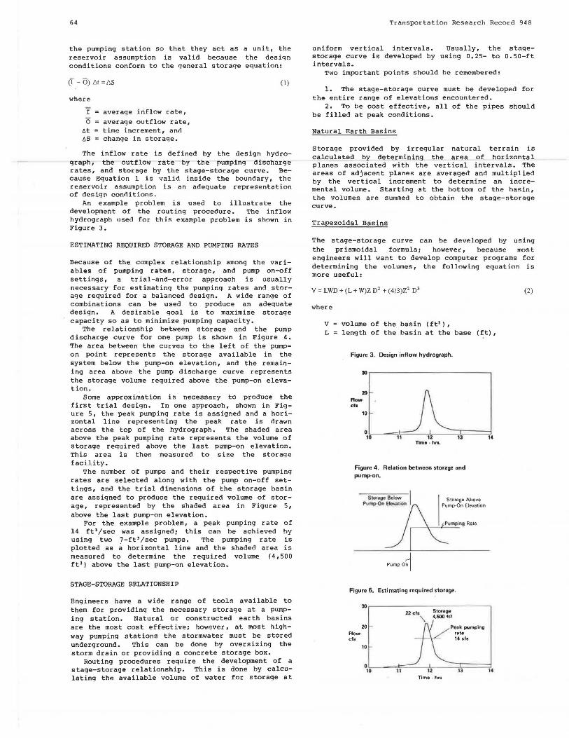
An example problem is used to illustrate the development of the routing procedure. The inflow hydrograph used for this example problem is shown in Figure 3.

ESTIMATING REQUIRED STORAGE AND PUMPING RATES

Because of the complex relationship among the vari­ables; of pumping rates, storage, and pump on-off settings, a trial-and-error approach is usually necessary for estimating the pumping rates and stor­age required for a balanced design. A wide range of combinations can be used to produce an adequate design. A desirable goal is to maximize storage capacity so as to minimize pumping capacity.

The relationship between storage and the pump discharge curve for one pump is shown in Figure 4. The area between the curves to the left of the pump­on point represents the storage available in the system below the pump-on elevation, and the remain­ing area above the pump discharge curve represents the storage volume required above the pump-on eleva­tion.

Some approximation is necessary to produce the first trial design. In one approach, shown in Fig­ure 5, the peak pumping rate is assigned and a hori­zontal line representing the peak rate is drawn across the top of the hydrograph. The shaded area above the peak pumping rate represents the volume of storage required above t.he last pump-on elevation. This area is then measured to size the storage facility.

The number of pumps and their respective pumping rates are selected along with the pump on-off set­tings, and the trial dimensions of the storage basin are assigned to produce the required volume of stor­age, represented by the shaded area in Figure 5, above the last pump-on elevation.

For the example problem, a peak pumping rate of 14 ft'/sec was assigned; this can be achieved by using two 7-ft'/sec pumps. The pumping rate is plotted as a horizontal line and the shaded area is measured to determine the required volume (4,500 ft') above the last pump-on elevation.

STAGE-STORAGE RELATIONSHIP

Engineers have a wide range of tools available to them for providing the necessary storage at a pump­ing station. Natural or constructed earth basins are the most cost effective; however, at most high­way pumping stations the stormwater must be stored underground. This can be done by oversizing the storm drain or providing a concrete storage box.

Routing procedures require the development of a stage-storage relationship. This is done by calcu­lating the available volume of water for storage at

Tr ansportation Re search Record 948

uniform vertical intervals. Usually, the stage­storage curve is developed by using 0.25- to 0.50-ft intervals.

Two important points should be remembered:

1. The stage-storage curve must be developed for the entire range of elevations encountered.

2. To be cost effective, all of the pipes should be filled at peak conditions.

Natural Earth Basins

Storage provided by irregular natural terrain is calculated by determining the area of horizontal planes associated with the vertical intervals. The areas of adjacent planes are averaged and multiplied by the vertical increment to determine an incre­mental volume. Starting at the bottom of the basin, the vol umes are summed to obtain the stage-storage curve.

Trapezoidal Basins

The stage-storage curve can be developed by using the prismoidal formula; however, because most engineers will want to develop computer programs for determining the volumes, the following equation is more useful:

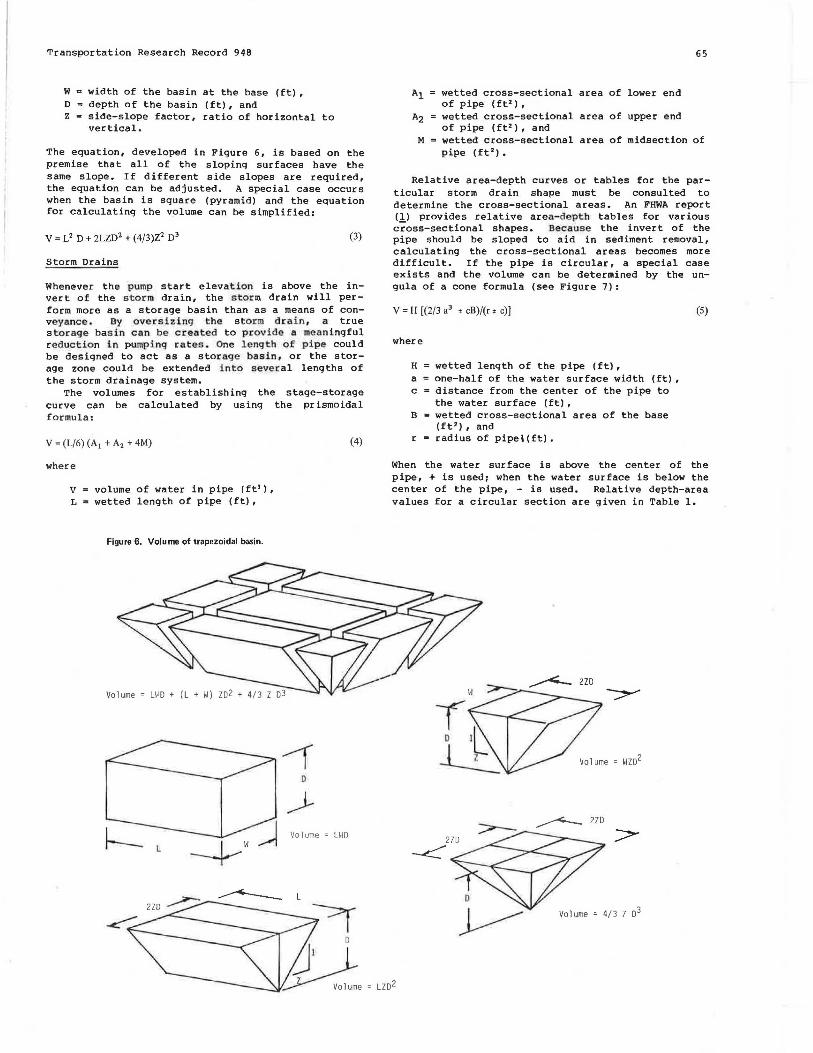
V = LWO + (L + W)Z 0 2 + (4/3)Z2 0 3

where

v L

volume of the basin (ft'), length of the basin at the base (ft),

Figure 3. Design inflow hydrograph.

30

20 Row· ch

10

0 10 11 13

Figure 4. Relation between storage and pump-on.

Stotige Below I Storage Above Pump·On~Elo\iadon Pump-On Elevation

[ ~-"'"

Pump·O~

Figure 5. Estimating required storage.

20 Pt•k pumping Flow· rate els 14 cfs

10

0 10 II 13

Time · hrs

14

,.

(2)

Transportation Research Record 948

W = width of the basin at the base (ft) , D depth of the basin (ft), and z side-slope factor, ratio of horizontal to

vertical.

The equation, developed in Figure 6, is based on the premise that all of the slopinq surfaces have the same slope. If different side slopes are required, the equation can be adjusted. A special case occurs when the basin is square (pyramid) and the equation for calculatinq the volume can be simplified:

V = L2 D + 2LZD2 + (4/3)Z2 D3 (3)

Storm Drains

Whenever the pump start elevation is above the in­vert of the storm drain, the storm drain will per­form more as a storage basin than as a means of con­veyance . By ovezslzing the storm drain, a true storage basin can be created to provide a meaningful r eduction in pumping rates. One lenqth of pipe could be desiqned to act as a storage basin, or the stor­age zone could be extended into seve,ral lengths of the storm drainage system.

The volumes for establishing the stage-storage curve can be calculated by using the prismoidal formula:

V = (L/6) (A 1 + A2 + 4M)

where

v volume of water in pipe (ft'), L = wetted length of pipe (ft) ,

Figure 6. Volume of trapezoidal basin.

(4)

65

Al wetted cross-sectional area of lower end of pipe (ft2 ),

A2 wetted cross-sectional area of upper end of pipe (ft2 ), and

M wetted cross-sectional area of midsection of pipe (ft').

Relative area-depth curves or tables for the par­ticular storm drain shape must be consulted to determine the cross-sectional areas. An FHWA report (1) provides relative area-depth tables for various cross-sectional shapes. Because the invert of the pipe should be sloped to aid in sediment removal, calculating the cross-sectional areas becomes more difficult. If the pipe is circular, a special case exists and the volume can be determined by the un­gula of a cone formula (see Figure 7):

V = H ((2/3 a3 ± cB)/(r ± c))

where

H wetted length of the pipe (ft), a = one-half of the water surface width (ft) , c = distance from the center of the pipe to

the water surface (ft), B wetted cross-sectional area of the base

(ft'), and r = radius of pipel(ft).

(5)

When the water surface is above the center of the pipe, + is usedi when the water surface is below the center of the pipe, - is used. Relative depth-area values for a circular section are given in Table 1.

_...<.- 2ZD

wzo2

_.---<--- 2ZD

2ZD

--<:"

Volume 4/3 7 o3

66

Figure 7. Ungula of a cone.

Stor age Boxes

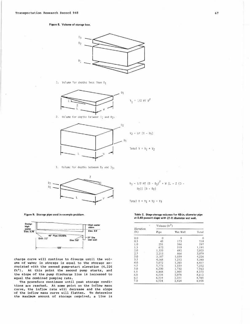
Underground storage boxes would most likely be rec­tangular reinforced concrete boxes. The volumes at the various stages can be calculated by using a com­bination of formulas for regular prisms and triangu­lar wedges. Procedures for determining the volume of storage boxes are provided in Figure 8.

EXAMPLE PROBLEM

In thP. P.Xl'lmple problem, a 520-ft-long, 48-in,-diam eter circular concrete pipe with a 0.40 percent slope is provided as a storage pipe, as shown in Figure 9: a 21- ft-diameter wet well is also pro­vided. The storage volumes for the respective ele­vations are given in Table 2, and the stage-storage curve is plotted in Figure 10.

Stage-Discha rge Relat i onsh i p

Mass curve routing procedures require that a stage­d ischarge relationship be established. For the ex­ample problem presented here, the following staqe­discharge relationship was developed:

Discharge Rate Elevation (ft)

Pump !ft,Lsec} Pump Sta r t Pum;e St o p 1 7 2.0 o.o 2 7 3.0 1.0

This stage-discharge relationship is based on three design assumptions: (a) pump 1 stops at a.o­ft elevation, (b) the pumping ra nge = 2 ft, and (cl there is a 1-ft difference in elevat ion between pump starts.

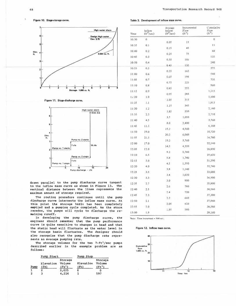
Figure 11 shows the pumping arrangement. Because pumping station design is basically a trial-and-er­ror approach, this pumping arrangement should be considered a first attempt.

Table 1. Relative depth·area values for circular pipes.

c

d/D 0.00 0.01 0.02 0.03 0.04

0.0 0.0013 0.0037 0.0069 0.0105 0.1 0.0409 0.0470 0.0534 0.0600 0.0668 0.2 0.1118 0.1199 0.1281 0.1365 0.1449 0.3 0.1982 0.2074 0.2167 0.2260 0.2355 0.4 0.2934 0.3032 0.3130 0.3229 0.3328 0.5 0.393 0.403 0.413 0.423 0.433 0.6 0.492 0.502 0.512 0.521 0.531 0.7 0.587 0.596 0.605 0.614 0.623 0.8 0.674 0.681 0.689 0.697 0.704 0.9 0.745 0.750 0.756 0.761 0.766 1.0 0.785

Transportation Research Record 948

INFLOW MASS CURVE

To obtain an inflow mass curve, the inflow rates at the limits of a time increment are averaged and mul­tiplied by the time increment to obtain an incremen­tal volume, These incremental volumes are then totaled to obtain a cumulative inflow and plotted versus time to create an inflow mass curve. The in­flow hyd rograph for the exampl e problem (Figure 3) is t otale d in Table 3 and plotted in Figure 12 as the i nflow mass curve .

MASS CURVE ROUTING

After the three components, the inflow hydrograph, the stage-storage relationship, and the stage-dis­charge relationships, have been determined, a graph­ical mass cu r ve routing procedure can be used. In actual des i gn practic e , the i nflow hydz ograph, wh i ch i s devel oped by an accept abl e bydrologic met hod, is a fi xed design component: however , the storage a nd pumping discharge rates a re va r iable. The designer may wi s h t o assign a pumping discha r ge ra te based on env ironmental or downstream capacit y considerations . The required storage is t hen de t ermi ned by va r i ous tr i als of the routing procedure.

As the s tormwater flows into the s t orage basin, it will accumulate until the first pump-start eleva­tion is reached. The first pump is act i vated and, if the inflow rate is grea t er than the pump rate, the stormwater will continue to accumulate until the elevation of the second pump start is reached. As the inflow rate decreases the pumps will shut off at their respective pump-stop elevations.

These conditions are modeled in the mass curve diagram by establishing the point at which the cumulative flow curve has reached the storage volume assoc iated with the f i rst pump-start elevation. This storage volume, 2,025 ft, (Figure 10), is repre­sented by the vertical distance between the cumula­tive flow curve a nd t he base line as s hown in Figure 13. A vertical s torage line is d rawn at th is po i nt because it es tabl i she s the time at wh i ch t he first pump starts.

The pump discharge line is drawn from the inter­section of the vertical storage line and the base l i ne upwa rd toward the right1 t he slope o f t his line i s equal to the discharge rate o f the pump. The pump d ischarge c ur ve represents the cumulative discharge f rom t he sto rage basin, and t he vertical distance between the inflow mass curve and the pump discharge curve represents the amount of stormwater stored in the basin.

If the rate of inflow is greater than .the pump capacity, the inflow mass curve and the pump dis-

0.05 0.06 0.07 0.08 0.09

0.0147 0.0192 0.0242 0.0294 0.0350 0.0739 0.0811 0.0885 0.0961 0.1039 0.1535 0.1623 0.1711 0.1800 0.1890 0.2450 0.2546 0.2642 0.2739 0.2836 0.3428 0.3527 0.3627 0.3727 0.3827 0.443 0.453 0.462 0.472 0.482 0.540 0.550 0.559 0.569 0.578 0.632 0.640 0.649 0.657 0 .666 0.712 0.719 0.725 0.732 0.738 0.771 0.775 0.779 0.782 0.784

Note: B = C n2 , where B = flow area, C =coefficient, D =diameter of the pipe, and d = depth of flow.

Transportation Research Record 948

Figure 8. Volume of storage box.

!. Volume for depths less than D1

2. Volume for depths between D1 and Dz .

3. Volume for depths between Dz and o3.

Figure 9. Storage pipe used in example problem.

48" Pipe @0.~ 11% I Elov. 2.2'

~·------620'-----_.,

21· Die. wet well

charge curve will continue to diverge until the vol­ume of water in storage is equal to the storage as­sociated with the second pump-start elevation (4,226 ft' l. At this point the second pump starts, and the slope of the pump discharg.e line is increased to equal the combined pumping rate.

The procedure continues until peak storage condi­tions are reached. At some point on the inflow mass curve, the inflow rate will decrease and the slope of the inflow mass curve will flatten. To determine the maximum amount of storage required, a line is

Vz LI·' (D - D1)

Total V

V3 1/2 HZ (D - Dz)z + w (L - z (D

Dz)) (D - Dz)

Total v V1 + Vz + V3

Table 2. Stage-storage volumes for 48-in.-diameter pipe at 0.40 percent slope with 21-ft diameter wet well.

Volume (ft3 ) Elevation (ft) Pipe Wet Well Total

0.0 0 0 0 0.5 45 173 218 l.O 251 346 597 1.5 672 519 1,191 2.0 1,333 692 2,025 2.5 2,213 866 3,079 3.0 3,187 1,039 4,226 3.5 4,168 1,212 5,380 4.0 5,072 1,385 6,457 4.5 5,773 l ,559 7,332 5.0 6,230 1,732 7 ,962 5.5 6,468 l,905 8,373 6.0 6,534 2,078 8,612 6.5 6,534 2,251 8,785 7.0 6,534 2,424 8,958

67

68

Figure 10. Stage-storage curve.

High water alarm --,

Design hiuh water Elev 51&

Storage · 1.000 cu. ft .

Figure 11 . Stage-discharge curve.

High water alarm Elov. 6.5

4 -Elev. ft .

Pump no. 2 stuts 3 - ------

r7 cfs 14 cfs

z_Pum~~~~'!.

l - _!.U!_lf.~2 el0£_1_

r7 els Pump no 1 stops

I I I

s 10 15 Pump discharge - cfs

8

20

•

drawn parallel to the pump discharge curve tangent to the inflow mass curve as shown in Figure 13. The vertical distance between the lines represents the maximum amount of storage required.

The routing procedure continues until the pump discharge curve intersects the inflow mass curve. At this point the storage basin has been completely emptied and a pumping cycle completed. As the storm recedes, the pumps will cycle to discharge the re­maining runoff.

In developing the pump discharge curve, the engineer should remember that the pump performance curve is quite sensitive to changes in head and that the static head will fluctuate as the water level in the storage basin fluctuates. The designer should also recognize that the pump discharge rate repre­sents an average pumping rate.

The storage volumes for the two 7-ft 3 /sec pumps described earlier in the example problem are as follows:

Pump 1 2

Pump Start

Elevation (ft) 2 3

Storage Volume (ft') 2,025 4,226

Pump Stop

Elevation (ft) 0 1

Storage Volume (ft'l

0 597

Transportation Research Record 948

Table 3. Development of inflow mass curve.

Average Incremental Inflow Inflow Flow

Time (ft 3 /sec) (ft3 /sec) (ft3)

10:10 0 o.os IS

10 :3 5 0.1 0.15 45

10 :40 0.2 0.25 75

10:45 0.3 0.35 105

10:50 0.4 0.45 135

10 :55 0.5 0.55 165

11 :00 0.6 0.65 J 95

11 :OS 0 .7 0 .7S 225

11 :10 0.8 0.85 2SS

1I:15 0.9 0.95 285

I J :20 1.0 . J .05 315

11 :25 1.1 1.15 345

JI :30 1.2 1.85 550

11 :35 2.5 3.5 1,050

I 1 :40 4.5 8.0 2,400

I I :45 I 1.5 15.2 4,560

11 :50 19 .0 20.2 6,060

JI :55 21.5 19 .2 S,760

12:00 17 .0 14.5 4,350

12:05 12 .0 9.2 2,760

12:10 6.5 5.8 I ,740

12 : IS 5.0 4 .5 1,350

12 :20 4.0 3.8 1,140

12:2S 3.S 3.4 1 ,020

12:30 3.3 3.0 900

12:35 2.7 2.6 780

12 :40 2.5 2.4 720

12 :45 2.3 2.2 660

12:50 2.1 2,05 620

12:55 2.0 1.95 580

13:00 1.9

Note: Time increment = 300 sec.

Figure 12. Inflow mass curve.

40

30 Cumulative

flow 1.000 cu. ft.

20

10

11 Time · hrs

Cumulative Flow (ft 3 )

0

15

60

135

240

375

S40

735

960

1,215

1,500

1 ,815

2,160

2,710

3,760

6,160

10,720

16,780

22,540

26,890

29,650

31,390

32,740

33,880

34,900

35,800

36,580

37 ,300

37 ,960

38,580

39,160

13

Transportation Research Record 948

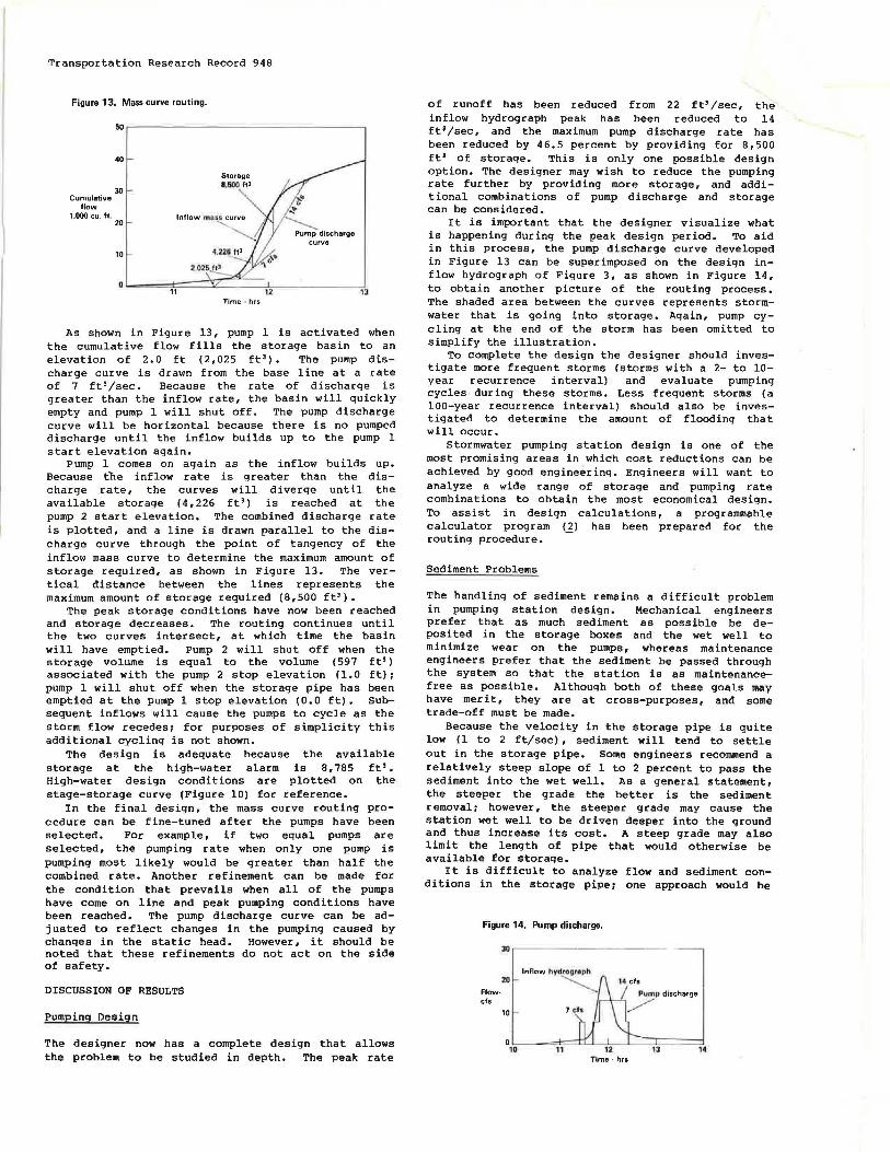
Figure 13. Mass curve routing.

40

30 Cumulative

flow 1.000 cu. ft.

20

10

Time · hrs

As shown in Figure 13, pump 1 is activated when the cumulative flow fills the storage basin to an elevation of 2,0 ft (2,025 ft'). The pump dis­charge curve is drawn from the base line at a rate of 7 ft' /sec. Because the rate of discharge is greater than the inflow rate, the basin will quickly empty and pump 1 will shut off. The pump discharge curve will be horizontal because there is no pumped discharge until the inflow builds up to the pump 1 start elevation again.

Pump 1 comes on again as the inflow builds up. Because tne inflow rate is greater than the dis­charge rate, the curves will diverge until the available storage (4,226 ft') is reached at the pump 2 start elevation. The combined discharge rate is plotted, and a line is drawn parallel to the dis­charge curve through the point of tangency of the inflow mass curve to determine the maximum amount of storage required, as shown in Figure 13. The ver­tical distance between the lines represents the maximum amount of storage required (B,500 ft').

The peak storage conditions have now been reached and storage decreases. The routing continues until the two curves intersect, at which time the basin will have emptied. Pump 2 will shut off when the storage volume is equal to the volume ( 597 ft') associated with the pump 2 stop elevation (1.0 ft); pump 1 will shut off when the storage pipe has been emptied at the pump 1 stop elevation (0,0 ft). Sub­sequent inflows will cause the pumps to cycle as the storm flow recedes; for purposes of simplicity this additional cycling is not shown.

The design is adequate because the available storage at the high-water alarm is 8,785 ft'. High-water design conditions are plotted on the stage-storage curve (Figure 10) for reference.

In the final design, the mass curve routing pro­cedure can be fine-tuned after the pumps have been selected. For example, if two equal pumps are selected, the pumping rate when only one pump is pumping most likely would be greater than half the combined rate. Another refinement can be made for the condition that prevails when all of the pumps have come on line and peak pumping conditions have been reached. The pump discharge curve can be ad­justed to reflect changes in the pumping caused by changes in the static head. However, it should be noted that these refinements do not act on the side of safety.

DISCUSSION OF RESULTS

Pumping Design

The designer now has a complete design that allows the problem to be studied in depth. The peak rate

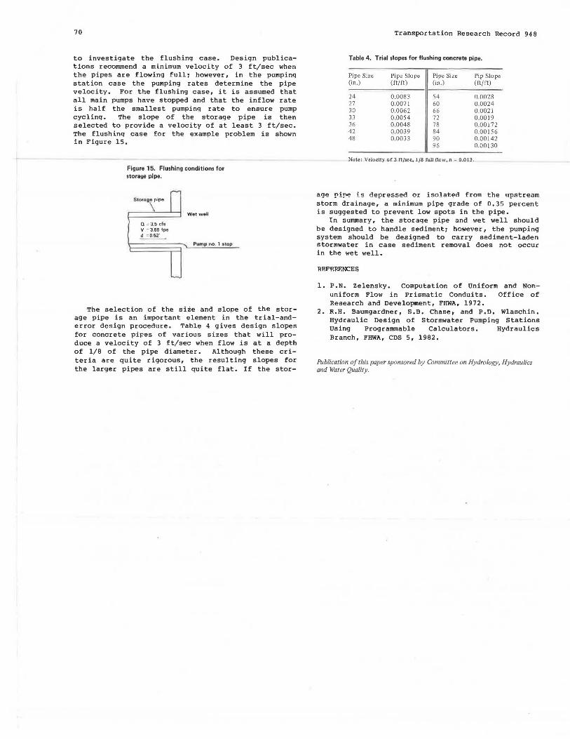
of runoff has been reduced from 22 ft' /sec, the inflow hydrograph peak has been reduced to 14 ft' /sec, and the maximum pump discharge rate has been reduced by 46.5 percent by providing for 8,500 ft' of storage. This is only one possible design option. The designer may wish to reduce the pumping rate further by providing more storage, and addi­tional combinations of pump discharge and storage can be considered,

It is important that the designer visualize what is happening during the peak design period. To aid in this process, the pump discharge curve developed in Figure 13 can be super imposed on the design in­f low hydrograph of Figure 3, as shown in Figure 14, to obtain another picture of the routing process. The shaded area between the curves represents storm­water that is going into storage, Again, pump cy­cling at the end of the storm has been omitted to simplify the illustration.

To complete the design the designer should inves­tigate more frequent storms (storms with a 2- to 10-year recurrence interval) and evaluate pumping cycles during these storms. Less frequent storms (a 100-year recurrence interval) should also be inves­tigated to determine the amount of flooding that will occur.

Stormwater pumping station design is one of the most promising areas in which cost reductions can be achieved by good engineering. Engineers will want to analyze a wide range of storage and pumping rate combinations to obtain the most economical design. To assist in design calculations, a programmable calculator program (2) has been prepared for the routtng procedure. -

Sediment Problems

The handling of sediment remains a difficult problem in pumping station design. Mechanical engineers prefer that as much sediment as possible be de­posited in the storage boxes and the wet well to minimize wear on the pumps, whereas maintenance engineers prefer that the sediment be passed through the system so that the station is as maintenance­free as possible. Although both of these goals may have merit, they are at cross-purposes, and some trade-off must be made.

Because the velocity in the storage pipe is quite low ( 1 to 2 ft/sec) , sediment will tend to settle out in the storage pipe. Some engineers recommend a relatively steep slope of 1 to 2 percent to pass the sediment into the wet well. As a general statement, the steeper the grade the better is the sediment removal; however, the steeper grade may cause the station wet well to be driven deeper into the ground and thus increase its cost. A steep grade may also limit the length of pipe that would otherwise be available for storage.

It is difficult to analyze flow and sediment con­ditions in the storage pipe; one approach would be

Figure 14. Pump discharge.

JO

ill Flow· els

10

0 10 '1 13 14

Time - hrs

70

to investigate the flushing case. Design publica­tions recommend a minimum velocity of 3 ft/sec when the pipes are flowing full: however, in the pumping station case the pumping rates determine the pipe velocity. For the flushing case, it is assumed that all main pumps have stopped and that the inflow rate is half the smallest pumping rate to ensure pump cycling. The slope of the storage pipe is then selected to provide a velocity of at least 3 ft/sec. The flushing case for the example problem is shown in Figure 15.

Figure 15. Flushing conditions for storage pipe.

Stor&gtt pipe

Q = 3.5 cfs V =J.65 fps d =O 52'

Wet well

The selection of the size and slope of the stor­age pipe is an important element in the trial-and­error design procedure. Table 4 gives design slopes for concrete piFeS of various sizes that will pro­duce a velocity of 3 ft/sec when flow is at a depth of l/B of the pipe diameter. Although these er i­ter ia are quite rigorous, the resulting slopes for the larger pipes are still quite flat. If the stor-

Transportation Research Record 948

Table 4. Trial slopes for flushing concrete pipe.

Pipe Size (in.)

24 27 30 33 36 42 48

Pipe Slope (ft/ft)

0.0083 0.0071 0.0062 0.0054 0.0048 0.0039 0.0033

Pipe Size (in .)

'i4 60 66 72 78 84 90 96

Note: Velocity of 3 ft/si;c1 l/S full flow,n = 0.013.

Pip Slope (ft/ft)

0 007.R 0.0024 0.0021 0 .0019 0.00172 0.00156 0.00142 0.00130

age pipe is depressed or isolated from the upstream storm drainage, a minimum pipe grade of 0.35 percent is suggested to prevent low spots in the pipe.

In summary, the storage pipe and wet well should be designed to handle sediment: however, the pumping system should be designed to carry sediment-laden stormwater in case sediment removal does not occur in the wet well.

RF.FF.RENCES

1. l>. N. Zelensky. Computation of Uniform and Non­uniform Flow in Prismatic Conduits. Office of Research and Development, FHWA, 1972.

2. R.H. Baumgardner, S.B. Chase, and P.D. Wlaschin. Hydraulic Design of Stormwater Pumping Stations Using Programmable Calculators. Hydraulics Branch, FHWA, CDS 5, 1982 .

Publication of this paper sponsored by Committee on Hydrology, Hydraulics and Water Quality.