human motion tracking and orientation estimation …dolev/pubs/thesis/ami-msc-thesis.pdf · human...
TRANSCRIPT

Human Motion Tracking and Orientation
Estimation using inertial sensors and
RSSI measurements
A thesis submitted in partial fulfillment
of the requirements for the degree of
Master of Science
by
Ami Luttwak
Supervised by
Prof. Danny Dolev
School of Engineering and Computer Science
The Hebrew University of Jerusalem
Israel
December 28, 2011


Acknowledgments
I wish to express my deepest gratitude to Prof. Danny Dolev. For his excellent
guidance, encouragement and great patience throughout this research. This thesis
would not have been possible without the devotion, cooperation and an endless will
to help of both Dr. Gaddi Blumrozen and Bracha Hod. I am sincerely grateful for
their help, guidance and academic cooperation. I would also like to thank to Dr.
Tal Anker for his continuous support. Finally, I wish to thank my parents for their
unmeasurable support and love.
Abstract
Real-time tracking of human body motion is an important technology in biomedical
applications, robotics, and other human computer interaction applications. Inertial
sensors can overcome problems with jitter, latency interference, line-of-sight obscura-
tions and limited range but suffer from slow drift. RSSI based location estimation can
detect location without drifting but is slow, sensitive to shadowing effects and suffers
from large estimation errors. For these reasons, most research considered RSSI-based
estimation unsuitable for Body Area Network environment. Recent work in our lab,
demonstrated an RSSI-based setup able to perform well in close proximity, rendering
it useful for human motion tracking. This paper describes the design of a complemen-
tary kalman filter to integrate the data from these two types of sensors in order to
achieve the excellent dynamic response of an inertial system without drift and with-
out the shadowing sensitivity of RSSI-based estimations. Real-time implementation
and testing results of the complementary Kalman filter are presented. Experimental
results validate the filter design, and show the feasibility of using inertial/RSSI sensor
modules for real-time human body motion tracking.

Table of Contents
Acknowledgments 3
Abstract 4
1 Introduction 14
1.1 Motivation . . . . . . . . . . . . . . . . . . . . . . . . . . . . . . . . . 15
1.2 Thesis Contribution . . . . . . . . . . . . . . . . . . . . . . . . . . . . 15
1.3 Thesis Outline . . . . . . . . . . . . . . . . . . . . . . . . . . . . . . . 16
2 Related Work 17
2.1 Inertial motion tracking . . . . . . . . . . . . . . . . . . . . . . . . . 17
2.2 Reducing drift in inertial systems . . . . . . . . . . . . . . . . . . . . 19
2.2.1 sensor fusion . . . . . . . . . . . . . . . . . . . . . . . . . . . . 19
2.2.2 Domain specific assumptions . . . . . . . . . . . . . . . . . . . 21
2.3 RSSI-based tracking . . . . . . . . . . . . . . . . . . . . . . . . . . . 22
3 System Model 24
3.1 System description . . . . . . . . . . . . . . . . . . . . . . . . . . . . 24
3.2 Inertial sensors modeling . . . . . . . . . . . . . . . . . . . . . . . . . 24
3.2.1 Rotations and Sensor co-ordinate system . . . . . . . . . . . . 25
3.2.2 The Gyroscope sensor model . . . . . . . . . . . . . . . . . . . 27
3.2.3 The Accelerometer sensor model . . . . . . . . . . . . . . . . . 28
3.3 RSSI modeling . . . . . . . . . . . . . . . . . . . . . . . . . . . . . . 28
4 Location estimation 31
4.1 Location estimation using inertial sensors . . . . . . . . . . . . . . . . 31
4.1.1 Strapdown inertial navigation . . . . . . . . . . . . . . . . . . 32

6 Table of Contents
4.1.2 Domain-specific assumptions - the orientation kalman filter . . 36
4.2 Location estimation using RSSI . . . . . . . . . . . . . . . . . . . . . 42
4.3 Location estimation using sensor fusion . . . . . . . . . . . . . . . . . 44
5 Experimental methods 55
5.1 Experiment setup . . . . . . . . . . . . . . . . . . . . . . . . . . . . . 55
5.1.1 Inertial system setup . . . . . . . . . . . . . . . . . . . . . . . 56
5.1.2 RSSI system setup . . . . . . . . . . . . . . . . . . . . . . . . 57
5.2 Comparison with optical tracking system . . . . . . . . . . . . . . . . 59
5.3 Model parameters estimation . . . . . . . . . . . . . . . . . . . . . . 59
5.4 Sensor calibration . . . . . . . . . . . . . . . . . . . . . . . . . . . . . 60
5.5 Data Synchronization . . . . . . . . . . . . . . . . . . . . . . . . . . . 64
5.6 Analysis . . . . . . . . . . . . . . . . . . . . . . . . . . . . . . . . . . 67
6 Results 68
6.1 Parameter identification . . . . . . . . . . . . . . . . . . . . . . . . . 68
6.2 Typical results . . . . . . . . . . . . . . . . . . . . . . . . . . . . . . 68
6.3 Gyroscope bias estimation . . . . . . . . . . . . . . . . . . . . . . . . 71
6.4 Accelerometer bias estimation . . . . . . . . . . . . . . . . . . . . . . 74
6.5 Sensitivity to initial condition errors . . . . . . . . . . . . . . . . . . 74
7 Discussion and Future Work 79
8 Conclusions 82
Bibliography 83

List of Figures
2.1 Comparison of position drift performance of commercial, tactical, nav-
igation, strategic-grade, and perfect pure inertial navigation systems
[1]. Note that commercial and tactical grade systems are rendered use-
less after just a few seconds. Also, even the ”perfect” ins eventually
drifts due to fluctuations in earth’s gravitational field. . . . . . . . . . 19
3.1 System description diagram. The diagram details the system’s compo-
nents , the mobile node, the anchor nodes and the control station and
the relationship between them. The mobile nodes periodically sends a
data packet to the anchor nodes, which compute the Recieved Signal
Stregnth. The control station aggregates, synchronizes and estimates
location utilizing both inertial and RSS-based estimations . . . . . . . 25
3.2 Sensor model diagram. The diagram details the components of each
signal (yG,t and yA,t) and the relationships between them. Gyroscope
signal is modeled as the angular velocity component ωt, a white noise
component vG and a slowly varying gyroscope bias wbg. The orienta-
tion GSR is computed from the gyroscope signal using the box ’inte-
gration’. The acceleration signal yA,t is composed of the acceleration
and gravity vector relative to the sensor’s frame (Sa −S g), a white
measurement noise vA . . . . . . . . . . . . . . . . . . . . . . . . . . 26
8 LIST OF FIGURES
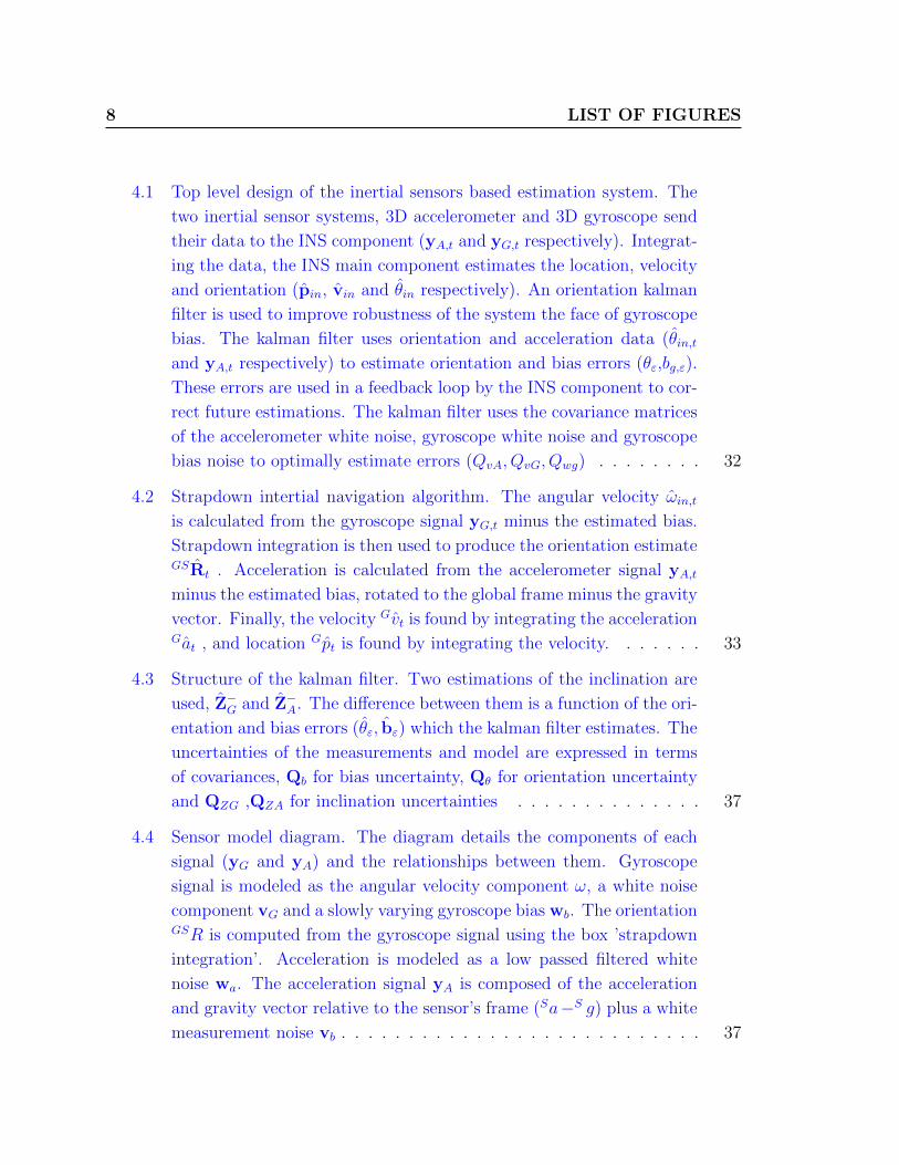
4.1 Top level design of the inertial sensors based estimation system. The
two inertial sensor systems, 3D accelerometer and 3D gyroscope send
their data to the INS component (yA,t and yG,t respectively). Integrat-
ing the data, the INS main component estimates the location, velocity
and orientation (pin, vin and θin respectively). An orientation kalman
filter is used to improve robustness of the system the face of gyroscope
bias. The kalman filter uses orientation and acceleration data (θin,tand yA,t respectively) to estimate orientation and bias errors (θε,bg,ε).
These errors are used in a feedback loop by the INS component to cor-
rect future estimations. The kalman filter uses the covariance matrices
of the accelerometer white noise, gyroscope white noise and gyroscope
bias noise to optimally estimate errors (QvA, QvG, Qwg) . . . . . . . . 32
4.2 Strapdown intertial navigation algorithm. The angular velocity ωin,tis calculated from the gyroscope signal yG,t minus the estimated bias.
Strapdown integration is then used to produce the orientation estimateGSRt . Acceleration is calculated from the accelerometer signal yA,tminus the estimated bias, rotated to the global frame minus the gravity
vector. Finally, the velocity Gvt is found by integrating the accelerationGat , and location Gpt is found by integrating the velocity. . . . . . . 33
4.3 Structure of the kalman filter. Two estimations of the inclination are
used, Z−G and Z−A. The difference between them is a function of the ori-
entation and bias errors (θε, bε) which the kalman filter estimates. The
uncertainties of the measurements and model are expressed in terms
of covariances, Qb for bias uncertainty, Qθ for orientation uncertainty
and QZG ,QZA for inclination uncertainties . . . . . . . . . . . . . . 37
4.4 Sensor model diagram. The diagram details the components of each
signal (yG and yA) and the relationships between them. Gyroscope
signal is modeled as the angular velocity component ω, a white noise
component vG and a slowly varying gyroscope bias wb. The orientationGSR is computed from the gyroscope signal using the box ’strapdown
integration’. Acceleration is modeled as a low passed filtered white
noise wa. The acceleration signal yA is composed of the acceleration
and gravity vector relative to the sensor’s frame (Sa−S g) plus a white
measurement noise vb . . . . . . . . . . . . . . . . . . . . . . . . . . . 37

LIST OF FIGURES 9
4.5 Inclination estimation process. The angular velocity ω−t is calculated
from the gyroscope signal yG,t minus the estimated bias. Strapdown
integration is then used to produce the orientation estimate GSR−t and
inclination GSZ−G,t. Acceleration Ga−G,t is calculated from the previ-
ous estimation multiplied by a factor, and then rotated to the sensor
frame. Finally, the inclination estimation SZ−A,t is calculated from the
accelerometer signal and accelerometer estimation using 4.11 . . . . . 39
4.6 Selecting the intersection point closest to the object location . . . . . 44
4.7 Top level design of the system. The system is composed of two in-
dependent sub systems that estimate the location, the kalman filter
estimates the errors and corrects them using a feedback loop. Two
estimations of the location are used, p−INS and p−RSSI . The difference
between them is a function of the location,velocity, orientation and
bias errors (pε, vε, θε, ba,ε, bg,ε) which the kalman filter estimates. The
uncertainties of the measurements and model are expressed in terms
of covariances, Qwa and Qwg for bias uncertainties, QvA and QvG for
sensor white noise ,QvR for RSSI estimation uncertainties and Qwr for
RSSI shadowing uncertainties . . . . . . . . . . . . . . . . . . . . . . 45
5.1 Experiment setup. Tracking of the hand movement across the 2D sur-
face is accomplished by attaching several sensors to the moving hand.
For inertial movement information, the SHIMMER sensor is used. For
location estimation using RSSI, two BSN nodes are used as anchor
nodes and one BSN node is attached to the hand. The system results
are compared to reference information provided by the optical tracking
system Polaris. The Polaris system uses a passive marker mounted on
the moving hand. . . . . . . . . . . . . . . . . . . . . . . . . . . . . 56

10 LIST OF FIGURES
5.2 Block diagram of the experiment data flow. Sensor data from the
SHIMMER and BSN node is calibrated and pre-processed. All data
sources are synchronized, and a uniform time stamp is determined. The
location estimation process is composed of the INS and RSSI location
estimations (p−INS and p−RSSI respectively). The kalman filter uses both
estimations to predict the errors pε. The INS errors are corrected in a
feedback loop and the location estimation is computed p+INS. Polaris
location estimation ppolaris is then compared to results and the Mean
Squared Error is calculated. . . . . . . . . . . . . . . . . . . . . . . . 57
5.3 The mobile node attached to the hand. A SHIMMER sensor is used
for capturing INS information, a BSN node transmits data packets for
RSSI measurements and a Polaris passive marker is used by the Polaris
system to track the moving hand . . . . . . . . . . . . . . . . . . . . 58
5.4 The SHIMMER wearable sensor platform. SHIMMER incorporates
a TI MSP430 processor, a CC2420 IEEE 802.15.4 radio, a triaxial
accelerometer, and a rechargeable Li-polymer battery. A triaxial gy-
roscope board is added as an internal expansion with two dual-axis
gyroscope chips. The platform also includes a MicroSD slot support-
ing up to 2 GB of Flash memory . . . . . . . . . . . . . . . . . . . . 58
5.5 The polaris tracking setup. Two passive markers are used. The first is a
static marker, placed in the origin of axis defined by the RSSI tracking
system. The second is a mobile marker attached to the moving hand. 59
5.6 Transfer function of the accelerometer sensor. S is the slope of the
transfer function.VOFF is the offset error. . . . . . . . . . . . . . . . . 60
5.7 Calibration sequence. The Shimmer is placed on a different face ev-
ery few seconds. (a) 3-axis accelerometer sensor recording of the cal-
ibration process. The earth-facing(sky-facing) sensor is automatically
detected for each position, and the average value is computed, corre-
sponding to g(−g).(b) 3-axis gyroscope sensor recording of the calibra-
tion process. A moving average method was used to detect the turns
along each axis. Integrating the signal input over the complete turn
corresponds to a 90 degrees turn value. . . . . . . . . . . . . . . . . . 62

LIST OF FIGURES 11
5.8 Validation sequence. The sensor placed in a different static 3-D po-
sition every few seconds. The magnitude of the acceleration vector is
expected to be the gravity force g. (a) The 3-axis accelerometer output
and the calculated norm. (b) Comparison of the magnitude to the ex-
pected gravity. In the example there are fluctuations of 0.5m/s2 which
might cause considerable errors. . . . . . . . . . . . . . . . . . . . . . 63
5.9 Shimmer and BSN mobile node synchronization. Shimmer accelerom-
eter and BSN accelerometer signals are shown after synchronization.
Even though the BSN signal is not properly calibrated, the sync oper-
ation performs well. . . . . . . . . . . . . . . . . . . . . . . . . . . . . 65
5.10 Shimmer and Polaris system synchronization. Shimmer gyroscope and
Polaris computed gyroscope signals are shown after synchronization.
The polaris gyroscope signal is very noisy due to the derivation process,
yet the sync operation works well. The shimmer gyroscope suffers from
changing bias, most evident in the first 10 seconds. . . . . . . . . . . 66
6.1 Measured sensor signals during one hand movement experiment (2D
movement). (a) Accelerometer output vector, only x,y axis are shown
since movement is 2D. (b) Gyroscope output vector. The gyroscope
changing bias can be seen in the first 10 seconds before the hand starts
moving. . . . . . . . . . . . . . . . . . . . . . . . . . . . . . . . . . . 69
6.2 RSSI location error. The graph shows a changing bias with time con-
stant of about 5 seconds. This constant is used to model the RSSI
error. . . . . . . . . . . . . . . . . . . . . . . . . . . . . . . . . . . . 70
6.3 Typical results for location estimations. Each plot shows the kalman-
based,RSSI-based and reference estimations. Inertial-based estimation
diverges quickly and is not presented. . . . . . . . . . . . . . . . . . . 71
6.4 Typical results for location and location estimation error (LEE) de-
composed for X and Y axis. Plot (a) compares the location estimation
of the proposed filter with the RSSI-based estimation. The kalman
filter tracks the movement and shape much better but overall RMS
sense is quite similar as shown in plot (b). . . . . . . . . . . . . . . . 72
6.5 Trace of the kalman gain matrix. The graph shows that the gain con-
verges after 10 seconds. . . . . . . . . . . . . . . . . . . . . . . . . . . 73

12 LIST OF FIGURES
6.6 Filter tracking of gyroscope bias drift. Plot (a) compares the estimated
Gyroscope bias with the actual changing bias. Plot (b) shows the Bias
Estimation Error as a function of time. . . . . . . . . . . . . . . . . 74
6.7 Comparison of filter performance compared to simpler model without
gyroscope bias model. The top plot shows the Location Estimation
Error of X axis(LEEx) for the two filters. The LEE. The LEEx for the
simple model grows due to growing error in the orientation estimation
(OOE) as shown in the lower plot. The plots clearly demonstrate that
the simpler model performance is inferior in face of constant Gyroscope
bias . . . . . . . . . . . . . . . . . . . . . . . . . . . . . . . . . . . . 75
6.8 Gyroscope bias tracking during an experiment starting from a static
position. The bias cannot be determined during the initial static pe-
riod, it is corrected only on the 8th second when movement starts.
Note the velocity trace is plotted only for reference of movement time,
y-axis units are not relevant. . . . . . . . . . . . . . . . . . . . . . . . 76
6.9 Comparison of filter tracking changing bias for different values of Qwg
[defined in 3.7]. Setting a small value, causes slow divergence . . . . 76
6.10 Accelerometer bias tracking. Estimated accelerometer bias values are
plotted compared to the real values. The filter converges to the correct
bias values for both X and Y axis. . . . . . . . . . . . . . . . . . . . . 77
6.11 Location estimation for the X axis with wrong initial conditions. The
plots show wrong initial X values of 0.5 M, 1 M and 1.5 M. The different
traces show the filter converges after at most 20 seconds even for large
errors. . . . . . . . . . . . . . . . . . . . . . . . . . . . . . . . . . . . 77
6.12 Velocity estimation for the X axis with wrong initial conditions. The
plots show wrong initial X values of 1 M/S, 2 M/S, -1 M/S and -2 M/S.
The different traces show the filter converges after at most 25 seconds
even for large errors. . . . . . . . . . . . . . . . . . . . . . . . . . . . 78
6.13 Orientation estimation error. Orientation is represented as a counter
clock-wise rotation in the XY plane. The plots show wrong initial
values of 1 RAD, 2 RAD, -1 RAD and -2 RAD. For large errors, the
convergence occurs only after considerable time. . . . . . . . . . . . . 78

List of Tables
6.1 Kalman filter initialization parameters. . . . . . . . . . . . . . . . . . 70
6.2 RMSE values for each estimation method. The kalman filter achieves
greater accuracy, improving the RSSI estimates by 10-20% . . . . . . 72
6.3 RMSE values for each Qwg value for a typical experiment with little
bias. Filter performance is affected if an inappropriate value is used. . 73
7.1 RMSE values for each estimation method from simulation results . . 81
Chapter 1
Introduction
Recent advances in electrical, biological, chemical and mechanical sensor technologies
have led to a wide range of wearable sensors suitable for long autonomous opera-
tion and continuous monitoring [2]. Using small wearable wireless platforms that can
record and transmit physiological and kinematic data in real-time, human movement
can now be measured continuously outside a specialized laboratory [3]. Applications
in many medical fields such as gait analysis ([4],[5],[6]), functional electrical stimula-
tion ([7], [8], [9]) and monitoring activities of daily living (ADL) ([10],[11], [12]). Thus,
research is currently being carried out in many laboratories for designing systems for
better and accurate tracking of human body motion with the use of on-board MEMS
sensors. Beside the research efforts for high-grade, yet inexpensive sensors, advanced
signal processing methods are intensely investigated to improve the performance of
tracking algorithms [13].
Calculating orientation and location using these miniaturized inertial systems
has limited capabilities. The main problem is that location is computed by time-
integrating the signals from gyros and accelerometers, including any superimposed
sensor drift and noise. Hence, the estimation errors tend to grow unbounded.[refs]
Solutions for mitigating the drift problem usually consist of an external sensors such
as magnometers [14] or on problem-specific knowledge, for example gait cycle for drift
error correction [15].
This paper presents a new design for mitigating the drift errors by integrating RSSI
data into the estimation process. The main benefit of employing RSSI information is
that it comes with no added hardware costs as all existing wireless sensor platforms
support it. However, since RSSI estimation in these ranges is greatly affected by
multi-path phenomenon, advanced signal processing methods must be used. We
1.1 Motivation 15
present a complementary kalman filter model designed to optimally fuse the inertial
sensors data and the RSSI data. The basic idea behind complementary filtering
is that location and orientation drift errors resulting from accelerometer and gyro
output errors can be bounded by aiding the estimation with additional sensor data,
the information from which allows correcting the inertial sensors solution. Body
segment location estimation obtained with this system was compared with a location
estimation obtained using a laboratory bound camera system.
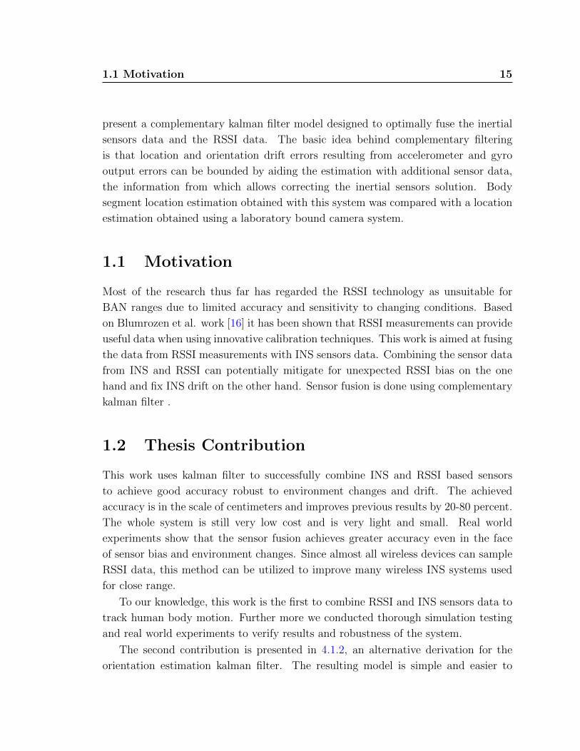
1.1 Motivation
Most of the research thus far has regarded the RSSI technology as unsuitable for
BAN ranges due to limited accuracy and sensitivity to changing conditions. Based
on Blumrozen et al. work [16] it has been shown that RSSI measurements can provide
useful data when using innovative calibration techniques. This work is aimed at fusing
the data from RSSI measurements with INS sensors data. Combining the sensor data
from INS and RSSI can potentially mitigate for unexpected RSSI bias on the one
hand and fix INS drift on the other hand. Sensor fusion is done using complementary
kalman filter .
1.2 Thesis Contribution
This work uses kalman filter to successfully combine INS and RSSI based sensors
to achieve good accuracy robust to environment changes and drift. The achieved
accuracy is in the scale of centimeters and improves previous results by 20-80 percent.
The whole system is still very low cost and is very light and small. Real world
experiments show that the sensor fusion achieves greater accuracy even in the face
of sensor bias and environment changes. Since almost all wireless devices can sample
RSSI data, this method can be utilized to improve many wireless INS systems used
for close range.
To our knowledge, this work is the first to combine RSSI and INS sensors data to
track human body motion. Further more we conducted thorough simulation testing
and real world experiments to verify results and robustness of the system.
The second contribution is presented in 4.1.2, an alternative derivation for the
orientation estimation kalman filter. The resulting model is simple and easier to

16 Introduction
implement.
1.3 Thesis Outline
The thesis is organized as the following.
Chapter 2 introduces the related work that was done in this area. The system
model is presented in Chapter 3. Chapter 4 presents the problem formally and de-
scribes the solution
Chapter 5 deals with the experimental methods and setup. The experiments
results and analysis are provided in chapter 6. Chapter 7 provides a through discussion
of the results and future work. Finally, Chapter 8 summarizes the presented work
and outlines the conclusions.

Chapter 2
Related Work
In recent years, technological advancements have made it possible to record human
movement continuously outside the boundaries of the laboratory [17]. Wearable wrist-
size sensor platform that can record inertial movement are now commercially avail-
able. The SHIMMER [3] and XSENS [18] platforms are small wireless sensor plat-
forms that can record and transmit physiological and kinematic data in real-time and
are widely used for medical research. The UP wristband by Jawbone [19] is a wireless
wristband aimed for the general public, collecting every day life statistics such as
sleep time and steps count. As these technologies are now widespread, the topic of
human motion tracking and gait analysis is of great interest in everyday applications
generating a large amount of research into systems that can provide this information
in real time at a low-cost and with the smallest intrusion level possible [20].
2.1 Inertial motion tracking
Inertial navigation systems (INSs) were widely used for ships, submarines, and air-
planes starting from the 1950s [21]. Over the course of the last 20 years, developments
in fields of electronics and micromachining, pushed by the needs of the automotive
and consumer industry have produced low-cost, small sized silicon sensors leading to
new applications [17]. Inertial sensors have been extensively used in the automotive
industry [22], robotics [23] and augmented reality [24]. In recent years, they have also
applied into the implementation of human motion tracking [20].
Inertial trackers are of prime importance in human motion tracking. They have
fewer costs, compact size, lightweight, and no motion constraint. They are com-
pletely self-contained, so they have no Line Of Sight (LOS) requirements, no emitters

18 Related Work
to install, and no sensitivity to interfering electromagnetic fields or multipath effects.
Also, they have very low latency and can be measured at relatively high rates (thou-
sands of samples per second) [25]. Sadly, they have a major drawback that is hard
to overcome, the drift problem. There are several causes of drift in a system which
obtains orientation by integrating the outputs of angular rate gyros [26]:
• Constant bias δω - when integrated causes a steadily growing angular error
θtδω · t
• Thermo-Mechanical White Noise vt - when integrated leads to a random walk
process θt =∫ t
0vtdt which has an expected value zero but a mean squared error
growing linearly with time.
• Calibration errors in the scale factors, alignments, and linearities of the sensors,
produce measurement errors leading to the accumulation of additional drift.
• Flicker Noise / Bias Stability - during operation the bias wanders away, pro-
ducing a residual bias that gets integrated to create second-order random walk.
Bias stability is usually modeled as a random walk or Gauss-Markov process,
and is often the critical parameter for drift performance, since constant bias can
usually be calibrated and compensated effectively.
For position estimation the drift problem is even more severe. First, there are ac-
celerometer errors corresponding to the 4 gyro errors listed above. However, since
the position is obtained by double integrating acceleration, a fixed accelerometer bias
error results in a position drift error that grows quadratically in time. But the critical
cause of error in position measurement is error in the orientation estimation. An error
of δθ in tilt angle will result in an error of g · sin(δθ) in the horizontal components of
the acceleration . For this reason, in practice, it is the gyroscopes, not the accelerom-
eters which limit the positional navigation accuracy of most INS systems. As seen
in fig 2.1, the simulation shows that commercial-grade inertial navigation systems
suffer from large position drift after just a few seconds [1]. Therefore, exploring new
techniques to reduce drift in inertial systems is a primary goal in the field of human
motion tracking.

2.2 Reducing drift in inertial systems 19
Figure 2.1: Comparison of position drift performance of commercial, tactical, nav-igation, strategic-grade, and perfect pure inertial navigation systems [1]. Note thatcommercial and tactical grade systems are rendered useless after just a few seconds.Also, even the ”perfect” ins eventually drifts due to fluctuations in earth’s gravita-tional field.
2.2 Reducing drift in inertial systems
Many studies of reducing drift in inertial systems for human motion tracking have
been performed. Different systems with varying number, type and configuration of
sensors used, some studies are limited to tracking two degrees of orientation in a
plane, while others track 3-D orientation [27]. Algorithms have also been designed
to track limb segment orientations relative to each other or calculate joint angles
[28]. Generally, the solutions for the drift reduction problem fall into one of the two
categories, sensor fusion and the application of domain specific assumptions.
2.2.1 sensor fusion
Sensor fusion is the process of combining sensory data from two or more types of sen-
sors to update the state of a system. In inertial systems, the state usually consists of

20 Related Work
position, velocity and orientation of the object. A sensor fusion algorithm calculates
the state using inertial sensors signals together with signals from additional sources
such as magnetometers [29]. Several mathematical and statistical tools are employed
in current research to fuse sensor data for tracking. The most prominent methods
are particle filter and various variants of the kalman filter ,mainly EKF, unsentenced
kalman and complementary kalman filter. Many types of complementing sensor tech-
nologies are found in the literature, among them optical [30], Ultra Wide Band [31],
GPS [32], magnetometer [28], and acoustical sensors [33].
The integration of visual and inertial sensors for human motion tracking has re-
ceived much attention lately, due to its robust performance and wide potential ap-
plication [34]. Most systems use an extended kalman filter for sensor fusion. The
most popular representant is the commercially available InterSense VIS-Tracker [35].
In [30] a real-time hybrid solution is presented to articulated 3D arm motion track-
ing for home-based rehabilitation by combining visual and inertial sensors. Data
fusion is also done using Extended Kalman Filter.In [36] the FlightTracker system
was presented to track a pilot’s head movement. They developed a differential inertial
measurement equation of the pilots head motion relative to the aircraft, which can
then have its drift corrected by periodic optical measurements of the head position
relative to the aircraft. Inertial sensors can provide cues about the observed scene
structure. This information can be used to simplify 3D reconstruction of the observed
world. Lobo and Dias [37] use inertial sensors to find a vertical reference and use it
to determine the image horizon line. Similar work has been described in these refs
[38],[39].
Another type of sensor commonly used to reduce drift is the vector magnetometer.
The magnetometers measure the strength and direction of the local magnetic field,
allowing the north direction to be found. Magnetometers are susceptible to interfer-
ence of ferromagnetic materials which distort the orientation measurement, therefor
they are not accurate enough to replace gyroscopes [ref]. However, they can be used
efficiently together with gyroscope data to improve the accuracy of the calculated
orientation. Foxlin [40] and Bachman [28] presented filters in which accelerometers
and magnetometers are used for low frequency components of the orientation and
gyroscopes to measure faster changes in orientation. In [29] a complementary kalman
filter was designed to overcome ferromagnetic disturbances by calculating a magnetic
disturbance vector. The main advantage of this approach is that the tracking system
remains self contained. The main disadvantage is that it only reduces the drift growth

2.2 Reducing drift in inertial systems 21
rate, rather than allowing absolute corrections to be applied.
2.2.2 Domain specific assumptions
In some applications, assumptions of the movement of the body can be made and
used to reduce drift. One of the best examples for using domain specific assumptions
is NavShoe [41] where a shoe mounted IMU is used for pedestrian tracking.When a
person walks, their feet alternate between a stationary stance phase and a moving
stride phase. The system uses the stance phase for zero velocity updates, allowing
drift in velocity to be corrected. By measuring the acceleration due to gravity during
the stationary phase, inclination errors can also be corrected. The work of Yun [42]
also uses the periodic nature of walking for precise drift error correction. In [43],
Luinge presented a complementary kalman filter for human body segment orientation
fusing gyroscope and accelerometer data. The system models the characteristic ac-
celeration of body segments as a first order low-pass filtered white noise process. In
similar work, Bachman [44] present a quaternoin based kalman filter for inertial track-
ing. The filter continuously corrects the drift based on the assumption that human
limb acceleration is bounded, and averages to zero over any extended period of time.
Another approach for domain specific assumptions is the use of kinematic constraints
model.Young [45] demonstrated a method for estimating the linear acceleration of
IMUs based on subject body model constraints. Zhou and Hu [46] developed a kine-
matic model for human upper limb movement which helps at removing undesirable
biases or noise. Using this model, they construct a kalman filter which fuses inertial
sensors data to track human movement.
The work in this research employs both techniques for drift reduction. First,
domain specific assumption is employed in the orientation estimation. The limb
acceleration is assumed to be small compared to the gravity which allows the filter to
continuously obtain an inclination estimate using the signal of the 3D acceleromter.
This estimate is then used by a complementary kalman filter to continuously reduce
the gyroscope drift [43]. Second, sensor fusion is employed to optimally combine the
inertial system estimations with RSSI-based position estimations. The sensor fusion
is also implemented using a complementary kalman filter.

22 Related Work
2.3 RSSI-based tracking
RSSI-based tracking systems are mainly used in the context of indoor localization.
In general, indoor localization algorithms are aimed at locating wirelessly an object
or a person inside a building [47]. They assume the presence of a limited number of
reference nodes, referred to as anchor nodes, which know their own coordinates and
are used as reference points for localizing the other nodes [48]. RSSI-based tracking
systems use Received Signal Strength Indication (RSSI) to get an estimate of the
distance between transmitter and receiver (ranging) [49]. Sadly, the indoor radio
channel is very unpredictable, since reflections of the signal from furniture, walls,
floor and ceiling may result in severe multipath interference at the receiving antenna.
This results in range estimation errors which translate to large positioning errors [50].
Nonetheless, RSSI-based algorithm are intensively studied for indoor tracking due to
many advantages over other physical layer measurements such as acoustic Time Of
Arrival systems [51]. Compared to other solutions, pure RSSI methods are low cost,
low energy and can be easily deployed in wireless sensor network platforms, since
RSSI data is natively supported by most of the existing transceiver chipsets, with no
extra hardware costs [48].
RSSI-based localization algorithms are mostly in one of two categories, range-
based and range-free algorithms. Range-based algorithms use the RSSI signal to
estimate the distance between nodes. Then, the object position is estimated using
several techniques such as triangulation and trilateration [52],[53]. This method is
susceptible to multipath and shadowing effects and thus has limited accuracy. Range-
free algorithms do not use the RSSI value to compute distance, but exploit it in
other ways. In RSSI mapping technique, the RSSI value is interpreted using a pre-
calculated RSSI map. Systems such as RADAR [54] require a preliminary accurate
mapping of RSSI values in each position on the map. Comparing the RSSI values
received from the different anchors with the pre-built RSSI map, a node can estimate
its own position in the area.
RSSI-based tracking systems accuracy is in the scale of a meter [55].Therefor RSSI
was not considered a viable solution for the human motion tracking problem which
requires a much better accuracy. In recent work, Blumrozen et al. [56] suggested that
under certain condition, RSSI can be a valid solution for the human motion tracking
problem. Using anchor nodes in close proximity, transmitting in high frequencies,
the RSSI-mapping based system achieved accuracy of several centimeters. In [16],

2.3 RSSI-based tracking 23
the work is extended with a more elaborate calibration scheme, advanced processing
techniques and additional real life experiments. Since RSSI is readily deployable
with no extra hardware needed, it is a prime candidate to be used in sensor fusion
with an inertial system. This research uses a complementary kalman filter to fuse
the described RSSI system with inertial system’s data to solve the human tracking
problem.
Fusing RSSI and inertial sensors’ data has been previously done only in the context
of indoor localization. In [57] Klingbeil presents a modular framework for fusion of
many types of sensory input, among then RSSI and inertial tracking. The sensor
fusion is done using particle filter. In [58] Fink presents an RSSI-based system which
uses diversity and sensor fusion of RSSI and inertial sensors to achieve must better
precision. The diversity concept is using RSSI with redundant data transmission in
different frequency bands which can reduce the dropout probability. In another work,
Evennou et al. [59] presents a system for pedestrian localizations by means of sensor
fusion of WiFi signal strength measurments with inertial sensors signals. A structure
based on a Kalman filter and a particle filter is proposed.

Chapter 3
System Model
3.1 System description
The system components are illustrated in Figure 3.1. The system consists of a single
mobile node and N static nodes, referred to as anchor nodes. Each node is equipped
with wireless transceiver that can periodically transmit data. The mobile node trans-
mits a data packet with a known transmission power to the anchor nodes. The anchor
nodes, located in the transmission range of the mobile node, calculate the received
power values (RSSI). The mobile node is also equipped with inertial sensors (minia-
ture gyroscope and accelerometer) which record the node’s inertial data. The goal
of this work is to continuously estimate the mobile node’s location from the mobile
node inertial data and from the attenuation of the electromagnetic signal in space as
measured by the anchor nodes.
The research is aimed at solving the location estimation problem in the realm
of human body movement. Hence, the mobile node is assumed to be attached to a
human body part. This restriction is used to design a solution tailored for the BAN
environment, greatly improving results.
3.2 Inertial sensors modeling
The system is composed of a 3D accelerometer sensor and a 3D gyroscope sensor.
Other types of sensors, such as magnetic compass, can be possibly combined and
used in the future to further improve results [28]. Figure 3.2 depicts the inertial
sensors model as described in detail in the following sections.

3.2 Inertial sensors modeling 25
Mobile node
Anchor node
Anchor node Anchor node
Anchor node
Anchor node Anchor node
Control station
Figure 3.1: System description diagram. The diagram details the system’s compo-nents , the mobile node, the anchor nodes and the control station and the relation-ship between them. The mobile nodes periodically sends a data packet to the anchornodes, which compute the Recieved Signal Stregnth. The control station aggregates,synchronizes and estimates location utilizing both inertial and RSS-based estimations
3.2.1 Rotations and Sensor co-ordinate system
Let us denote the location, velocity and acceleration of the object c in the global
co-ordinate system by G~pc,G~vc,
G~ac , respectively. The superscripts G and S are used
to denote vectors that are expressed in the global and sensor co-ordinate systems,
respectively, i.e. S~ac is the object’s acceleration in the sensor frame.
The orientation of the sensor with respect to the global co-ordinate system is
expressed with a rotation matrix containing the three unit vectors of the global co-
ordinate system expressed in the sensor frame [43].
GSR =[SX SY SZ
]T. (3.1)

26 System Model
𝑎𝑡 𝐺 − 𝑔𝑡
𝐺
𝑅𝑡 𝐺𝑆
𝑤𝑏𝑎
−
𝑔𝑡 𝐺
𝑎𝑡 𝐺
𝜔𝑡
𝑦𝐺,𝑡 𝑤𝑏𝑔 bias
rotate
𝑣𝐺
bias
𝑣𝐺
𝑦𝐴,𝑡
𝑅 𝐺𝑆
𝑖𝑛𝑖𝑡
Integration
Figure 3.2: Sensor model diagram. The diagram details the components of each signal(yG,t and yA,t) and the relationships between them. Gyroscope signal is modeled asthe angular velocity component ωt, a white noise component vG and a slowly varyinggyroscope bias wbg. The orientation GSR is computed from the gyroscope signal usingthe box ’integration’. The acceleration signal yA,t is composed of the acceleration andgravity vector relative to the sensor’s frame (Sa−S g), a white measurement noise vA
and a slowly varying accelerometer bias wba.
The rotation matrix is a linear transformation to the global co-ordinate system
G~ac =GS R · S~ac.
Transformations can also be expressed in terms of rotation vector ~θ. The rotation is
expressed as a single rotation along the axis of the vector.
~θ = θ · e.
Where e = [eX eY eZ ]T is a three dimensional unit vector representing the axis
of turn and θ is a scalar representing the angle of rotation. This representation is
very useful since it expresses a rotation in only 3 scalars, thus simplifying the kalman
state. Another useful property is that gyroscope sensor readings are easily expressed
in this form. If T is the time sample, and ωt is the angular velocity, the rotation

3.2 Inertial sensors modeling 27
can be represented as a rotation vector Tωt . Further more, for small rotations, the
relationship between the original vector and the rotated vector is given by [60]
Gv =S v(I +
[GSθ×
]). (3.2)
Where GSθ× is a small rotation vector from S to G. This equation also applies to
the orientation matrices, yielding the following property
newR =old R (I + [θ×]) . (3.3)
3.2.2 The Gyroscope sensor model
The gyroscope signal is modeled [61] as a combination of white measurement noise
vG,t, gyroscope bias bt and the angular velocity ωt
yG,t = ωt + bgt + vG,t. (3.4)
Where vG,t is a white noise process with covariance QvG [43].
vG,t ∼ N(0, σ2
g,t
)(3.5)
The gyroscope bias is modeled as a slowly varying signal [62]. The bias fluctuations
are caused by changing properties of the sensor (such as temperature, mechanical wear
and battery power level). The model is a first order Markov process, driven by a small
white Gaussian noise.
bg,t = bg,t−1 + ∆twbg,t. (3.6)
Where ∆T is the time step and wbg,t is a white noise process with covariance Qwg.
wb,t ∼ N(0, σ2
wg,t
)(3.7)
The equivalent formula in the continuous mode yields
bg,t = wbg,t. (3.8)
Where b is the derivative of b.

28 System Model
3.2.3 The Accelerometer sensor model
The accelerometer signal is modeled as the sum of the acceleration vector S~at,the
gravity vector, small sensor bias ba,t and white gaussian measurement noise vA,t [43].
All vectors are in the sensor’s reference frame.
yA,t =S at −S gt + ba,t + ∆tvA,t. (3.9)
Where vA,t is a white noise process with covariance QvA.
vA,t ∼ N(0, σ2
A,t
)(3.10)
The accelerometer bias is modeled similarly to the gyroscope bias model [62]
ba,t = ba,t−1 + ∆twba,t. (3.11)
Where T is the time step and wba,t is a white noise process with covariance Qwa.
wba,t ∼ N(0, σ2
wa,t
)(3.12)
The equivalent formula in the continuous mode yields
ba,t = wba,t. (3.13)
3.3 RSSI modeling
Received Signal Strength Indicator (denoted RSSI) is an indication of the power level
received by the antenna. In the context of this research, RSSI measurements are
performed between the mobile node and several anchor nodes (see Section 3.1). The
antennas are assumed to be omnidirectional. The RSSI signal is affected by the
changing properties of the signal dispersion due to reflections and other multi path
phenomenon. The received signal power at the anchor node is given by the formula
[63]
Lrti = Lt+ A− q10 log10 dti + αt. (3.14)
Where Lt is the transmission power, Lrti is the received signal power at node i, dti is
the distance between the anchor node i and the mobile node, A is a constant power

3.3 RSSI modeling 29
offset which is determined by several factors, like receiver and transmitter antenna
gains and transmitter wave length , q is the channel exponent which varies between
2 (free space) and 4 (indoor with many scatterers), and αt is a Gaussian distributed
random variable with zero mean and standard deviation σα that accounts for the
random effect of shadowing. Note that αt may be correlated between successive
measurements, due to temporal shadowing phenomenon.
Combining RSSI data from several anchor nodes, allows for exact location esti-
mation pt using triangulation or similar methods (see [16]).
pt = f
([Lrti
]Ni=1
).
The RSSI based location estimation pt is affected by the changing properties of
the signal dispersion due to reflections and other multi path phenomenon. It can be
modeled as a sum of the actual position, slowly varying shadowing factor, and an
instantaneous white Gaussian noise:
pt = pt + br,t + vR,t. (3.15)
Where pt is the real location, br,t is the bias error and vR,t is a simple white noise
process with covariance QvR.
vR,t ∼ N(0, σ2
r,t
)(3.16)
The bias br,t is related to shadowing phenomenon and to directionality of the
antenna. The bias is correlated between successive measurements, due to large scale
fading factor in the αt component from the Formula 3.14. The correlation caused by
deflections from objects can be modeled as a first order Gauss-Markov process [64]
with auto correlation function of
Rbr (t) = E (br,t′ ,br,t′+t) = σ2bre− |t|τ .
Where σ2br is the variance and τ is the correlation time of the interference that could
be due to a reflecting object and other multi path phenomenon. Notice that the corre-
lation time τ is dependent of the movement speed and path properties. Experiments
data shows that τ should be in the range of 0.5-1 seconds for most human motion
scenarios.
The Gauss-Markov process can be represented in state space representation ([65],[61])

30 System Model
as follows
br,t = e−|∆t|τ br,t−1 + ∆twr,t. (3.17)
Where τ is the time constant, ∆t is the discrete time step and wr,t white noise process
with the covariance Qwr
wr,t ∼ N(0, σ2
br,t
)(3.18)
For continuous time systems, the following formula is used [66]
brt = −1
τbrt +
√2σ2u (t) .
The state space representation of the noise model is of significant importance
since kalman filter inputs must be in that form. More specifically, kalman filter can
be extended to work with colored noise, only if the noise can be represented in the
state space representation [67].
Chapter 4
Location estimation
This chapter explores the problem of optimal location estimation. Section 4.1 solves
the estimation problem when only inertial data is used. Then , section 4.2 solves the
estimation problem when only RSSI data is available. Finally, section 4.3 presents a
solution for estimating location using both data sources using advanced sensor fusion
methods. The sensor fusion is accomplished using a complementary kalman filter,
constantly estimating errors and sending feedback to the INS system.
4.1 Location estimation using inertial sensorsThis section explores the problem of optimally estimating location using inertial sen-
sors data only. The IMU (Inertial Measurement Unit) is composed of 3D accelerom-
eter and gyroscope systems which are strapped to a human body part, constantly
recording the movement as presented in Section 3.1.
The system design is depicted in Figure 4.1. Section 4.1.1 details the operation of
the basic INS component, which integrates the sensors’ data to compute a location
estimate. As previously explained in Section 2.1, INS systems suffer greatly from
integration drift and sensor bias. These error factors are so acute that they render
the estimation useless after a short time. Section 4.1.2 derives a kalman filter for
orientation estimation that can improve the inertial system’s results. It uses domain-
specific assumption of human motion to estimate inclination using accelerometer data
and compares it to the INS estimation. The difference between the two inclination
estimations is then used to estimate orientation and gyroscope bias errors. The system
uses a feedback design, to constantly correct INS estimations according to the kalman
filter corrections.

32 Location estimation
𝒑 𝒊𝒏, 𝒗 𝒊𝒏, 𝜽 𝒊𝒏
𝜃 𝜀,𝑏 𝑔,𝜀
𝜃 𝑖𝑛,𝑦𝐴,𝑡
𝑦𝐴,𝑡
𝑄𝑣𝐴 ,𝑄𝑣𝐺,𝑄𝑤𝑔
𝑦𝐺,𝑡
Accelerometer
sensor
Inertial
Navigation
system
Kalman fi lter
Gyroscope
sensor
Figure 4.1: Top level design of the inertial sensors based estimation system. Thetwo inertial sensor systems, 3D accelerometer and 3D gyroscope send their data tothe INS component (yA,t and yG,t respectively). Integrating the data, the INS main
component estimates the location, velocity and orientation (pin, vin and θin respec-tively). An orientation kalman filter is used to improve robustness of the system theface of gyroscope bias. The kalman filter uses orientation and acceleration data (θin,tand yA,t respectively) to estimate orientation and bias errors (θε,bg,ε). These errorsare used in a feedback loop by the INS component to correct future estimations. Thekalman filter uses the covariance matrices of the accelerometer white noise, gyroscopewhite noise and gyroscope bias noise to optimally estimate errors (QvA, QvG, Qwg)
4.1.1 Strapdown inertial navigation
The basic algorithm for strap down inertial navigation system is displayed in Figure
4.2, this section describes the algorithm in detail. The first paragraph, explains
orientation tracking. Relying on these results, position estimation is outlined on the
second part of this section.
Tracking orientation The expression for the gyroscope bias estimation is trivially
derived from the bias model Equation (3.6), setting noise factors to 0, the estimation
is a constant
bin,gt = bin,g(t−1). (4.1)
The estimated angular velocity ωin,t is derived from Equation (3.4) by solving for

4.1 Location estimation using inertial sensors 33
𝑦𝑎 ,𝑡 − 𝑏 𝑖𝑛 ,𝑎
𝑝𝑖𝑛𝑖𝑡 𝐺 𝑣𝑖𝑛𝑖𝑡
𝐺
𝑣 𝑡 𝐺 𝑝 𝑡
𝐺
−
𝑅 𝑡 𝐺𝑆
−
− 𝑦𝑎 ,𝑡 𝑎 𝑡
𝐺
𝑅 𝑡 𝐺𝑆
𝑔 𝐺
𝜔 𝑖𝑛 ,𝑡 𝑦𝑔,𝑡
rotate
𝑏 𝑖𝑛 ,𝑔 𝑅
𝐺𝑆𝑖𝑛𝑖𝑡
Strapdown
Integration
𝑏 𝑖𝑛 ,𝑎
Figure 4.2: Strapdown intertial navigation algorithm. The angular velocity ωin,tis calculated from the gyroscope signal yG,t minus the estimated bias. Strapdown
integration is then used to produce the orientation estimate GSRt . Acceleration iscalculated from the accelerometer signal yA,t minus the estimated bias, rotated to theglobal frame minus the gravity vector. Finally, the velocity Gvt is found by integratingthe acceleration Gat , and location Gpt is found by integrating the velocity.
the term ωin,t and setting the error factor to 0.
ωin,t = yG,t − bins,gt.
The orientation of an Inertial Measurement Unit (IMU) relative to the global co-
ordinate system is tracked by ’integrating’ the angular velocity signal ωin,t = (ωinX,t, ωinY,t, ωinZ,t)T
obtained from the system’s rate-gyroscopes.
The body orientation can be described by an orientation matrix GSR as defined
in Equation (3.1). To track the orientation of an IMU we must track GSR through
time. It the orientation at time t is given by Rt then the rate of change of R at t is
given by [68]
Rt = lim∆t→0
Rt+∆t −Rt
∆t. (4.2)

34 Location estimation
The matrix Rt+∆t can be rewritten using the Equation (3.2)
Rt+∆t = Rt (I + [ψ×]) .
Where the small angle approximation holds since ∆t is small. Substituting the ex-
pression for Rt+∆t in the Equation (4.2), yields
Rt = lim∆t→0
Rt (I + [ψ×])−Rt
∆t
= Rt lim∆t→0
[ψ×]
∆t.
In the limit ∆t→ 0, the following property holds
lim∆t→0
[ψ×]
∆t= [ωt×] .
Where ωt is the angular velocity at time t. Hence, the orientation is given by the
solution to the differential equation
Rt = Rt [ωt×] ;
which has the solution
Rt = R0 · exp(∫ t
0
[ωt×] dt
).
If the orientation is represented using rotation vectors, the solution is much simpler.
Let us denote θt as the rotation vector representing the orientation at time t.The
angular velocity can be defined as the derivative of the rotation vector
θt = ωt. (4.3)
Thus, the expression for orientation is simply given by
θt =
∫ t
0
ωtdt. (4.4)
4.1 Location estimation using inertial sensors 35
The strap down algorithm, uses the last result to calculate the orientation estimation
θin,t = θin,0
∫ t
0
ωin,tdt
θin,t = ωin,t. (4.5)
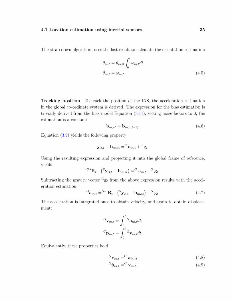
Tracking position To track the position of the INS, the acceleration estimation
in the global co-ordinate system is derived. The expression for the bias estimation is
trivially derived from the bias model Equation (3.11), setting noise factors to 0, the
estimation is a constant
bin,at = bin,a(t−1). (4.6)
Equation (3.9) yields the following property
yA,t − bin,at =S ain,t +S gt.
Using the resulting expression and projecting it into the global frame of reference,
yieldsGSRt ·
(SyA,t − bin,at
)=G ain,t +G gt.
Subtracting the gravity vector Ggt from the above expression results with the accel-
eration estimation.Gain,t =GS Rt ·
(SyA,t − bin,at
)−G gt. (4.7)
The acceleration is integrated once to obtain velocity, and again to obtain displace-
ment:
Gvin,t =
∫ t
0
Gain,tdt;
Gpin,t =
∫ t
0
Gvin,tdt.
Equivalently, these properties hold
Gvin,t =G ain,t; (4.8)Gpin,t =G vin,t. (4.9)

36 Location estimation
4.1.2 Domain-specific assumptions - the orientation kalman
filter
In some applications it is possible to make assumptions about the movement of the
body to which the IMU is attached [41]. Such assumptions can be used to minimize
drift. The kalman filter presented in this section uses assumptions of human body
motion to detect orientation drift errors. The filter is based on the work of Luinge
et al. [43] which presents an optimum filter for measuring human body segments
orientation using INS sensors. The filter overcomes gyroscope drift problems by
correcting the estimation using the acceleration data.
This section contains a detailed overview of the kalman filter. We present a
different derivation than specified in [43], the resulting matrices are much simpler
while preserving performance. The following is a concise description of the derivation,
please refer to the original paper for more details.
Sensor fusion using kalman filter
Orientation is estimated using a complementary kalman filter, using 3D accelerometer
and 3D gyroscope systems. The structure of the kalman filter is shown in Figure
4.3. Each of the sensor systems is used to derive an independent estimation of the
inclination, with different accuracy and error sources( Z−A for accelerometer and Z−Gfor gyroscope). The difference between the estimations ( Z−A − Z−G) is modeled as
a function of errors in the measurements, specifically gyroscope orientation error,
gyroscope bias error and measurements noise. This function is the error model which
,when converted to state space format, serves as the basis for the kalman filter.
Model of sensor signals
The sensor unit is attached to a human body, hence the model is based on character-
istics of human motion. The main assumption states that the acceleration of a body
segment in the global reference frame can be described as a low pass filtered white
noise. It relies on the fact that the body segment can’t be going in the same direction
for too long, it will hit a wall after some time.
The gyroscope signal and bias are modeled as described in Equation (3.4) and
Equation (3.6). The accelerometer signal is modeled as the sum of the acceleration
vector S~at,the gravity vector and white gaussian measurement noise vA,t. All vectors

4.1 Location estimation using inertial sensors 37
Figure 4.3: Structure of the kalman filter. Two estimations of the inclination areused, Z−G and Z−A. The difference between them is a function of the orientation and
bias errors (θε, bε) which the kalman filter estimates. The uncertainties of the mea-surements and model are expressed in terms of covariances, Qb for bias uncertainty,Qθ for orientation uncertainty and QZG ,QZA for inclination uncertainties
Figure 4.4: Sensor model diagram. The diagram details the components of eachsignal (yG and yA) and the relationships between them. Gyroscope signal is modeledas the angular velocity component ω, a white noise component vG and a slowlyvarying gyroscope bias wb. The orientation GSR is computed from the gyroscopesignal using the box ’strapdown integration’. Acceleration is modeled as a low passedfiltered white noise wa. The acceleration signal yA is composed of the accelerationand gravity vector relative to the sensor’s frame (Sa−S g) plus a white measurementnoise vb
are in the sensor’s reference frame.
yA,t =S at −S gt + vA,t.

38 Location estimation
The acceleration vector is modeled as a first order low-pass filtered white noise process.
The model is based on the assumption that during human motion, the acceleration
vector changes constantly and is much smaller than the gravity vector.
Gat = ca · Gat−1 + wa,t. (4.10)
Note this is a simplified model compared to Equation (3.9). Bias effects are neglected
and acceleration itself is modeled as a simple random process. Since this filter is only
aimed at improving orientation estimates, this simple model suffices.
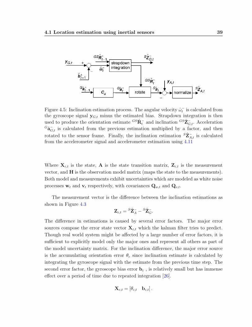
Inclination estimation
Based on the sensor model, the inclination estimation process for both the gyroscope
and accelerometer systems can be described. Figure 4.5 shows the estimation process,
based on the sensor model previously described. The acceleration Ga−t , gyroscope bias
b−t and angular velocity ω−t are calculated using equations 4.10, 3.6 and 3.4 respec-
tively while setting the noise factors to zero. The orientation estimation GSR−t is
calculated by strapdown integration of the previous orientation estimate GSR+t−1, to-
gether with the current angular velocity ω−t . Inclination estimation SZ−G,t can then be
extracted from the orientation matrix. For the accelerometer system, the acceleration
estimate is calculated in the sensor frame Sa−G,t and subtracted from the sensor signal
yA,t to receive the gravity vector (according to Equation (3.9)). The gravity vector
is then normalized and negated to produce the estimation of inclination SZ−A,t.
SZ−A,t =yA,t −S at|yA,t −S at|
. (4.11)
Error model
A complementary kalman filter uses a state space model representation to model
the relationship between the model state variables Xε,t (the error sources) and the
inclination error predicted by the model [69].
Xε,t = A · xε,t−1 + wt
Zε,t = H · xε,t + vt. (4.12)
4.1 Location estimation using inertial sensors 39
Figure 4.5: Inclination estimation process. The angular velocity ω−t is calculated fromthe gyroscope signal yG,t minus the estimated bias. Strapdown integration is then
used to produce the orientation estimate GSR−t and inclination GSZ−G,t. AccelerationGa−G,t is calculated from the previous estimation multiplied by a factor, and then
rotated to the sensor frame. Finally, the inclination estimation SZ−A,t is calculatedfrom the accelerometer signal and accelerometer estimation using 4.11
Where Xε,t is the state, A is the state transition matrix, Zε,t is the measurement
vector, and H is the observation model matrix (maps the state to the measurements).
Both model and measurements exhibit uncertainties which are modeled as white noise
processes wt and vt respectively, with covariances Qw,t and Qv,t.
The measurement vector is the difference between the inclination estimations as
shown in Figure 4.3
Zε,t = SZ−A −SZ−G.
The difference in estimations is caused by several error factors. The major error
sources compose the error state vector Xε,t which the kalman filter tries to predict.
Though real world system might be affected by a large number of error factors, it is
sufficient to explicitly model only the major ones and represent all others as part of
the model uncertainty matrix. For the inclination difference, the major error source
is the accumulating orientation error θε since inclination estimate is calculated by
integrating the gyroscope signal with the estimate from the previous time step. The
second error factor, the gyroscope bias error bε , is relatively small but has immense
effect over a period of time due to repeated integration [26].
Xε,t = [θε,t bε,t] .

40 Location estimation
Error propagation The bias prediction error can be found by using the bias model
3.6 and the bias prediction equations.
b−ε,t = b−t − bt
= b−t−1 − bt−1 −wb,t
= b−ε,t−1 −wb,t. (4.13)
The orientation error propagation is given by
θ−ε,t = θ−ε,t−1 −Tb−ε,t−1 + TvG,t. (4.14)
Using these results 4.13 and 4.14, the state transition equations can be written in
matrix form: (θε,tbε,t
)=
[1 −T0 1
]·
(θε,t−1
bε,t−1
)+
(TvG,t−wb,t
)
Xε,t =
[1 −T0 1
]·Xε,t−1 +
(TvG,t−wb,t
). (4.15)
Error covariance matrix Qw,t can be easily produced. The noise processes are inde-
pendent, so the covariance matrix becomes a simple diagonal matrix.
Qw,t =
[T 2QvG 0
0 Qbg
]. (4.16)
Where QvG is the gyroscope noise covariance matrix and Qbg is the very small co-
variance matrix of the bias noise.
Relationship between filter inputs and error states The error of the gyroscope
based inclination estimate can be obtained from the formula [60]
GSR = GSR · (I + [θε×] (4.17)

4.1 Location estimation using inertial sensors 41
Since the inclination SZ−G is simply one of the rows of the rotation matrix, the same
relationship holds (for small errors)
SZ−G = SZ−G · (I + [θε×]) (4.18)
The accelerometer-based inclination estimate SZ−A depends on the error in esti-
mated acceleration and the accelerometer sensor noise. Since the acceleromter is
expressed in the sensor co-ordinate system, orientation error is also a possible error
factor. The error in predicted acceleration in the global co-ordinate system can be
found by using Equation (4.10)
Ga−ε,t =G a−t −G at
= ca · Ga−t−1 − (ca · Gat−1 + wa,t)
= ca · Gaε,t−1 −wa,t. (4.19)
In order to calculate Sa−ε,t in the sensor frame, the Equation (4.17) is used to com-
pensate for orientation errors
Sa−ε,t = ca · Saε,t−1 − Swa,t +S a−t × θε,t. (4.20)
To obtain the accelerometer-based inclination estimate, Equation (3.9) is used to-
gether with Equation (4.20)
yA,t −S at =S at −S gt + vA,t −S at
=S aε,t −S gt + vA,t
= ca · Saε,t−1 − Swa,t +S a−t × θε,t −S gt + vA,t.
Putting it all together and using Equation (4.11) gives the following result
SZ−A,t = Zt +1
g
(ca · Saε,t−1 +S a−t × θε,t − Swa,t + vA,t
). (4.21)
Where the magnitude of acceleration is approximated by g the gravitational force.
The difference between inclination estimates can be expressed using the error state

42 Location estimation
variables using Equations 4.11 and 4.18.
SZε,t = SZ−A,t −SZ−G,t
=
(SZt −
Sa−tg
)× θε,t +
1
g
(ca · Saε,t−1 − Swa,t + vA,t
)=
[(SZt −S a−tg
)×] . . .
0
. . .
·(θε,t
bε,t
)+ vt.
Where the noise term vt is described by
vt =1
g
(ca · Saε,t−1 − Swa,t + vA,t
). (4.22)
The matrix H is a 3× 6 matrix
H =
[(SZt −S a−tg
)×] 0 0 0
0 0 0
0 0 0
. (4.23)
Finally, the covariance matrix of the measurement noise can be derived from
Equation (4.22)
Qv,t =1
g2
(c2a ·Q+
a,t−1 + Qwa + Qva
).
Where Q+a,t−1 is the aposteriori acceleration error covariance matrix. Qwa is the
covariance matrix of wa,t and Qva is the covariance matrix of vA,t.
4.2 Location estimation using RSSI
RSSI-based tracking systems use Received Signal Strength Indication (RSSI) to get an
estimate of the distance between transmitter and receiver (ranging) [49]. Estimations
rely on a network of static anchor nodes, which measure the RSSI from the moving
object. The main challenge is inferring the distance from the signal strength. It is
not easy to model the radio propagation in the indoor environment because of severe
multipath, low probability for availability of line-of-sight (LOS) path, and specific site
parameters such as floor layout, moving objects, and numerous reflecting surfaces [70].
Using distance estimations from 2 or more anchor nodes (for 2D), the location can be

4.2 Location estimation using RSSI 43
determined using triangulation or scene analysis. Triangulation (also known as range-
based RSSI) directly estimates the distance from the signal strength measurements
and combines them to compute the object location. This method is more straight
forward but is prone to large errors due to shadowing effects. On the other hand, scene
analysis refers to algorithms that first collect features (fingerprints) of a scene and
then estimate the location of an object by matching online measurements with the
closest a priori location fingerprints [48]. The fingerprinting algorithms have usually
two stages, an offline calibration stage and the online stage. During the offline stage,
a site survey is performed. The location coordinates and respective signal strengths
from the anchor nodes are collected. During the online stage, the currently observed
signal strengths are used to locate the object according to the previously recorded
map.
The RSSI-based algorithm used in this research is a described in detail in previ-
ous work by Blumrozen et al. [16]. The algorithm uses an innovative fingerprinting
method to tune the channel model parameters. During the offline stage, the opti-
mal transmission power is determined. Maximizing the dynamic range of the RSSI
measurements can lead to significant improvement in estimation accuracy [71]. Insuf-
ficient transmission power may lead to high packet loss while high transmission power
can lead to saturation of the RSSI measurements and distort the distance estimation.
The dynamic range is adaptively determined using a new method described in [16].
The second part of the offline stage is the calibration process which is based on log
fitting of the RSSI measurements and approximating the power offset and the channel
exponent.
During the online stage, RSSI measurements are collected and preprocessed. First,
measurements from the various nodes are synchronized. Second, the range is esti-
mated using the Equation (3.14)
Lrti = Lt+ A− q10 log10 dti + αt. (4.24)
Finally, the location is estimated using trilateration, based on a method described in
[72]. Each range estimation forms a circle around the anchor node, these circles have
two intersection points. Choosing the closest point to the object location satisfies the
Maximum A Posteriori criterion. This is illustrated in Figure 4.6.

44 Location estimation
Figure 4.6: Selecting the intersection point closest to the object location
4.3 Location estimation using sensor fusion
This section describes the design of an optimum filter for location estimation using
sensor data fusion as presented in Figure 4.7. The filter uses inertial sensors data and
estimates location using strap down integration as outlined in Section 4.1. RSSI data
is used as a second source of location information and an estimate is calculated as
detailed in Section 4.2. The process of optimally fusing the two location estimations
is performed using a kalman fitler.
A complementary kalman filter is designed to estimate positioning, velocity and
orientation errors. As illustrated in Figure 4.7 the filter uses two independent esti-
mations of location, each with different accuracies and error sources. The positioning
difference p−INS − p−RSSI is modeled as a function of errors in both measurement sys-
tems, particulary location,velocity and orientation errors in the gyroscope system.
The system uses a feedback design to constantly fix the inertial system estimations
according to the kalman filter corrections. Future work will also include feedback to
the RSSI system, enabling online-calibration.
Error model
As explained above in 4.1.2, a complementary kalman filter uses a state space model
representation to model the relationship between the model state variables Xε,t (the
error sources) and the error predicted by the model. The general state space model

4.3 Location estimation using sensor fusion 45
𝑄𝑣𝑅,𝑄𝑤𝑅
𝑄𝑣𝐴 ,𝑄𝑣𝐺,𝑄𝑤𝑎,𝑄𝑤𝐺 ,𝑄𝜃
𝑝 𝜀 ,𝑣 𝜀 ,𝜃 𝜀 ,𝑏 𝑎,𝜀,𝑏 𝑔,𝜀
accelerometer
s ignal
RSSI data 𝒑 𝑹𝑺𝑺𝑰−
𝒑 𝑰𝑵𝑺−
RSSI node
RSSI system
gyroscope
s ignal
Shimmer sensor
INS system
Kalman
fi lter
RSSI node
Figure 4.7: Top level design of the system. The system is composed of two indepen-dent sub systems that estimate the location, the kalman filter estimates the errorsand corrects them using a feedback loop. Two estimations of the location are used,p−INS and p−RSSI . The difference between them is a function of the location,velocity,
orientation and bias errors (pε, vε, θε, ba,ε, bg,ε) which the kalman filter estimates. Theuncertainties of the measurements and model are expressed in terms of covariances,Qwa and Qwg for bias uncertainties, QvA and QvG for sensor white noise ,QvR forRSSI estimation uncertainties and Qwr for RSSI shadowing uncertainties
representation was described in Equation (4.12).
The measurement vector is the difference between the location estimations as
depicted in Figure 4.7
Zε,t = p−in − p−rssi. (4.25)
The difference in location estimations is modeled as a function of several error sources.
These errors compose the error state vector Xε,t which the kalman filter tries to pre-
dict. For the location difference, the dominant error factors are the notorious inertial
navigation systems caveats - integration drift and sensor bias [26]. The inertial sys-
tem estimates location by integrating orientation, velocity and location, each integral
is a potential error source due to integration drift (θε, vε, pε respectively). The second
factor to consider is sensor bias error. Although the bias offset is very small, if not
mitigated it might cause large errors due to repeated integration of error each time
step [26]. ba,ε and bg,ε represent the accelerometer bias error and gyroscope bias

46 Location estimation
error, respectively.
Xε,t =[pε, vε, θε, ba,ε, bg,ε
]. (4.26)
The error state variables that compose Xε,t are defined as follows. pε is the difference
in location between the real location and estimated location by the inertial system
pε = pin,t − pt. (4.27)
Similarly, the variable vε is the difference between velocity estimations
vε = vin,t − vt. (4.28)
The orientation difference θε is defined to be the rotation vector between the
estimated rotation and the real rotation. Recall for small rotations, the relation
between orientations is given by Equation (3.3). Hence, the following formula can be
derived
RGSin,t = RGS
t
(I +
[θε×
]). (4.29)
Another form of this property can be written in terms of rotation vectors, where
θin,t,θt are the rotation vectors equivalent to RGSin,t, R
GSt respectively.
θε = θin,t − θt. (4.30)
Finally, the state variables corresponding to bias errors ba,ε, bg,ε are simply defined
as
ba,ε = ba,ins − ba
bg,ε = bg,ins − bg. (4.31)
Error propagation The error propagation equations are derived in continuous
time and are later transformed to discrete time. Using continuous time, the derivation
is simpler and more intuitive since human motion is a physical continuous process.
When using continuous terms, the error propagation equations express the derivative
of the variables.
First, the variable pε is examined. By definition, it is simply the difference between
the estimated and real location [see Equation (4.27)]. Calculating the derivative is
4.3 Location estimation using sensor fusion 47
trivial and gives the following result
pε = pin,t − pt= vin,t − vt
= vε. (4.32)
Where the last result was derived according to Equation (4.28). The derivation for
vε is similar
vε = vin,t − vt= ain,t − at
= aε. (4.33)
Where aε is defined to be the difference between acceleration estimations. This vari-
able is not a state variable, as it is expressed by θε as the following derivation shows.
Recall from Equation (4.7) that
Gain,t = GyA,t − GSRin,tSbin,at +G gin,t. (4.34)
Substituting SyA,t according to Equation (3.9) yields
GyA,t = RGSin,t ·
(Sat −S gt + ba,t + vA,t
).
Using Equation (4.29) for the variable RGSin,t
GyA,t = RGSt ·
(I +
[θε×
])·(Sat −S gt
)+RGS
in,t · ba,t +RGSin,t · vA,t
= RGSt · Sat −RGS
t · Sgt + θε × Sat − θε × Sgt +RGSin,t · ba,t +RGS
in,t · vA,t= Gat − Ggt + θε × Sat − θε × Sgt +RGS
in,t · ba,t +RGSin,t · vA,t. (4.35)
Returning to the Equation (4.33) and substituting Gain,t according to Equation (4.34)
yields
aε = GyA,t − GSRin,tSbin,at +G gin,t − at.

48 Location estimation
Using the result 4.35 from above , the following can be derived
aε = θε × Sat − θε × Sgt +RGSin,t ·
(ba,t − Sbin,at
)+RGS
in,t · vA,t= θε
([Sat×
]−[Sgt×
])−RGS
in,t · ba,ε +RGSin,t · vA,t. (4.36)
Where the last transition was according to the definition of ba,ε in Equation (4.31).
For the variable θε, using Equation (4.30) yields
θε = ˙θin,t − θt. (4.37)
Recall Equations 4.3 and 4.5 for ˙θin,t and θt
˙θin,t = yG,t − bin,gt
θt = ωt.
Substituting these properties to Equation (4.37) yields
θε = yG,t − bin,gt − ωt.
yG,t can be replaced according to Equation (3.4)
θε = ωt + bgt + vG,t − bins,gt − ωt= −bε + vG,t. (4.38)
Where the last result is derived using 4.31 Finally, for the bias error derivative, recall
Equations 3.13 and 3.8
ba,t = wba,t
bg,t = wbg,t. (4.39)
Using also Equations 4.1 and 4.6 we get
bin,at = 0
bin,gt = 0.
Where the derivative is zero since the estimation is a constant. Substituting these

4.3 Location estimation using sensor fusion 49
expressions in the bias error definition, yields -
ba,ε = ˙ba,ins − ba
= −wba,t
bg,ε = ˙bg,ins − bg
= −wbg,t.
Let us summarize the linear differential equations obtained so far,
pε = vε
vε = θε([Sat×
]−[Sgt×
])−RGS
in,t · ba,ε +RGSin,t · vA,t
θε = −bε + vG,t
ba,t = −wba,t
bg,t = −wbg,t.
According to Equations 4.32,4.36, 4.39,4.38 for location,velocity,bias and orientation
errors respectively. Writing these equations in matrix representation, yieldspεvεθε
bg,tba,t
= Acont
pεvεθε
bg,tba,t
+
0
vA,tvG,t−wbg,t
−wba,t
. (4.40)
Where all variables are three dimensional vectors and Acont is a 15× 15 matrix.
Acont =
0 I 0 0 0
0 0([Sat×
]−[Sgt×
])0 −RGS
in,t
0 0 0 −I 0
0 0 0 0 0
0 0 0 0 0
. (4.41)
Where 0 denotes a 3× 3 zero matrix and I is a 3× 3 unity matrix.
Since the sensors sample the process in discrete times, we shall transform the

50 Location estimation
equations to discrete-time dynamics. Recall that [66] for a continuous time linear
system given by the dynamics
x = Bx
y = Cx.
The transformation to discrete time dynamics is given by
xt = eB∆txt−1
yt = Cxt. (4.42)
Where eAcont∆t can be calculated using the formula [73]
eBt =∞∑j=0
(Bt)j
j!.
For the state transition matrix Acont described in 4.41, the summation terms Aicont
can be easily computed as follows
A0cont = I
A2cont =
03 0
([Sat×
]−[Sgt×
])0 −RGS
in,t
0 0 0 −([Sat×
]−[Sgt×
])0
0 0 0 0 0
0 0 0 0 0
0 0 0 0 0
A3cont =
0 0 0 −
([Sat×
]−[Sgt×
])0
0 0 0 0 0
0 0 0 0 0
0 0 0 0 0
0 0 0 0 0
A4cont = 0.

4.3 Location estimation using sensor fusion 51
Thus, the formula for eAcont∆t is given by
eAcont∆t = A0cont + A1
cont∆t+ A2cont
∆t2
2+ A3
cont
∆t3
6I ∆t · I ∆t2
2
([Sat×
]−[Sgt×
])−∆t3
6
([Sat×
]−[Sgt×
])−∆t2
2RGSin,t
0 I ∆t([Sat×
]−[Sgt×
])−∆t2
2
([Sat×
]−[Sgt×
])−∆tRGS
in,t
0 0 I ∆t3 0
0 0 0 I 0
0 0 0 0 I
.(4.43)
Using the discrete time transformation Eq.4.42 with the continuous time dynamics
system Eq.4.40 gives us the following discrete time dynamics system for error propa-
gation - pε,tvε,tθε,tbg,tba,t
= A
pε,t−1
vε,t−1
θε,t−1
bg,t−1
ba,t−1
+
0
vA,tvG,t−wbg,t
−wba,t
∆t. (4.44)
Where A is an 15× 15 matrix as described in Equation (4.43). Note that the matrix
A depends on current acceleration and orientation of the object, thus it is recomputed
each cycle of the filter.
The model noise covariance matrix can be easily computed, since it is composed
of independent white noise processes.
Qw,t =
0 0 0 0 0
0 ∆t2QvA 0 0 0
0 0 ∆t2QvG 0 0
0 0 0 ∆t2Qwg 0
0 0 0 0 ∆t2Qwa
(4.45)
where QvG,QvA, Qwg,Qwa are white noise process covariance matrices as defined in
Eq. (3.5),Eq.3.10,Eq.3.7,Eq.3.12 respectively.

52 Location estimation
Relationship between filter input and error states The error of the RSSI
based location estimate is given by Equation (3.15)
prssi,t = pt + br,t + vR,t. (4.46)
Where pt is the real location, br,t is a correlated noise process and vR,t a white noise
gaussian process. The expression for the location estimation difference was found by
substituting Eq.4.46 and Eq.4.27 into Eq.4.25
Zε,t = p−in − p−rssi
=(p−in − pt
)−(p−rssi − pt
)= pε − (br,t + vR,t) .
Rewriting the last equation according to the kalman filter formulation, yields
Zε,t =[I 0 0 0 0
]Xε,t − (br,t + vR,t) . (4.47)
Where I is a 3× 3 identity matrix, 0 is a 3× 3 zeros matrix and Xε,t is the error state
vector defined in Equation (4.26).
Kalman filter can be derived to work with colored measurement noise process by
augmenting the state vector with the noise process [67]. This derivation is needed
since the measurement noise expression (br,t + vR,t) in Equation (4.47) contains corre-
lated components and thus does not comply with the basic kalman filter assumptions
of white noise processes only. Recall from Equation (3.17) that the correlated noise
process model is
br,t = e−|∆t|τ br,t−1 + wr,t. (4.48)
Augmenting the state vector from Eq. (4.44) with the noise process given in Eq.
(4.48) yields the state space representation of the kalman filter
X′ε,t = A′X′ε,t−1 +
0
vA,tvG,t−wbg,t
−wba,t
wbr,t
∆t.

4.3 Location estimation using sensor fusion 53
Where X′ε,t is the augmented state vector
X′ε,t =
pε,tvε,tθε,tbg,tba,tbr,t
.
A′ is the augmented state transition matrix of size 18× 18 given by
A′ =
I ∆t · I ∆t2
2
([Sat×
]−[Sgt×
])−∆t3
6
([Sat×
]−[Sgt×
])−∆t2
2RGSin,t 0
0 I ∆t([Sat×
]−[Sgt×
])−∆t2
2
([Sat×
]−[Sgt×
])−∆tRGS
in,t 0
0 0 I ∆t3 0 0
0 0 0 I 0 0
0 0 0 0 I 0
0 0 0 0 0 e−|∆t|τ I
.
The relationship between filter inputs and error states was found be rewriting
Eq.4.47 with the augmented state vector
Zε,t =[I 0 0 0 0 −I
]X′ε,t − vR,t.
The model noise covariance matrix was found by augmenting the covariance matrix
4.45 with the wbr,t noise process which is independent of the other noise processes,
yielding
Qw,t =
0 0 0 0 0 0
0 ∆t2QvA 0 0 0 0
0 0 ∆t2QvG 0 0 0
0 0 0 ∆t2Qwg 0 0
0 0 0 0 ∆t2Qwa 0
0 0 0 0 0 ∆t2Qwr
.

54 Location estimation
Where Qwr is the covariance matrix of wbr,t as defined in Eq. (3.18). The measure-
ment noise covariance matrix is simply given by
Qv,t =[QvR
].
Where QvR is the covariance matrix of vR,t as defined in Eq. (3.16).

Chapter 5
Experimental methods
Experiments were conducted to verify the effectiveness and robustness of the track-
ing filter. The experiments were carried out on a 50 × 50 cm surface in an indoor
environment. The experiments aim was to track the position of a moving hand, along
the surface of the table, as depicted in Figure 5.1.Data was collected in real-time and
post-processed using a program written in Matlab. Sampling rate was approximately
50 Hz. The tracking results were tested by comparison of the location estimation to
the location information that was obtained by a laboratory-bound 3D optical tracking
system Polaris [74].
The experiment design is presented in Figure 5.2. The sensors data is acquired and
calibrated as explained in Section 5.4. The data is then synchronized and interpolated
to create a uniform time stamp and sampling rate, see Section 5.5 for more details.
Finally, location is estimated as explained in 4. The results are compared to the
reference tracking data provided by the polaris system.
5.1 Experiment setup
The experiment setup is depicted in Fig. 5.1. Inertial movement information was
acquired using a SHIMMER sensor attached to the moving hand [75]. For RSSI
measurements, two BSN sensor nodes [76] were used as anchor nodes, and the third
was used as a mobile node. Location estimation was accomplished by fusion of both
sensor systems.
The current implementation of the RSSI tracking system consists of only 2 anchor
nodes, thus providing only 2D tracking capability. Hence, the experiments were
limited to 2D movement across the experiment area. Intensive simulation testing was
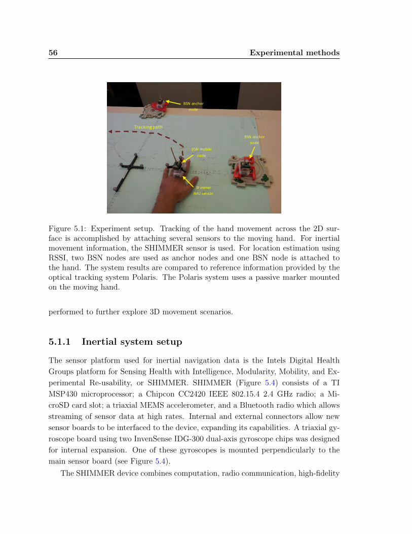
56 Experimental methods
BSN anchor
node
BSN anchor
node
Tracking path
BSN mobile
node
Shimmer
IMU sensor
Figure 5.1: Experiment setup. Tracking of the hand movement across the 2D sur-face is accomplished by attaching several sensors to the moving hand. For inertialmovement information, the SHIMMER sensor is used. For location estimation usingRSSI, two BSN nodes are used as anchor nodes and one BSN node is attached tothe hand. The system results are compared to reference information provided by theoptical tracking system Polaris. The Polaris system uses a passive marker mountedon the moving hand.
performed to further explore 3D movement scenarios.
5.1.1 Inertial system setup
The sensor platform used for inertial navigation data is the Intels Digital Health
Groups platform for Sensing Health with Intelligence, Modularity, Mobility, and Ex-
perimental Re-usability, or SHIMMER. SHIMMER (Figure 5.4) consists of a TI
MSP430 microprocessor; a Chipcon CC2420 IEEE 802.15.4 2.4 GHz radio; a Mi-
croSD card slot; a triaxial MEMS accelerometer, and a Bluetooth radio which allows
streaming of sensor data at high rates. Internal and external connectors allow new
sensor boards to be interfaced to the device, expanding its capabilities. A triaxial gy-
roscope board using two InvenSense IDG-300 dual-axis gyroscope chips was designed
for internal expansion. One of these gyroscopes is mounted perpendicularly to the
main sensor board (see Figure 5.4).
The SHIMMER device combines computation, radio communication, high-fidelity

5.1 Experiment setup 57
𝒑 𝒑𝒐𝒍𝒂𝒓𝒊𝒔
Compare
Polaris Sensor input
sync
data
𝒑 𝜺
Location Estimation
𝒑 𝑰𝑵𝑺+
𝒑 𝑰𝑵𝑺−
Data Processing
BSN nodes
input
Shimmer
input
sync
data 𝒑 𝑹𝑺𝑺𝑰
−
Estimation by INS
Pre-process
Kalman
fi l ter
calibrate
Pre-
process
calibrate
Estimation by RSSI
Figure 5.2: Block diagram of the experiment data flow. Sensor data from the SHIM-MER and BSN node is calibrated and pre-processed. All data sources are synchro-nized, and a uniform time stamp is determined. The location estimation process iscomposed of the INS and RSSI location estimations (p−INS and p−RSSI respectively).The kalman filter uses both estimations to predict the errors pε. The INS errors arecorrected in a feedback loop and the location estimation is computed p+
INS. Polarislocation estimation ppolaris is then compared to results and the Mean Squared Erroris calculated.
triaxial sensors, and a large flash memory into a tiny, wearable rugged plastic enclo-
sure. It measures 1.75 x 0.8 x 0.5 and weighs just 10 g.
5.1.2 RSSI system setup
The RSSI tracking was performed by two anchor nodes placed at x and y axes and a
third node attached to the moving hand. The mobile node transmitted data packets.
The anchor nodes received the packets and calculated the RSSI measurements.
The wireless nodes are composed of a BSN node [76] and a dipole antenna. A BSN
node includes a processing unit (TI MSP430) and a wireless chip (Chipcon CC2420)
[77]. The wireless transceiver has a built-in RSSI that provides a digital value in the
range of −127 to 128 dBm. An omnidirectional antenna was added to each node
to increase the transmission range. The antenna was made by bending and winding
together a 10 cm wire and forming a dipole antenna of 5 cm, which is equivalent to
half the length of the 802.15.4a wave length.

58 Experimental methods
BSN anchor
node
Dipole
antenna
BSN node
Shimmer
IMU sensor
Polaris
marker
Figure 5.3: The mobile node attached to the hand. A SHIMMER sensor is used forcapturing INS information, a BSN node transmits data packets for RSSI measure-ments and a Polaris passive marker is used by the Polaris system to track the movinghand
Antenna
3 axis
Gyroscope
3-axis
Accelerometer
Li-ion battery
Wireless
transceiver
Figure 5.4: The SHIMMER wearable sensor platform. SHIMMER incorporates a TIMSP430 processor, a CC2420 IEEE 802.15.4 radio, a triaxial accelerometer, and arechargeable Li-polymer battery. A triaxial gyroscope board is added as an internalexpansion with two dual-axis gyroscope chips. The platform also includes a MicroSDslot supporting up to 2 GB of Flash memory

5.2 Comparison with optical tracking system 59
5.2 Comparison with optical tracking system
The polaris system is an optical measurement system that measures the 3D position
and orientation of either passive or active markers [74]. The system is highly accurate,
providing sub-millimeter accuracy for a limited range of operation. It is manufactured
by Northern Digital Inc. (NDI) of Waterloo, Ontario, Canada and is the leading
system used for Image Guided Surgery (IGS). The programming interface for the
polaris system is provided by the IGSTK, a software toolkit for image-guided surgery
applications [78].
The polaris system can instantaneously track up to 15 markers. The experiment
setup uses two passive markers, as depicted in Figure 5.2. A static marker is placed
in the origin of axis, position and orientation conforming with the co-ordinate system
defined by the RSSI tracking system. The second marker is attached to the moving
hand, tracking its position and orientation. The polaris system outputs the relative
movement of the mobile marker in the co-ordinate system defined by the static marker.
Polaris mobi le
marker
X Y
X
Y Polaris reference
marker
Z
Z
Figure 5.5: The polaris tracking setup. Two passive markers are used. The first is astatic marker, placed in the origin of axis defined by the RSSI tracking system. Thesecond is a mobile marker attached to the moving hand.
5.3 Model parameters estimation
Before the Kalman filter was used, the model parameters were determined. The sensor
noise variances QvA and QvG were found by taking the variance of the sensor signal

60 Experimental methods
while the sensor was lying still on the laboratory floor. The bias instability parame-
ters Qwa and Qwg were found using a technique known as Allan Variance [79].Allan
Variance is a time domain analysis technique originally designed for characterizing
noise and stability in clock systems. The technique can be applied to any signal to
determine the character of the underlying noise processes.More specifically, the bias
instability is the minimum value of the Allan deviation curve. For a full description of
the Allan Variance technique see [80]. The noise parameter of the RSSI error model
Qwr was chosen to give reasonable results while the filter was tested
5.4 Sensor calibration
SHIMMER device calibration Shimmer devices use MEMs transducers for kine-
matic sensing. The current generation has a lower price point than previous genera-
tions but suffers from errors that may be insufficient for many applications [3]. Most
prominent errors are offset errors that are be caused by offset variations from trim
errors, mechanical stresses from the package and mounting, shifts due to temperature
and due to aging. These variables can all change the offset. The other source of
errors is scaling errors which affect the slope of the transfer function. The aim of the
calibration process is to eliminate these errors.
Figure 5.6: Transfer function of the accelerometer sensor. S is the slope of the transferfunction.VOFF is the offset error.
The calibration process is performed for both accelerometers and gyroscopes at
the beginning of each experiment session. Hence, it is required to be quick and

5.4 Sensor calibration 61
simple. The calibration scheme presented in this research is composed of one combined
calibration sequence for calibrating all sensors (3 axis accelerometer, 3 axis gyroscope).
The sequence is composed of steps, during each step the sensor is layed on one of its
faces, every step is at least 2 seconds long. Changing from one position to the other,
should be done by turning the sensor along one of its gyroscope axis. The calibration
code automatically computes the steps and turns, so all that is required from the user
is to traverse between all different faces and turns at least once, order doesn’t matter.
Accelerometer calibration is simple, given two points on the transfer function
(approximated as linear function), the slope and offset can be computed. As shown
in Figure 5.7 the calibration code locates the steps and finds for each step the earth-
facing sensor (only one axis measures g or −g at each time step). To reach an
approximation for −g all measurements from relevant steps are averaged (xaccmin) .
The same process repeats for +g (xaccmax ) for each axis. The two points on the slope
are (−g, xaccmin) and (+g, xaccmax) where g is the gravity force. The previously described
process is not accurate since the measured surface is never exactly aligned to the
ground, hence the measured force is not g , it is
gsurface = g cos (α) . (5.1)
Where α is the surface incline angle. The calibration process estimates the slope
incline (α) by calculating the acceleration measured by the two other sensors. The
following property holds (assuming z is earth facing)√a2x + a2
y = g sin (α) . (5.2)
Where ax and ay are the average values of the x and y sensors during one step. Solving
for α yields
α = arcsin
(√a2x + a2
y
g
). (5.3)
Substituting α in Equation (5.1) using 5.3 yields an estimation for gsurface which is
then used to run the calibration process again with the modified value.
The calibration results are validated using a validation sequence. The test se-
quence is composed of steps, on each step the sensor is placed in a static random
orientation in space. If the calibration is accurate, the total measured acceleration on
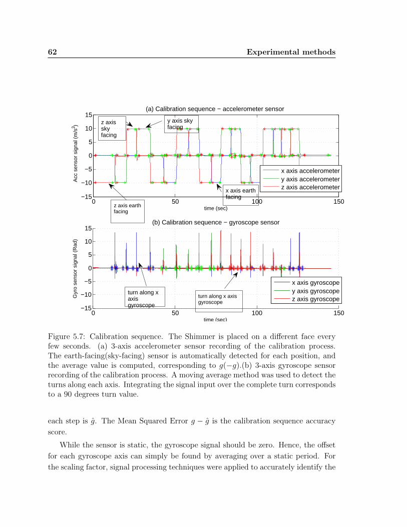
62 Experimental methods
0 50 100 150−15
−10
−5
0
5
10
15(a) Calibration sequence − accelerometer sensor
time (sec)
Acc
sen
sor
sign
al (
m/s
2 )
x axis accelerometery axis accelerometerz axis accelerometer
0 50 100 150−15
−10
−5
0
5
10
15(b) Calibration sequence − gyroscope sensor
time (sec)
Gyr
o se
nsor
sig
nal (
Rad
)
x axis gyroscopey axis gyroscopez axis gyroscope
z axisskyfacing
turn along xaxisgyroscope
z axis earthfacing
y axis skyfacing
x axis earthfacing
turn along x axisgyroscope
Figure 5.7: Calibration sequence. The Shimmer is placed on a different face everyfew seconds. (a) 3-axis accelerometer sensor recording of the calibration process.The earth-facing(sky-facing) sensor is automatically detected for each position, andthe average value is computed, corresponding to g(−g).(b) 3-axis gyroscope sensorrecording of the calibration process. A moving average method was used to detect theturns along each axis. Integrating the signal input over the complete turn correspondsto a 90 degrees turn value.
each step is g. The Mean Squared Error g − g is the calibration sequence accuracy
score.
While the sensor is static, the gyroscope signal should be zero. Hence, the offset
for each gyroscope axis can simply be found by averaging over a static period. For
the scaling factor, signal processing techniques were applied to accurately identify the

5.4 Sensor calibration 63
0 5 10 15 20 25 30 35 40 45 50
−10
−5
0
5
10
(a) Verification sequence − accelerometer sensor
time (sec)
Acc
sen
sor
sign
al (
m/s
2 )
x axisy axisz axisacc magnitude
0 5 10 15 20 25 30 35 40 45 509
9.5
10
10.5
11(b) Accelerometer magnitude compared with g
time (sec)
Acc
nor
m (
m/s
2 )
Acc magnitudeGravity force
Figure 5.8: Validation sequence. The sensor placed in a different static 3-D positionevery few seconds. The magnitude of the acceleration vector is expected to be thegravity force g. (a) The 3-axis accelerometer output and the calculated norm. (b)Comparison of the magnitude to the expected gravity. In the example there arefluctuations of 0.5m/s2 which might cause considerable errors.
time periods where the change in position took place. Each position change is a 90
degrees turn for one of the gyroscope sensors. Using Equation (4.4), the following
64 Experimental methods
can be derived ∫ t
0
yg,tdt =
∫ t
0
aωtdt = a
∫ t
0
ωtdt = aθπ2. (5.4)
Where yg,t is the gyroscope signal,a is the scaling factor, ωt is the angular velocity
and θπ2
represents a 90 degrees turn. Finally, the scaling factor a can be estimated by
integrating the gyroscope signal∫ t
0yg,tdt and extracting a from the previous formula.
RSSI calibration RSSI calibration process estimates the system parameters for
translating the power levels’ measurements between each pair of sensor nodes to
corresponding distance. RSSI measurements data is manually collected from a pre
determined set of points with known distances. The calibration scheme is based on log
fitting of the RSSI measurements and approximating the power offset and the channel
exponent using the a-priori knowledge of the environment physical dimensions and
the range of the channel exponent values. The calibration process is described in
detail in [16].
5.5 Data Synchronization
The measurements acquired from different sensor systems cannot be used together
without proper interpolation and synchronization.First, each data source has a dif-
ferent sampling frequency - the SHIMMER sensor operates in 208.4 Hrz, the mobile
BSN node transmits data packets in 52.1 Hrz and the polaris measurements are sam-
pled in 100 Hrz. Second, each data stream has a different time stamp, mandating the
use of an accurate synchronization algorithm to create a uniform time stamp.
The synchronization between the SHIMMER mote and the mobile BSN node was
accomplished by using the BSN’s on-board accelerometer sensor and comparing the
signal to the SHIMMER accelerometer sensor. The time delay estimation was found
by calculating the cross correlation function between the signals with varying offset
of one of them
c(k) = corr (absn (t) , ashimmer (t+ k)) . (5.5)
Where corr(a, b) is the cross correlation between a and b, absn (t) is the BSN ac-
celerometer signal and ashimmer (t+ k) is the SHIMMER accelerometer signal with a
k offset. The peak of the cross-correlation function is the time offset estimation.

5.5 Data Synchronization 65
0 5 10 15 20 25 30 35 40 45 50−20
−15
−10
−5
0
5
10
15
20
25Synchronization of Shimmer acceleromter with BSN accelerometer
time (sec)
Acc
sig
nal (
m/s
2 )
BSN accShimmer acc
Figure 5.9: Shimmer and BSN mobile node synchronization. Shimmer accelerometerand BSN accelerometer signals are shown after synchronization. Even though theBSN signal is not properly calibrated, the sync operation performs well.
The polaris system measurements were synchronized with the SHIMMER gyro-
scope measurements. The polaris system tracks both location and orientation of the
moving body. Recall Equation (4.5)
θin,t = ωin,t. (5.6)
The angular velocity is calculated from the orientation measurements by taking the
first derivative. Using the polaris estimation for angular velocity and the gyroscope
measurements by the SHIMMER the time offset can be found using the cross corre-
lation function as described in Equation (5.5).
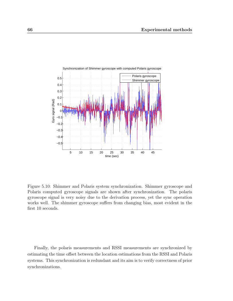
66 Experimental methods
5 10 15 20 25 30 35 40 45
−0.5
−0.4
−0.3
−0.2
−0.1
0
0.1
0.2
0.3
0.4
0.5
Synchronization of Shimmer gyroscope with computed Polaris gyroscope
time (sec)
Gyr
o si
gnal
(R
ad)
Polaris gyroscopeShimmer gyroscope
Figure 5.10: Shimmer and Polaris system synchronization. Shimmer gyroscope andPolaris computed gyroscope signals are shown after synchronization. The polarisgyroscope signal is very noisy due to the derivation process, yet the sync operationworks well. The shimmer gyroscope suffers from changing bias, most evident in thefirst 10 seconds.
Finally, the polaris measurements and RSSI measurements are synchronized by
estimating the time offset between the location estimations from the RSSI and Polaris
systems. This synchronization is redundant and its aim is to verify correctness of prior
synchronizations.

5.6 Analysis 67
5.6 Analysis
The filter performance analysis was split into several parts. First, Section 6.2 deals
with the main goal of the filter, location estimation. A number of real-world exper-
iments were conducted and trajectory estimations of the proposed filter were found.
Comparing the results to the RSSI-based system estimations, reveals great improve-
ment in discovering movement pattern but only slight improvement in the RMS sense
(see Fig. 6.3). Second, Sections 6.3 and 6.4 analyze the filter’s ability to track addi-
tional quantities such as Gyroscope and Accelerometer bias which are included in the
kalman state vector. These values are not the filter’s primary goal, but are interesting
and valuable by themselves. Gyroscope and Accelerometer bias are artificially added
to the experimental data, and the filter successfully tracks their value and detects dy-
namic changes. Section 6.3 further investigates the relationship between the kalman
parameters, dynamic response to changes and overall filter performance. The results
affirm the fact that filter parameters must be carefully set, since setting a value too
low causes slow dynamic response to change, and setting a value too high degrades
filter performance.
Finally, the third part (Section 6.5) validates the filter robustness to initial pa-
rameters errors. This is a critical parameter for assessing the quality of a filter,
since initial errors are common in real-world scenarios. Both location,velocity and
orientation errors are tested and successfully corrected.

Chapter 6
Results
The following sub-sections describe preliminary experimental results demonstrating
the accuracy of position estimation using the inertial/RSSI tracking system.
6.1 Parameter identification
An example of a gyroscope and accelerometer recording is given in Figure 6.1. It
shows the output signal of the shimmer sensor attached to a hand while moving on a
surface. It can be seen that the gyroscope signal suffers greatly from changing bias,
notice the decreasing signal magnitude in the first 5 seconds before the hand starts
moving. Static measurements with the sensors laying still on the laboratory table,
to obtain gyroscope and accelerometer noise, resulted in an RMS of 0.005 rads
and
0.05ms2
respectively. The time constant δt for the RSSI model as defined in Eq. (3.17)
was set to 5 s . It was determined by inspecting the change in RSSI bias during an
experiment as shown in Figure 6.2.
The filter initialization parameters are reported in Table 6.1. The values were
determined as explained above and extensively tested in simulation and experiments.
6.2 Typical results
Figure 6.3 shows results typical of the hand movement experiments for the kalman-
based filter and the RSSI-only system. The experiments varied in speed, length and
trajectory shape as can be seen. In each plot, both estimations are compared, with
the polaris output used as reference. The inertial system estimation is not shown

6.2 Typical results 69
5 10 15 20 25 30 35 40 45
−0.4
−0.2
0
0.2
0.4
0.6(a) Hand movement − accelerometer sensor
time (sec)
Acc
sen
sor
sign
al (
m/s
2 )
x axis accelerometery axis accelerometer
5 10 15 20 25 30 35 40 45
−0.4
−0.2
0
0.2
0.4
0.6(b) Hand movement− gyroscope sensor
time (sec)
Gyr
o se
nsor
sig
nal (
Rad
)
z axis gyroscope
Gyroscope bias
Figure 6.1: Measured sensor signals during one hand movement experiment (2D move-ment). (a) Accelerometer output vector, only x,y axis are shown since movement is2D. (b) Gyroscope output vector. The gyroscope changing bias can be seen in thefirst 10 seconds before the hand starts moving.
as it significantly diverges after just a few seconds. Figure 6.4 presents the filter
performance in a separate view for the x and y axis respectively. The three traces
in the upper plot represent the different estimations and the traces in the lower plot
represent the calculated error for each system. These plots reveal that, although both
systems are similar in MMSE sense, the proposed filter achieves far great accuracy in
estimating shape and pattern.
We use root mean squared error (RMSE) to compare a given trajectory {xn, yn, zn}and it’s estimated trajectory {xn, yn, zn}
RMSE =
√1
NΣNn=1
[(xn − xn)2 + (yn − yn)2 + (zn − zn)2] (6.1)

70 Results
5 10 15 20 25 30 35 40 45−0.2
−0.1
0
0.1
0.2
0.3
0.4RSSI location estimation error for x axis
time (sec)
Loca
tion
erro
r (m
)
RSSI location error − x axis
Figure 6.2: RSSI location error. The graph shows a changing bias with time constantof about 5 seconds. This constant is used to model the RSSI error.
Paramter value
QvG - Gyroscope sensor noise [defined in 3.5] 0.005 Radsec
Qwg - Gyroscope bias noise [defined in 3.7] 0.05 Rad/sec
QvA - Accelerometer sensor noise [defined in 3.10] 0.05 Msec2
Qwa - Accelerometer bias noise [defined in 3.12] 0.05 Msec2
Qwr - RSSI white noise [defined in 3.18] 0.1 Msec
δt - RSSI Time Constant [defined in 3.17] 5 sec
Table 6.1: Kalman filter initialization parameters.
Each RMS value was calculated for the whole duration of the experiment, neglect-
ing the first few seconds. This was to prevent errors due to initial convergence of the
filter. One way to measure the convergence of the Kalman filter is through examina-
tion of the trace of the error covariance matrix. Fig 6.5 shows the trace for one of
the experiments. It is noted that the sum of squared errors reaches a steady state
after approximately 10 s. The table 6.2 summarizes the RMS values of the location
estimation error for the INS, RSSI and the kalman filter. Each value, represents the
mean of all experiments. As the table shows, the kalman filter outperforms the other
system estimations. As expected, the inertial system suffers severely from drift and
its location error grows indefinitely. On the other hand, the kalman filter improves
the RSSI estimation only by a factor of 10-20 percent, this is due to the inaccuracy
of the inertial sensors output.

6.3 Gyroscope bias estimation 71
−0.4 −0.2 0 0.2 0.4−0.4
−0.2
0
0.2
0.4
x(M)
y(M
)
−0.3 −0.2 −0.1 0 0.1 0.2−0.4
−0.2
0
0.2
0.4
x(M)
y(M
)
Kalman−basedReal locationRSSI−only
−0.4 −0.2 0 0.2 0.4−0.4
−0.2
0
0.2
0.4
x(M)
y(M
)
−0.4 −0.2 0 0.2 0.4−0.4
−0.2
0
0.2
0.4
x(M)
y(M
)
Figure 6.3: Typical results for location estimations. Each plot shows the kalman-based,RSSI-based and reference estimations. Inertial-based estimation divergesquickly and is not presented.
6.3 Gyroscope bias estimation
The time required for the filter to estimate the offset was tested by off-line processing
of the sensor signals using an initial offset error, artificially added to the gyroscope
signals prior to application of the Kalman filter. The offset error at the end of the
measurement was then used as a measure for the ability of the filter to estimate the
offset.
An example of gyroscope bias estimation during an experiment is given in Fig.
6.6 The system successfully estimates the bias error and handles changes in bias
effectively. Fig 6.7 shows the performance of the kalman filter with a simpler model
for the gyroscope, without the bias. It is clearly shown that the full kalman filter
significantly outperforms the simple model. For the simple model, since the Gyroscope
bias is not compensated, the orientation error grows constantly, severely degrading
the filter performance.
The gyroscope bias instability value Qwg [defined in 3.7] has critical importance

72 Results
Estimation method Location error RMS (M)
Pure inertial system 34.8 [for 50 seconds experiment]. Unbounded.Pure RSSI-based system 0.0927Proposed filter (inertial and RSSI) 0.0808
Table 6.2: RMSE values for each estimation method. The kalman filter achievesgreater accuracy, improving the RSSI estimates by 10-20%
5 10 15 20 25
−0.2
−0.1
0
0.1
0.2
0.3
Time(sec)
X (
M)
(a) Location estimation of X axis
Kalman−basedReal locationRSSI−only
10 15 20 25 30
−0.05
0
0.05
0.1
0.15
Time(sec)
LEE
X (
M)
(b) Location error estimation of X axis
Kalman−basedRSSI−only
Figure 6.4: Typical results for location and location estimation error (LEE) decom-posed for X and Y axis. Plot (a) compares the location estimation of the proposedfilter with the RSSI-based estimation. The kalman filter tracks the movement andshape much better but overall RMS sense is quite similar as shown in plot (b).
for successfully handling changing bias values. Fig 6.9 shows filter behavior with
several different Qwg values. The value determines how quickly the filter can adapt
to changes in the bias, setting the value too low causes poor performance during a
rapid change. Unfortunately, setting the value too high comes with a price too, table
6.3 shows the RMS values for filter with different bias values. High bias value degrades
overall filter performance, even if no bias is present. Hence, for optimal performance
the Qwg value must be carefully set. Similar treatment to the other parameters of
the filter can be done but is not presented here due to shortage of space. In general,
for optimal filter performance, intricate tuning is needed.
The gyroscope bias estimation is limited. During static periods, the bias cannot
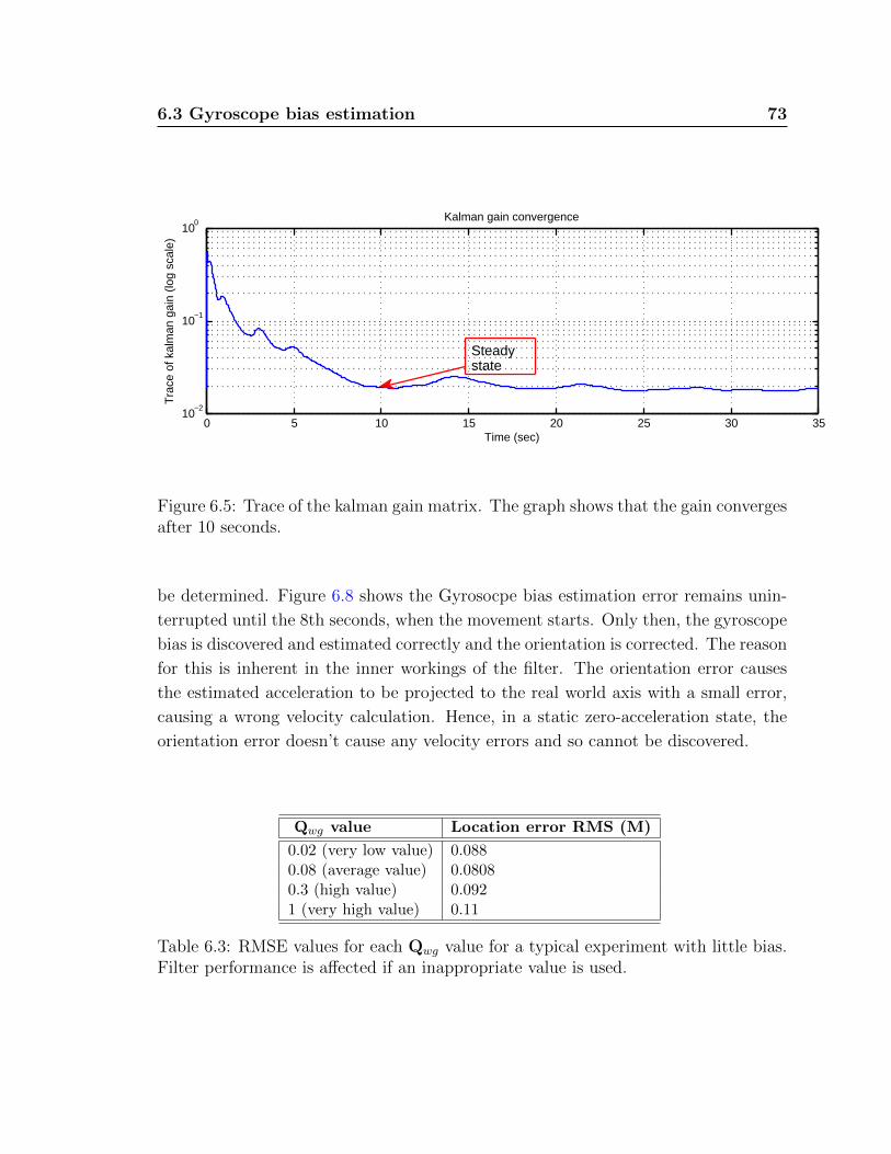
6.3 Gyroscope bias estimation 73
0 5 10 15 20 25 30 3510
−2
10−1
100
Time (sec)
Tra
ce o
f kal
man
gai
n (lo
g sc
ale)
Kalman gain convergence
Steadystate
Figure 6.5: Trace of the kalman gain matrix. The graph shows that the gain convergesafter 10 seconds.
be determined. Figure 6.8 shows the Gyrosocpe bias estimation error remains unin-
terrupted until the 8th seconds, when the movement starts. Only then, the gyroscope
bias is discovered and estimated correctly and the orientation is corrected. The reason
for this is inherent in the inner workings of the filter. The orientation error causes
the estimated acceleration to be projected to the real world axis with a small error,
causing a wrong velocity calculation. Hence, in a static zero-acceleration state, the
orientation error doesn’t cause any velocity errors and so cannot be discovered.
Qwg value Location error RMS (M)
0.02 (very low value) 0.0880.08 (average value) 0.08080.3 (high value) 0.0921 (very high value) 0.11
Table 6.3: RMSE values for each Qwg value for a typical experiment with little bias.Filter performance is affected if an inappropriate value is used.

74 Results
0 5 10 15 20 25 30 35
−0.05
0
0.05
0.1
0.15
Time(sec)
Rad
Gyroscope bias drift compensation
Estimated biasReal bias
0 5 10 15 20 25 30 35
−0.1
−0.05
0
0.05
Time(sec)
Rad
Gyroscope bias estimation error
Estimated bias error
Figure 6.6: Filter tracking of gyroscope bias drift. Plot (a) compares the estimatedGyroscope bias with the actual changing bias. Plot (b) shows the Bias EstimationError as a function of time.
6.4 Accelerometer bias estimation
The kalman filter models and successfully tracks the accelerometer bias. An example
for accelerometer bias estimation is found in Fig. 6.10. The figure clearly shows the
filter ability to track the changing accelerometer bias for both X and Y axis.
6.5 Sensitivity to initial condition errors
The system handles well initial errors for the location, velocity and orientation as
seen in Figures 6.11,6.12 and 6.13 respectively. For each plot, the filter was initiated
with bad initial conditions and was tested for convergence to the correct value. The
values used were several scale larger than any real-world initial error might be, thus
the filter is expected to recover from inaccurate initial parameters. Note, convergence
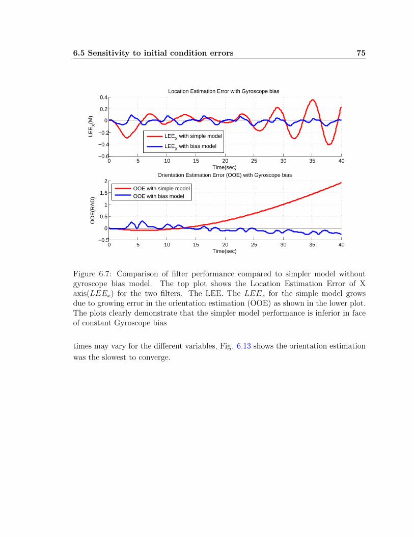
6.5 Sensitivity to initial condition errors 75
0 5 10 15 20 25 30 35 40−0.6
−0.4
−0.2
0
0.2
0.4
Time(sec)
LEE
X(M
)Location Estimation Error with Gyroscope bias
LEEX with simple model
LEEX with bias model
0 5 10 15 20 25 30 35 40−0.5
0
0.5
1
1.5
2
Time(sec)
OO
E(R
AD
)
Orientation Estimation Error (OOE) with Gyroscope bias
OOE with simple modelOOE with bias model
Figure 6.7: Comparison of filter performance compared to simpler model withoutgyroscope bias model. The top plot shows the Location Estimation Error of Xaxis(LEEx) for the two filters. The LEE. The LEEx for the simple model growsdue to growing error in the orientation estimation (OOE) as shown in the lower plot.The plots clearly demonstrate that the simpler model performance is inferior in faceof constant Gyroscope bias
times may vary for the different variables, Fig. 6.13 shows the orientation estimation
was the slowest to converge.

76 Results
0 5 10 15 20 25 30 35
−0.2
−0.1
0
0.1
0.2
0.3
Time(sec)
Rad
Gyro bias compensation during a static period
Estimated biasReal velocity(as reference)Real bias
Figure 6.8: Gyroscope bias tracking during an experiment starting from a staticposition. The bias cannot be determined during the initial static period, it is correctedonly on the 8th second when movement starts. Note the velocity trace is plotted onlyfor reference of movement time, y-axis units are not relevant.
0 5 10 15 20 25 30 35−0.05
0
0.05
0.1
0.15
0.2
0.25
Time(sec)
Rad
Gyroscope bias compensation for differnet bias noise values
Bias noise =1Bias noise =0.3Bias noise =0.08Bias noise =0.02Real gyroscope bias
Figure 6.9: Comparison of filter tracking changing bias for different values of Qwg
[defined in 3.7]. Setting a small value, causes slow divergence

6.5 Sensitivity to initial condition errors 77
0 5 10 15 20 25 30 35 40−0.05
0
0.05
0.1
0.15
0.2
Time(sec)
Acc
eler
atio
n B
ias
(M/S
2 )
Accelerometer bias drift compensation
Real bias − XReal bias − YEstimated bias − XEstimated bias − Y
Figure 6.10: Accelerometer bias tracking. Estimated accelerometer bias values areplotted compared to the real values. The filter converges to the correct bias valuesfor both X and Y axis.
0 5 10 15 20 25 30−1
−0.5
0
0.5
1
1.5
2
Time(sec)
X(M
)
Location estimation with wrong initial locations
Real locationEstimated X. Initial value = 0.5 MEstimated X. Initial value = 1 MEstimated X. Initial value = 1.5 M
Figure 6.11: Location estimation for the X axis with wrong initial conditions. Theplots show wrong initial X values of 0.5 M, 1 M and 1.5 M. The different traces showthe filter converges after at most 20 seconds even for large errors.

78 Results
5 10 15 20 25 30
−2
−1
0
1
2
Time(sec)
Vx(M
/S)
Velocity Estimation with wrong initial velocity
Real velocityEstimated Vx. Initial value = 1 M/S
Estimated Vx. Initial value = 2 M/S
Estimated Vx. Initial value = −1 M/S
Estimated Vx. Initial value = −2 M/S
Figure 6.12: Velocity estimation for the X axis with wrong initial conditions. Theplots show wrong initial X values of 1 M/S, 2 M/S, -1 M/S and -2 M/S. The differenttraces show the filter converges after at most 25 seconds even for large errors.
0 10 20 30 40 50 60 70−4
−3
−2
−1
0
1
2
3
Time(sec)
Rot
atio
n(R
AD
)
Orientation Estimation error with wrong initial rotation
Real orientationEstimated orientation. Initial angle = −2 RADEstimated orientation. Initial angle = −1 RADEstimated orientation. Initial angle = 1 RAD
Figure 6.13: Orientation estimation error. Orientation is represented as a counterclock-wise rotation in the XY plane. The plots show wrong initial values of 1 RAD,2 RAD, -1 RAD and -2 RAD. For large errors, the convergence occurs only afterconsiderable time.

Chapter 7
Discussion and Future Work
The filter parameter initialization reported in Table 6.1 is found to work well after
running an extensive number of tests in the presence of the simulated disturbances.
Of course, for different trajectories and time-varying disturbances, different sets of
filter parameters would be better. The discussion in Section 6.3 outlines the major
implications on overall filter performance caused by setting an inappropriate gyro-
scope bias instability value. The same treatment can be done to the other 15 variables
in the kalman state vector, hence finding the optimal filter parameters is an intricate
and constant task. Not only sensor noise parameters are taken into considerations,
but also the shape of the path and velocity of the movement (which affect RSSI bias
modeling), even SHIMMER’s battery depletion might increase the bias instability
factor.
The proposed filter outperforms the RSSI-based system but not significantly. This
is due to a number of reasons :
• The Root Mean Square criterion does not tell the whole story. As shown in
Figure 6.4, the filter tracks the movement pattern and shape much better then
the RSSI-based algorithm, a different criterion might reward this behavior more
significantly.
• The use of noisy and bias unstable sensors in the real-world experiments. As
Figure 6.1 shows, that SHIMMER sensors suffer from severe bias drift which
degrades filter performance. In future work, these experiments will be repeated
with the newer generation sensors, e.g. SHIMMER2, possibly integrating the
inertial sensors with more drift-free sensors such as magnetometers. Simulation
results using improved inertial sensors achieve far better results, as seen in this

80 Discussion and Future Work
table 7.1 compared to the initial table 6.2.
• RSSI-based estimations errors are slow changing and are not optimally modeled
with a gaussian white noise process as the kalman filter requires. A possible
solution, is to further investigate in the future other types of filters, such as the
particle filter which are more capable with handling such errors.
• Sampling rate considerations are not taken into account. Any real-world system
will restrict the RSSI sampling rate due to energy consumption considerations.
Lower sampling rates will greatly degrade the RSSI-based estimation accuracy,
becoming more dependent of the successful fusion with inertial sensors. Fu-
ture work will investigate the filter performance under different sampling rates
constraints.
There are a number of ways the current sensor setup can be improved. First,
incorporating newer inertial sensors such as the SHIMMER2 motes and integrating
them with aiding sensors such as magnometers will greatly improve results [28]. Sec-
ond, the presented kalman filter successfully combines inertial data with RSSI-based
estimations, but handles each system in a black box manner. Borrowing terms from
the GPS/INS world, the presented filter is a closed-loop design with no feedback
[81]. The future work will be addressed to apply the ideas presented here with an
open-loop design, using the RSSI bias estimation as a feedback to the RSSI-based
estimator. As in the realm of GPS/INS, where open-loop designs allow for intimate
cooperation between the systems, it applies here too. The RSSI-based system can
use the information to detect in real-time shadowing effects and learn how to better
compensate for them.
Although the prototype system works under lab conditions, the path to a useful
tracking system for Body Sensor Networks is long and hard. Lets review some of the
major milestones left for future research:
From 2D to 3D The RSSI-based system is currently only implemented in 2D. De-
veloping the system to work with more anchor nodes and supply 3D estimations
is critical.
BSN implementation The system should be able to run in real-time on-board the
moving object. This requires implementing the whole system on a single wireless
mote, including hardware (current setup uses two different platforms for INS
and RSSI) and software (code in TinyOs and not matlab).

81
Dynamic anchor nodes RSSI-based algorithms assume the anchor nodes are static,
whereas in the realm of human motion tracking, the body moves and so the an-
chor nodes move too. This has two major implications, first the RSSI-based
algorithm must be verified to work in a dynamic environment and second the
inertial system must implement algorithms for deferential inertial tracking be-
tween the limbs and the body. The required system is similar to the work
of Foxlin et al. [36] which implemented differential inertial tracking between
helmet-mounted and aircraft-mounted inertial sensors as part of the develop-
ment of FlightTracker, a system for cockpit enhanced vision.
Estimation method Location error RMS (M)
Pure inertial system 3.76 [for 50 seconds experiment]. Unbounded.Pure RSSI-based system 0.058Proposed filter (inertial and RSSI) 0.042
Table 7.1: RMSE values for each estimation method from simulation results

Chapter 8
Conclusions
This thesis presents the design, implementation, simulations and real-world exper-
imental results of a sensor-fusion Kalman filter for real-time human body motion
tracking using inertial/RSSI sensors. The complete design of the filter was pre-
sented,detailing the inner workings of each sub system and the full derivation of
the complementary kalman filter used for sensor fusion. Also, a new and simple
derivation for the orientation estimation kalman filter based on Luinge et at. work
[43] was presented (see Section 4.1.2). A real-world experimental setup was built,
including a state-of-the-art optical tracking device used as reference. Finally, real-
world experiments of hand movement were performed but only in a controlled, 2D
environment and with a custom made RSSI-based setup. Implementation of the filter
on existing BSNs with full human motion testing in real-life environment is left for
future research.
The Kalman filter design presented in this work is the result of two years of effort
into close-proximity RSSI-based tracking systems. Continuing the work of Blumrozen
et al. in [56] and [16], this research expands their work to the realm of Inertial
Body Sensor Networks. Although this system is merely an oversimplified prototype
(as discussed in Section 7), this filter holds great potential to be implemented by
numerous existing and future Body Sensor Networks (BSNs) with inertial sensors
and wireless capability, as aiding the tracking algorithm with RSSI data comes with
no added hardware costs.

Bibliography
[1] Eric Foxlin. Chapter 7 . motion tracking requirements and technologies. Envi-
ronment, pages 163–210, 2002.
[2] Benny P. L. Lo and Guang-Zhong Yang. Key Technical Challenges and Cur-
rent Implementations of Body Sensor Networks. In International Workshop on
Wearable and Implantable Body Sensor Networks, April 2005.
[3] B.R.; McGrath M.J.; O’Shea T.J.; Kuris B.; Ayer S.M.; Stroiescu F.; Cionca V.
Burns, A.; Greene. Shimmer a wireless sensor platform for noninvasive biomed-
ical research. In Sensors Journal, IEEE, September 2010.
[4] K Tong and M H Granat. A practical gait analysis system using gyroscopes.
Medical Engineering and Physics, 21(2):87–94, 1999.
[5] Kamiar Aminian, B Najafi, C Bla, P-F Leyvraz, and Ph Robert. Spatio-temporal
parameters of gait measured by an ambulatory system using miniature gyro-
scopes. Journal of Biomechanics, 35(5):689–699, 2002.
[6] R Williamson and B J Andrews. Sensor systems for lower limb functional elec-
trical stimulation (fes) control. Medical Engineering and Physics, 22(5):313–25,
2000.
[7] K Y Tong and M H Granat. Virtual artificial sensor technique for functional
electrical stimulation. Medical Engineering and Physics, 20(6):458–468, 1998.
[8] P H Veltink, P Slycke, J Hemssems, R Buschman, G Bultstra, and H Hermens.
Three dimensional inertial sensing of foot movements for automatic tuning of a
two-channel implantable drop-foot stimulator. Medical Engineering and Physics,
25(1):21–28, 2003.

84 Bibliography
[9] A T Willemsen, F Bloemhof, and H B Boom. Automatic stance-swing phase
detection from accelerometer data for peroneal nerve stimulation. IEEE Trans-
actions on Biomedical Engineering, 37(12):1201–1208, 1990.
[10] M J Mathie, A C F Coster, N H Lovell, and B G Celler. Detection of daily phys-
ical activities using a triaxial accelerometer. Medical and Biological Engineering
and Computing, 41(3):296–301, 2003.
[11] F Foerster. Detection of posture and motion by accelerometry: a validation study
in ambulatory monitoring. Computers in Human Behavior, 15(5):571–583, 1999.
[12] Carlijn V C Bouten, Karel T M Koekkoek, Maarten Verduin, Rens Kodde, and
Jan D Janssen. A triaxial accelerometer and portable data processing unit for
the assessment of daily physical activity. IEEE Transactions on Biomedical En-
gineering, 44(3):136–147, 1997.
[13] Am Sabatini. Inertial sensing in biomechanics: a survey of computational tech-
niques bridging motion analysis and personal navigation, volume 1, page 70100.
Idea Group Pubilishing: Hershey, PA, USA, 2006.
[14] N Yazdi, F Ayazi, and K Najafi. Micromachined inertial sensors. Proceedings of
the IEEE, 86(8):1640–1659, 1998.
[15] Xiaoping Yun, Eric R Bachmann, Hyatt Moore, and James Calusdian. Self-
contained position tracking of human movement using small inertial/magnetic
sensor modules. Proceedings 2007 IEEE International Conference on Robotics
and Automation, (April):2526–2533, 2007.
[16] Tal Anker Danny Dolev Boris Rubinsky Gaddi Blumrozen, Bracha Hod. En-
hancing rssi-based tracking accuracy in wireless sensor networks. To be published
on ACM Transactions on Sensor Networks, 2011.
[17] N Yazdi, F Ayazi, and K Najafi. Micromachined inertial sensors. Proceedings of
the IEEE, 86(8):1640–1659, 1998.
[18] XSens. Xsens mtx inertial sensor, 2011.
[19] Jawbone Inc. Wireless wristband for a healthier life. http://http://jawbone.
com/up, 2011. [Online; accessed 1-December-2011].
Bibliography 85
[20] H Zhou and H Hu. Human motion tracking for rehabilitationa survey. Biomedical
Signal Processing And Control, 3(1):1–18, 2008.
[21] Inertial Navigation. Inertial navigation forty years of evolution. Evolution,
13(3):140–149, 1998.
[22] M F Golnaraghi. A vector-based gyro-free inertial navigation system by integrat-
ing existing accelerometer network in a passenger vehicle. PLANS 2004 Position
Location and Navigation Symposium IEEE Cat No04CH37556, pages 234–242,
2004.
[23] B Barshan and H F Durrant-Whyte. Inertial navigation systems for mobile
robots. IEEE Transactions on Robotics and Automation, 11(3):328–342, 1995.
[24] Suya You, Ulrich Neumann, and Ronald Azuma. Hybrid inertial and vision
tracking for augmented reality registration, volume 19, pages 260–267. IEEE,
1999.
[25] Greg Welch. Motion tracking : No silver bullet , but a respectable. IEEE
Computer Graphics and Applications, (December), 2002.
[26] Oliver J. Woodman, C Oliver J. Woodman, and Oliver J. Woodman. An intro-
duction to inertial navigation, 2007.
[27] Benoit Huyghe, Jan Doutreloigne, and Jan Vanfleteren. 3d orientation tracking
based on unscented kalman filtering of accelerometer and magnetometer data.
2009 IEEE Sensors Applications Symposium, (1):148–152, 2009.
[28] Eric Robert Bachmann. Inertial and magnetic tracking of limb segment orien-
tation for inserting humans into synthetic environments. PhD thesis, Citeseer,
2000.
[29] D Roetenberg, H Luinge, and P Veltink. Inertial and magnetic sensing of human
movement near ferromagnetic materials. The Second IEEE and ACM Inter-
national Symposium on Mixed and Augmented Reality 2003 Proceedings, pages
268–269, 2006.
[30] Y Tao, H Hu, and H Zhou. Integration of vision and inertial sensors for 3d
arm motion tracking in home-based rehabilitation. The International Journal of
Robotics Research, 26(6):607–624, 2007.

86 Bibliography
[31] J A Corrales, F A Candelas, and F Torres. Hybrid tracking of human operators
using imu/uwb data fusion by a kalman filter. Proceedings of the 3rd international
conference on Human robot interaction HRI 08, page 193, 2008.
[32] L. Sher. Personal inertial navigation system (pins). 1996.
[33] Daniel Vlasic, Rolf Adelsberger, Giovanni Vannucci, John Barnwell, Markus
Gross, Wojciech Matusik, and Jovan Popovic. Practical motion capture in ev-
eryday surroundings. ACM Transactions on Graphics, 26(3):35, 2007.
[34] P Corke, J Lobo, and J Dias. An introduction to inertial and visual sensing. The
International Journal of Robotics Research, 26(6):519–535, 2007.
[35] Eric Foxlin and Leonid Naimark. VIS-Tracker: A Wearable Vision-Inertial Self-
Tracker. 2003.
[36] Eric Foxlin, Yury Altshuler, Leonid Naimark, and Mike Harrington. Flighttracker
: A novel optical / inertial tracker for cockpit enhanced vision. Third IEEE and
ACM International Symposium on Mixed and Augmented Reality, (Ismar):212–
221, 2004.
[37] J Lobo and J Dias. Vision and inertial sensor cooperation using gravity as a verti-
cal reference. IEEE Transactions on Pattern Analysis and Machine Intelligence,
25(12):1597–1608, 2003.
[38] Toshiharu Mukai and Noboru Ohnishi. The recovery of object shape and camera
motion using a sensing system with a video camera and a gyro sensor. Proceedings
of the Seventh IEEE International Conference on Computer Vision, 1(1):411–417
vol.1, 1999.
[39] Francesco Panerai, Giorgio Metta, and Giulio Sandini. Visuo-inertial stabiliza-
tion in space-variant binocular systems. Robotics and Autonomous Systems,
30(1-2):195–214, 2000.
[40] E Foxlin. Inertial head-tracker sensor fusion by a complementary separate-bias
kalman filter. Proceedings of the IEEE 1996 Virtual Reality Annual International
Symposium, 96:185–194,, 1996.
[41] Eric Foxlin. Pedestrian tracking with shoe-mounted inertial sensors. IEEE Com-
puter Graphics and Applications, 25(6):38–46, 2005.

Bibliography 87
[42] Xiaoping Yun, Eric R Bachmann, Hyatt Moore, and James Calusdian. Self-
contained position tracking of human movement using small inertial/magnetic
sensor modules. Proceedings 2007 IEEE International Conference on Robotics
and Automation, (April):2526–2533, 2007.
[43] H J Luinge and P H Veltink. Measuring orientation of human body segments us-
ing miniature gyroscopes and accelerometers. Medical and Biological Engineering
and Computing, 43(2):273–282, 2005.
[44] Xiaoping Yun and Eric R Bachmann. Design, implementation, and experimental
results of a quaternion-based kalman filter for human body motion tracking.
IEEE Transactions on Robotics, 22(6):1216–1227, 2006.
[45] A D Young. Use of body model constraints to improve accuracy of inertial
motion capture. 2010 International Conference on Body Sensor Networks, pages
180–186, 2010.
[46] Huiyu Zhou, Huosheng Hu, and A Motivation. Kinematic model aided inertial
motion tracking of human upper limb. 2005 IEEE International Conference on
Information Acquisition, pages 150–155, 2005.
[47] Ferial Shayeganfar, Amin Anjomshoaa, and A Min Tjoa. A smart indoor naviga-
tion solution based on building information model and google android. Method-
ology, 5105:1050–1056, 2008.
[48] Hui Liu, Houshang Darabi, Pat Banerjee, and Jing Liu. Survey of wireless
indoor positioning techniques and systems. IEEE Transactions on Systems Man
and Cybernetics Part C Applications and Reviews, 37(6):1067–1080, 2007.
[49] Localization of wireless sensor networks with a mobile beacon. 2004 IEEE
International Conference on Mobile Adhoc and Sensor Systems IEEE Cat
No04EX975, (July).
[50] Tsenka Stoyanova, Fotis Kerasiotis, Aggeliki Prayati, and George Papadopou-
los. Evaluation of impact factors on rss accuracy for localization and tracking
applications. Proceedings of the 5th ACM international workshop on Mobility
management and wireless access MobiWac 07, Im(17):9, 2007.

88 Bibliography
[51] F V F De Lima and C M Furukawa. Development and testing of an acoustic
positioning system - description and signal processing, volume 1, pages 849 – 852
vol.1. 2002.
[52] Andreas Savvides, Heemin Park, and Mani B Srivastava. The bits and flops of the
n-hop multilateration primitive for node localization problems. Proceedings of the
1st ACM international workshop on Wireless sensor networks and applications
WSNA 02, pages 112–121, 2002.
[53] Andreas Savvides, Heemin Park, and Mani B Srivastava. The n-hop multilatera-
tion primitive for node localization problems. Mobile Networks and Applications,
pages 443–451, 2003.
[54] P Bahl and V N Padmanabhan. Radar: an in-building rf-based user location and
tracking system. Proceedings IEEE INFOCOM 2000 Conference on Computer
Communications Nineteenth Annual Joint Conference of the IEEE Computer
and Communications Societies Cat No00CH37064, 2(c):775–784, 2000.
[55] Mohit Saxena, Puneet Gupta, and Bijendra Nath Jain. Experimental analysis
of rssi-based location estimation in wireless sensor networks. 2008 3rd Inter-
national Conference on Communication Systems Software and Middleware and
Workshops COMSWARE 08, pages 503–510, 2008.
[56] Gaddi Blumrosen, Bracha Hod, Tal Anker, Danny Dolev, and Boris Rubinsky.
Continuous close-proximity rssi-based tracking in wireless sensor networks. In
BSN, pages 234–239, 2010.
[57] Lasse Klingbeil, Richard Reiner, Michailas Romanovas, Martin Traechtler, and
Yiannos Manoli. Multi-modal sensor data and information fusion for localization
in indoor environments. Spectrum, pages 187–192, 2010.
[58] Andreas Fink, Helmut Beikirch, Matthias Vo?, and Christian Schr. RSSI-based
Indoor Positioning using Diversity and Inertial Navigation, pages 15–17. Number
September. 2010.
[59] Fr?d?ric Evennou and Fran?ois Marx. Advanced integration of wifi and iner-
tial navigation systems for indoor mobile positioning. EURASIP Journal on
Advances in Signal Processing, 2006:1–12.

Bibliography 89
[60] John Bortz. A new mathematical formulation for strapdown inertial navigation.
Ieee Transactions On Aerospace And Electronic Systems, AES-7(1):61–66, 1971.
[61] M S Grewal, L R Weill, and A P Andrews. Global positioning systems, inertial
navigation, and integration, page 364. Wiley-Interscience, 2007.
[62] Robert Grover Brown and Patrick Y C Hwang. Introduction to Random Signals
and Applied Kalman Filtering, volume 2, page 401. John Wiley and Sons, 1997.
[63] G Mao, B Fidan, and B Anderson. Wireless sensor network localization tech-
niques. Computer Networks, 51(10):2529–2553, 2007.
[64] Eli Brookner. Tracking and Kalman Filtering Made Easy, volume 1, page 107.
John Wiley and Sons, Inc., 1998.
[65] Robert Grover Brown and Patrick Y C Hwang. Introduction to Random Signals
and Applied Kalman Filtering, volume 2, page 195. John Wiley and Sons, 1997.
[66] Dan Simon. Optimal State Estimation, volume 2, page 26. John Wiley and Sons,
Inc., 2006.
[67] Dan Simon. Optimal State Estimation, volume 2, page 189. John Wiley and
Sons, Inc., 2006.
[68] Peter Henrici. Introduction to applied mathematics (gilbert strang). SIAM
Review, 28(4):590, 1986.
[69] Robert Grover Brown and Patrick Y C Hwang. Introduction to Random Signals
and Applied Kalman Filtering, volume 2, page 392. John Wiley and Sons, 1997.
[70] K Pahlavan and J P Makela. Indoor geolocation science and technology. IEEE
Communications Magazine, 40(2):112–118, 2002.
[71] S Hara, K Yanagihara, J Taketsugu, K Fukui, S Fukunaga, and K Kitayama.
Propagation characteristics of ieee 802.15.4 radio signal and their application for
location estimation. 2005 IEEE 61st Vehicular Technology Conference, 1(c):97–
101, 2005.
[72] W. LIAO and Y LEE. A lightweight localization scheme in wireless sensor net-
works. ICWMC06, 2006.

90 Bibliography
[73] Dan Simon. Optimal State Estimation, volume 2, page 19. John Wiley and Sons,
Inc., 2006.
[74] S. E. Leis. Ndi-tb-0005: Polaris calibration performance and methodology, rev.
002. tech. rep. Northern Digital Inc., 1996.
[75] Intel Corporation. The shimmer sensor node platform. 2006. [Online]. Available:
http://www.eecs.harvard.edu/ mdw/proj/codeblu.
[76] B. Lo, S. Thiemjarus, R. King, and G.Z. Yang. Body sensor network–a wireless
sensor platform for pervasive healthcare monitoring. In The 3rd International
Conference on Pervasive Computing, volume 13. Citeseer, 2005.
[77] AS Chipcon. CC2420 2.4 GHz IEEE 802.15. 4/ZigBee-ready RF Transceiver.
Chipcon AS, Oslo, Norway, 4, 2004.
[78] Sohan Ranjana Brian Blakec Kevin Clearya, Luis Ibanezb. Igstk: a software
toolkit for image-guided surgery applications. Computer Aided Radiology and
Surgery, 2004.
[79] Oliver J. Woodman. An introduction to inertial navigation. 2007.
[80] Standard specification format guide and test procedure for single-axis interfero-
metric fiber optic gyros. IEEE Std 962, 2003.
[81] R T Kelley, I N Katz, and C A Bedoya. Design, development and evaluation of
an Ada coded INS/GPS open loop Kalman filter, volume 4, page 382388. IEEE,
1990.