V MODELLING WEEK

Complutense University of Madrid

Faculty of Mathematical Sciences

Estimation of Orientation

Distribution of Fibers

Authors:

Davidovic A.

Gargallo-Peiro A.

Llontop Garcıa M.

Munoz Ortega F.J.

Toledo Carrasco D.

Wang C.

Advisor:

Dr. Jouni Sampo1

MadridJune 21, 2011

1Lappeeranta University of Technology, Finland

Contents

1 Introduction and motivation 3

2 Structure tensor technique 4

2.1 Theoretical basis . . . . . . . . . . . . . . . . . . . . . . . . . 4

2.2 Results . . . . . . . . . . . . . . . . . . . . . . . . . . . . . . . 6

2.3 New weight strategy: an attempt to improve the method . . . 9

3 Fast Fourier Transform Method 12

3.1 Numerical calculation of fiber distribution . . . . . . . . . . . 12

3.2 Results . . . . . . . . . . . . . . . . . . . . . . . . . . . . . . . 13

4 Conclusions 16

A Imaged paper sheets and image processing 17

A.1 Images of fiber distribution of several paper sheets . . . . . . . 17

A.1.1 Fiber distributions of simulated paper sheets . . . . . . 17

A.1.2 Fiber distributions of real paper sheets . . . . . . . . . 18

A.2 Image Processing . . . . . . . . . . . . . . . . . . . . . . . . . 18

A.2.1 Smoothing Operations . . . . . . . . . . . . . . . . . . 19

A.2.2 Rolling Ball algorithm for subtract background . . . . 19

A.2.3 Thresholding . . . . . . . . . . . . . . . . . . . . . . . 19

A.2.4 Results of the processing . . . . . . . . . . . . . . . . . 20

1 Introduction and motivation

Paper is composed mainly by wood fibers and mineral fillers, together withother additives that conform the basic structure of the sheet. The distribu-tion of the fibers that compose the paper determines its properties. Then,it is of the major importance in the paper production industry to be able toproperly analyse the distribution properties in order to ensure a good qualitypaper.

It is in this context where the presented work is placed. In this framework,in order to ensure that the produced paper ensures a certain distribution offibers (or either ensures that the fibers do not configure a certain criticaldistribution), the related industries require techniques that estimate the ori-entation distribution of the produced paper sheets.

Such techniques must be able to, given a certain image of a paper sheetwhere there can be distinguished the inner fibers, determine the orientationdistribution of such set of fibers.

The objective of this project is to study and analyse two specific tech-niques: a Structure Tensor based method, and a Fast Transform Fouriertechnique. Once programmed and analysed the limitations and strong pointsof such methods, new ideas will be tried to be introduced in order to improvetheir performance.

Several imaging techniques can be used in order to analyse the papersheets. In these project we have used the following main set of image types:

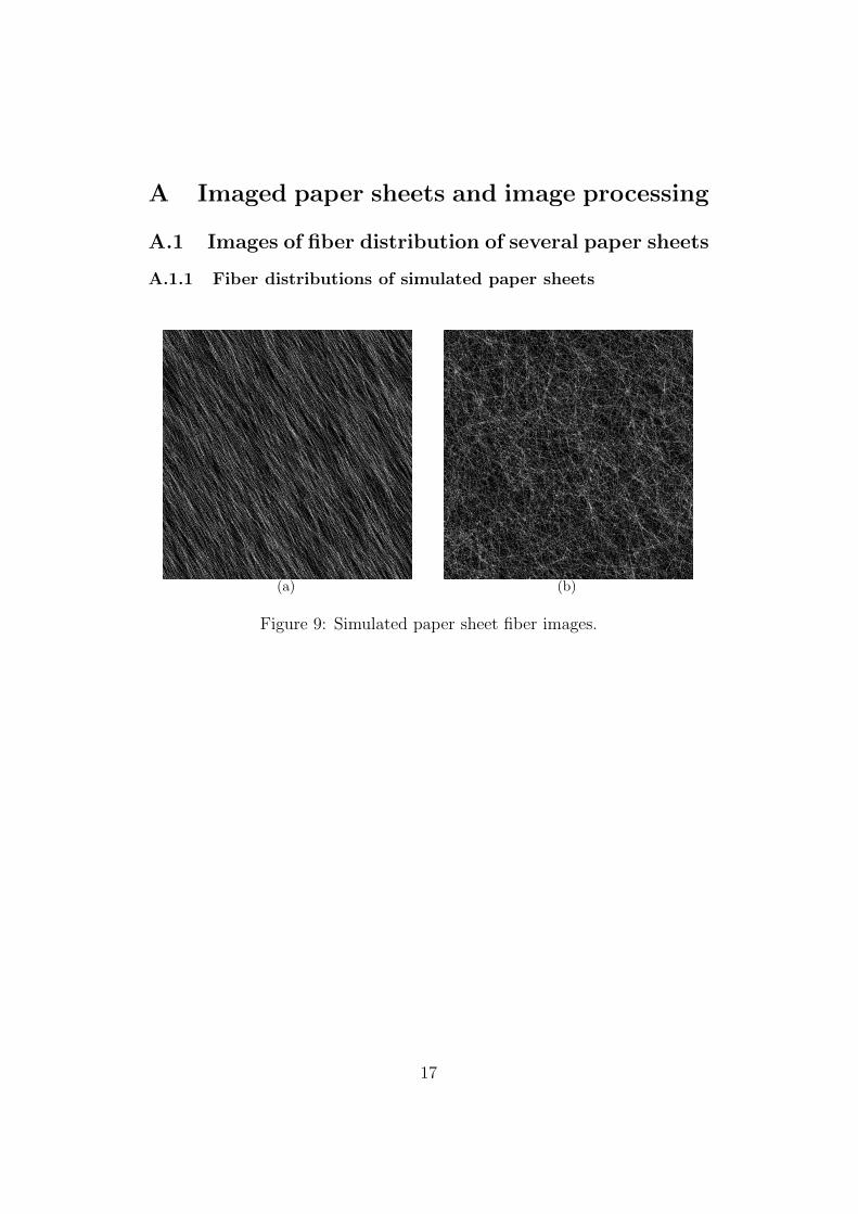
• Simulated fiber distribution that are represent microscope type-images,see Figure 9.

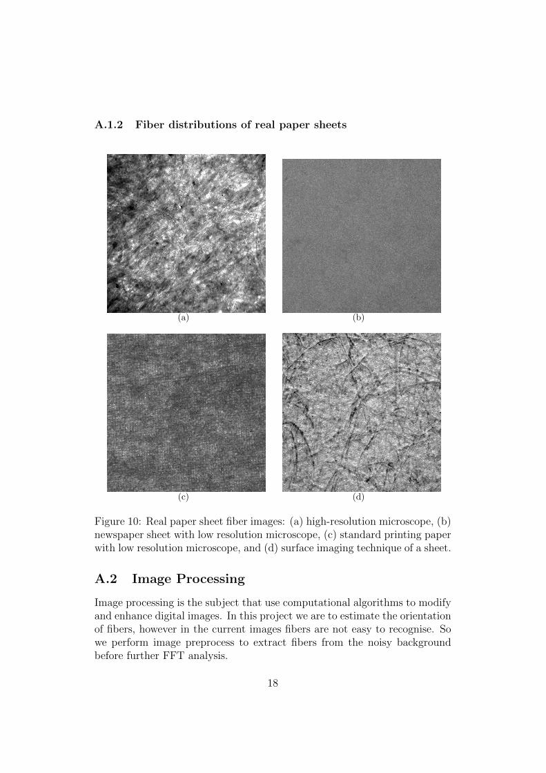
• Real fiber distributions of paper sheets taken with surface imaging tech-nique (different incident lights on the surface of the paper), see Figure10(d).

• Real fiber distributions of paper sheets taken with low quality imagingwith microscopes, see Figures 10(b) and 10(c).

• Real fiber distribution of paper sheets taken with high quality resolu-tion with electronic microscopes 3(a).

Moreover note that Figure 10(c) corresponds to a newspaper sheet ofpaper, and that the rest of not simulated images correspond to differentstandard printing paper sheets.

3

2 Structure tensor technique

2.1 Theoretical basis

The basic idea of the method is to observe a small part of the image, calledwindow and obtain average orientation of the fibers in it. For obtainingdistribution of the orientation on all image we slide window along image ob-taining different values depending on which part of the image we observe ateach time. As we will see distributions will highly depend on the size of thewindow we use and on the step that we take for moving window along theimage.The windows are defined as a function on the image domain that is zero val-ued outside the subdomain of interest and weights under a certain criteria.In our case, window is a square that is determined with central point (x0, y0)and the length of the square side L.Let us now explain how to compute average orientation of the fibers in thegiven window. Consider the weighted inner product of two R2 valued func-tions f and g,

〈f, g〉w =

∫ ∫R2

w(x, y)f(x, y)g(x, y)dxdy, (2.1)

where w(x, y) ≥ 0 is a weight function. The simple example of the weightfunction is the identity weight given as w(x, y) = 1 for points inside of thewindow and 0 elsewhere. The norm of f is defined by ‖f‖ =

√〈f, f〉w. In

our case f is a function of intensity of grey color, i.e. f = 0 for white pixelsand f = 255 for black pixels. Areas with less fibers in the image will bedarker. Also if the fibers are mostly oriented in one specific direction, therewill be more variation in intensity of grey in normal direction to that one.Hence, we are interested in directional derivative of the function f given by

Duθf(x, y) = uTθ∇f(x, y)

where ∇f(x, y) = (fx, fy) is the gradient of f and uθ = (cos θ, sin θ) is a unitvector that gives direction. The directional derivative gives a measure of thechange of the color in a given direction. We are interested in the directionwhere this change is maximized, and we will compute it for each window. Itis given by

u = arg max‖uθ‖=1

‖Duθf(x, y)‖2w.

The structure tensor of f is 2× 2 matrix defined as

J =⟨∇f,∇fT

⟩w

=

[〈fx, fx〉w 〈fx, fy〉w〈fx, fy〉w 〈fy, fy〉w

]. (2.2)

4

Now we can write

‖Duθf(x, y)‖2w =⟨uTθ∇f,∇fTuθ

⟩= uTθ Juθ.

The Lagrange function of the optimisation problem is

Λ(uθ, λ) = uTθ Juθ + λ(uTθ uθ − 1

).

Then, setting the derivative of Λ w.r.t. uθ equal to 0 we get that solution ofthe optimisation problem satisfies

Ju = λu. (2.3)

Hence, the directional derivative is maximized in the direction of the eigenvec-tor that corresponds to maximal eigenvalue of J , λmax = max ‖Duθf(x, y)‖2w,and minimized in orthogonal direction given by the second eigenvector andλmin = min ‖Duθf(x, y)‖2w. The eigenvalues of J are

λ1,2 = 〈fx, fx〉w + 〈fy, fy〉w ±√

(〈fx, fx〉w − 〈fy, fy〉w)2 + 4 〈fx, fy〉2w

Substituting these values in (2.3) and keeping in mind uθ = (cos θ, sin θ) weobtain that the peak of the distribution is given as

θ =1

2arctan

(2 〈fx, fy〉w

〈fy, fy〉w − 〈fx, fx〉w

). (2.4)

There are some improvements that can be done using some additional infor-mation that can be extracted directly from the structure tensor. The firstone is coherency, given by

C =λmax − λmin

λmax + λmin

=

√(〈fy, fy〉w − 〈fx, fx〉w

)2+ 4 〈fx, fy〉2w

〈fy, fy〉w + 〈fx, fx〉w∈ [0, 1]. (2.5)

If in the window there is one dominant orientation, the coherency will be near1. On the other hand if in the window coherency is close to 0 it means thatfibers are almost uniformly distributed in each direction. In this case windowdoes not give good information, and we can disregard information obtainedfrom this window. The second improvement can be done using energy, givenby

E = Trace(J). (2.6)

The energy will be higher in the windows where we have more fibers. Hencewe can disregard windows with the low energies.

5

Algorithm 2.1 shows schematically the computational procedure that hasto be brought up in order to compute the structure tensor for the deter-mination of the orientation distribution. We have implemented Algorithm2.1 using Matlab. More information about the structure tensor method forimage analysis can be found on References [1, 2, 3].

Algorithm 2.1 Structure tensor technique algorithm

Ensure: Grey map f .1: function Getθ(f)2: f ← filter f3: p1, . . . , pnp ← set discretization of np points4: L← set window length5: θ, E,C ← allocate angle, energy and coherency vectors of size np6: for k = 1 : np do7: pk ← fix point k of the discretization8: Wk ← set window domain of edge length L and weights9: Jk ← compute structure tensor matrix (see Equation (2.2))

10: θ(k), E(k), C(k)← compute parameters (see (2.4), (2.5), (2.6))11: end for12: end function

2.2 Results

In this section we present the results corresponding to the structure tensortechnique for the paper sheets shown in Figures 9 and 10, corresponding todistribution of fibers of simulated and real papers.

For each analysed fiber distribution we present an image with the re-sults obtained using the structure tensor with different window sizes anddiscretizations. We specifically have selected to present three types of win-dows. A wide window (compared to the width of the image domain) in acoarse distribution of points, a midsize window in a refined distribution, anda really narrow window in a dense distribution of points. For all windows,the weighting function is considered as the identity inside the window (andtaking zero value outside of it).

Figure 1(a) shows the orientation distribution of the fibers correspondingto Figure 9(a). The x-axis, [0, 180] degrees, corresponds to the angle orien-tations of the fibers. The y-axis corresponds to the ”number” of fibers withthe corresponding orientation. The analysed image, Figure 9(a), correspondsto a simulated paper sheet, created using a low randomized pattern of theorientation of the fibers. The fiber distribution in red corresponds to the

6

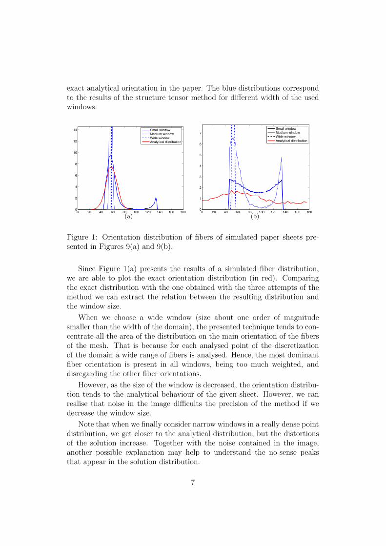
exact analytical orientation in the paper. The blue distributions correspondto the results of the structure tensor method for different width of the usedwindows.

0 20 40 60 80 100 120 140 160 1800

2

4

6

8

10

12

14

Small window

Medium window

Wide window

Analytical distribution

(a)0 20 40 60 80 100 120 140 160 180

0

1

2

3

4

5

6

7

Small window

Medium window

Wide window

Analytical distribution

(b)

Figure 1: Orientation distribution of fibers of simulated paper sheets pre-sented in Figures 9(a) and 9(b).

Since Figure 1(a) presents the results of a simulated fiber distribution,we are able to plot the exact orientation distribution (in red). Comparingthe exact distribution with the one obtained with the three attempts of themethod we can extract the relation between the resulting distribution andthe window size.

When we choose a wide window (size about one order of magnitudesmaller than the width of the domain), the presented technique tends to con-centrate all the area of the distribution on the main orientation of the fibersof the mesh. That is because for each analysed point of the discretizationof the domain a wide range of fibers is analysed. Hence, the most dominantfiber orientation is present in all windows, being too much weighted, anddisregarding the other fiber orientations.

However, as the size of the window is decreased, the orientation distribu-tion tends to the analytical behaviour of the given sheet. However, we canrealise that noise in the image difficults the precision of the method if wedecrease the window size.

Note that when we finally consider narrow windows in a really dense pointdistribution, we get closer to the analytical distribution, but the distortionsof the solution increase. Together with the noise contained in the image,another possible explanation may help to understand the no-sense peaksthat appear in the solution distribution.

7

Figure 2: Problematic originated due to the use of narrow windows.

Figure 2 presents an scheme of the added problems that appear due tothe use of narrow windows in the analysis. Imagine that a narrow windowis opened at the end of one fiber. The arrows that appear in 2 representthe gradients of the function on the boundary of the fiber. If we then con-sider the orientation in such window using the structure tensor, the presentedtechnique may not distinguish between the edge of the fiber, and its width.Hence, in such window we would extract that there are two main orienta-tions: the orientation of the fiber, and another one about 90◦ translatedcorresponding to its cross-section. Note that the cross-section gradient is afalse orientation angle, and hence, this introduces an error in the solution.

Looking at the results for this first simple image 1(a), we realize thatthe presented method is going to become a really useful and robust key todetermine the main fiber orientation in a paper. However, we have observedan important perturbation when the behaviour of the analytical solutionis trying to being approximated by reducing the window size. From thisoscillations we realize that the method is really sensitive to noise of thepaper image.

Results presented in Figure 3 show the orientation distribution of morecomplex fiber distributions. All the presented results correspond to real papersheet distributions, see Figure 10.

Note that in Figure 3(a), the estimation of the orientation distributionis far from being precise. When the structure tensor is created using a widewindow, we can clearly see that we are able to catch properly the mainorientation of the fibers, but oscillations appear. However, when we decreasethe window width, quite a different pattern, with almost no characteristicorientation can be found. Recall that the same commentaries apply to 3(b)and 3(d). Figure 3(c) seems to be a bit stable, although we have no way tototally confirm the given results.

8

0 20 40 60 80 100 120 140 160 1800

1

2

3

4

5

6

7

Small window

Medium window

Wide window

(a)0 20 40 60 80 100 120 140 160 180

0

1

2

3

4

5

6

7

Small window

Medium window

Wide window

(b)

0 20 40 60 80 100 120 140 160 1800

1

2

3

4

5

6

7

Small window

Medium window

Wide window

(c)0 20 40 60 80 100 120 140 160 180

0

1

2

3

4

5

6

7

Small window

Medium window

Wide window

(d)

Figure 3: Orientation distribution of fibers of real paper sheets presented in(a) Figure 10(a), (b) Figure 10(b), (c) Figure 10(c), and (d) Figure 10(d).

2.3 New weight strategy: an attempt to improve themethod

From the results presented in Section 2.2 we realise that the structure tensormethod is limited when we want to use it to determine the exact orientationdistribution of the fibers in a paper. However, is worth it remarking that itis a precise method to detect the main orientation of the fibers of the papersheet.

In an attempt to improve the way that the method considers the orien-tation distribution of an opened window, we have defined a new weightingfunction in terms of the energy and the coherency. Fixed a window width,the window function is not any more considered as the identity inside thewindow and zero outside it. Instead of this simple defined function, a dif-ferent weight is assigned to each point. The weight assigned corresponds to

9

a function of the energy and coherency on the nearby region of this point.Such region is going to be considered as a small window that contains justthe closest pixels to the analysed one.

Recall that the coherency is a parameter in the interval [0, 1], taking zerowhen there is no a main orientation in a window, and taking one there is justone orientation in the window. Moreover, the energy is a parameter that cantake a wide range of values, and that is bigger and bigger in relation to thenumber of fibers and changes of gradient in function f (gray scale function).

Hence, if we want to somehow weight a point in function of its importancein the determination of the fiber orientation distribution, we require to useboth parameters. The proposed weight function is defined as

w(x, y) =Csw(x,y) · Esw(x,y)

Emax, (2.7)

where Csw(x,y) and Esw(x,y) denote the coherency and the energy in the sub-window defined on point (x, y), and Emax denotes the maximum energyamong all the subwindows that are considered in the image domain. Hence,note that w(x, y) ∈ [0, 1], taking close to 1 values when the orientation ofthe subwindow is very clear and there is a high fiber presence, and closeto 0 values when either there is no main orientation or there is a low fiberpresence.

0 20 40 60 80 100 120 140 160 1800

2

4

6

8

10

12

14

Small window

Medium window

Wide window

Analytical distribution

(a)0 20 40 60 80 100 120 140 160 180

0

1

2

3

4

5

6

7

8

9

10

Small window

Medium window

Wide window

(b)

Figure 4: Orientation distribution of fibers using the modified weighted struc-ture tensor of Figures 9(a) and 9(b).

Figure 2.3 presents the results for the simulated paper sheets presentedin Figure 9 of the new weighting function. If we analyse in detail the results,we can see that there are slightly improvements in the estimated distribution

10

of fibers. The perturbations in the orientation are decreased, while the mainorientation peak is slightly increased. However, the improvement is niggling,and despite increase in the computational time is not worth the slight im-provement. Moreover, with more randomised images and with images withmore noise, the improvement is even harder to be noticed.

11

3 Fast Fourier Transform Method

The second analysed technique corresponds to the Fourier Transform method.We have to remark that this method tends to present many oscillations inthe determination of the solution. In order to help the method in the de-termination of an stable orientation distribution, a processing of the imageshas been brought up. Details on the used techniques and examples of theprocessed images can be found on Appendix A.2.

3.1 Numerical calculation of fiber distribution

This numerical work is based on [4].

We started from the Fourier transformed images, and then we programmedin Matlab to find the distribution of the fiber orientation in the original im-ages. The complete explanation of the process is:

In the process of determining fiber orientation from the Fourier Trans-formed images, amplitude of Fourier coefficient was added in the radius di-rection from the origin, what means, the center of the image toward theperipheral, meaning that was determined from 0 to 180 degrees of centerangle θ.

But then, we have a problem because this addition was found to be notas easy as we expected: Each position, representing frequency of the Fouriercoefficient in the XY coordinates, cannot be easily converted to the corre-sponding point in the polar coordinates exactly.

If we drew a radius of a given center angle from the XY coordinateorigin, the radius just passed through some positions but mostly only nearthe positions. Then, interpolation was applied in the following manner:Suppose amplitude of a Fourier coefficient A(X, Y ) at a position (X, Y ) inthe XY frequency space, what we can see in the following figure:

12

Figure 5: Interpolation [4]

We designed the calculation method that amplitude A(X, Y ) at that pointwith center angle and radius r is given by the equation:

A(X, Y ) = A(rcosθ, rsinθ)

= (1− dx)(1− dy)A(xn, yn) + dx(1− dy)A(xn+1, yn)

+ (1− dx)dyA(xn, yn+1) + dxdyA(xn+1, yn+1)

Then, mean amplitude ¯A(θ) in every direction of center angle θ was cal-culated according to this equation:

¯A(θ) =(n

2− 1) n

2∑r=2

A(rcosθ, rsinθ) (3.1)

And it is defined as the fiber orientation distribution in this work .

So, we implemented these equations with Matlab, getting some graphicsthat gave us an idea about those distributions that we were looking for. Innext section, we show some of the original images, their Fourier Transformedimages and the graphics with the distribution of the fibers.

3.2 Results

The second method was performed to the five different images of the ap-pendix. As we can see in the graphics, for the first and second ones theresults are quite good. Looking at the first graphic there is a maximum at 30degrees2 , whereas for the second image the maximum is around 40 degrees

2Note that the values from the Fourier transform method differ from the ones of theStructure Tensor metric by 30. This is due to the fact that the angle is measured in theclock wise direction and we are measuring not the orientation direction, but the orthogonalone, that is the direction of the gradient.

13

and the standard deviation is bigger. However, we can notice a distributionof the fibers of several minor directions besides the main direction. For thefollowing figure we can see a maximum around 0 degrees but the differencebetween this figure and the two previous ones is that it’s difficult to differ-entiate the main direction clearly. For the fourth image the results with thismethod is very bad. Now, it’s like it doesn’t have a main direction which wecan determinate accurately, in fact the noise is so big that makes it almostimpossible. For the last image we can see two maximums, one for the anglesthat are close to zero and another for the angles close to 120 degrees. Theresults are not very good since there is a lot of noise in it and the maximumsin both directions aren’t very big for the rest of the angles,specially for thosebigger than 120 degrees.

(a) (b)

Figure 6: Results corresponding to (a) Figure 9(a), and (b) Figure 9(b).

(a) (b)

Figure 7: Results corresponding to (a) Figure 10(b), and (b) Figure 10(c).

14

Figure 8: Results corresponding to Figure 10(a)

15

4 Conclusions

First, we can affirm that the structure tensor method gives a precise determi-nation of the main orientation of the fiber of the paper sheet. However, thereis no way to ensure good results when trying to catch the whole fiber dis-tribution. Moreover, the presented modification gives slightly better results,but they can hardly be noticed.

The main weak point of the structure tensor based technique is the factthat there is no way to ensure that we can get the exact orientation distri-bution. Above all, we have no way to ensure if the given result may haveany sense. This is due to the fact that to get the exact distribution, the userrequires to fix a small window size. When doing this, you may be looking totoo narrow areas, not ensuring then if quality information is being weightedor not. Hence, Figure 1(b) shows an example of how bad can be a solutionwith a narrow window when trying to catch the exact behaviour. However, insome cases it may properly work, as happens in 1(a). In the other presentedresults it is hard to determine the correction of the results, since we do nothave the analytical exact orientation distribution.

In contrast, if we are not interested on the exact global fiber distribution,but just in the main one, this may seem a good method. Note that it seemsto give some robust well determined main orientation of the fibers.

Second, the Fourier type method seems to usually introduce too much in-ner oscillations in the given solution. Despite it presents some good results,the presented oscillations reduce the chances on relying on the obtained so-lution. If a really smooth solution is obtained, then the method is probablyin the trust area and the the solution is reliable. However, as happened withthe Structure Tensor method, the veracity of the method will depend on theproblem.

Note that in most of the presented pictures, both methods do give thesame result (taking on account the 30 of difference, that are due just tooutput differences). However, we can also find several differences in theresulting angles, without being able to ensure the most correct able one.

Hence, despite not being able to achieve a global technique that is ableto precisely determine the exact orientation distribution of the fibers, a goodcombination of the two presented techniques may be able to give an approxi-mately good estimation of the orientation. The structure tensor with a widewindow can precisely determine the main orientation of the fibers. Then,the Fourier technique can be compared to the result using a narrow windowwith the ST method and ensure if we are having a good guess of the fiberdistribution behaviour.

16

A Imaged paper sheets and image processing

A.1 Images of fiber distribution of several paper sheets

A.1.1 Fiber distributions of simulated paper sheets

(a) (b)

Figure 9: Simulated paper sheet fiber images.

17

A.1.2 Fiber distributions of real paper sheets

(a) (b)

(c) (d)

Figure 10: Real paper sheet fiber images: (a) high-resolution microscope, (b)newspaper sheet with low resolution microscope, (c) standard printing paperwith low resolution microscope, and (d) surface imaging technique of a sheet.

A.2 Image Processing

Image processing is the subject that use computational algorithms to modifyand enhance digital images. In this project we are to estimate the orientationof fibers, however in the current images fibers are not easy to recognise. Sowe perform image preprocess to extract fibers from the noisy backgroundbefore further FFT analysis.

18

Firstly we reduce the noise by applying either the smoothing operationor background subtraction. Then we use method of segmentation to iden-tify our image of interests before the next step of Fast Fourier Transform .This includes common image processing procedures of filtering, segmentation(thresholding), and background subtraction.

A.2.1 Smoothing Operations

Smoothing means reducing the amount of intensity variation between onepixel and the next. It is firstly applied to reduce noise. Here both meanfilter and median filter are attempted.

• Mean Filter: Mean filtering is a simple and intuitive way to imple-ment method of smoothing images. It works by simply replacing eachpixel value with the mean value of its neighbors, including itself. Itis linear filter and has the effect of eliminating pixel values which areunrepresentative of their surroundings.

• Median Filter: The median filter is a nonlinear digital filtering tech-nique, often used to remove noise. With a median filter, the valueselected comes from the existing brightness value, thus no roundoff er-ror are introduced and our new brightness values are still integers. Ithas the advantage of preserving edges while removing noise.

A.2.2 Rolling Ball algorithm for subtract background

Above smoothing operation works to a set of images, but does not generategood result for images that have different illumination, for example. Insteadwe choose subtracting background method, which provides for correction ofnon-uniform field defects by subtracting a flat field from an acquired image.We use the rolling ball algorithm to reduce non-uniform defects. Imagine a3D surface with the pixel values of the image being the height, then a ballrolling over the back side of the surface creates the background.

To work out the algorithm we use the free domain program ImageJ. Thatprogram has develop the subtract background method based on the ”rollingball” algorithm described by Stanley Sternberg [6].

A.2.3 Thresholding

In segmenting the foreground from the background, we use the thresholdinginstead of edge finding. To identify bright fiber on a dark background, we use

19

the brightness threshold. We also use similar methods with image of darkfiber on a bright back ground. For the former case, a parameter θ called thebrightness threshold is chosen and applied to the image a[m,n] as follows:If a[m,n] ≥ θ a[m,n] = object = 1Else a[m,n] = background = 0For the latter case, the algorithm works the other way around.

• Otsu’s Method:

In thresholding, different method uses different algorithm to decidethe threshold θ. Otsu’s method [5] calculates the optimum thresholdby minimizing the within-class variance of those two classes, which isdefined as a weighted sum of the variance of each class:

σ2ω(T ) = ωB(T )σ2

B(T ) + ωO(T )σ2O(T )

whereω1(T ) =

∑T−1i=1 P (i)

ω2(T ) =∑N−1

i=T P (i)σ2B(T ) = the variance of the pixels in the background (below threshold)σ2O(T ) = the variance of the pixels in the foreground (above threshold)

A.2.4 Results of the processing

• Median Filter

Figure 11: Sheet presented in Figure 9(a): Left, before the Median Filter;Right, after the Median Filter.

20

• Mean Filter

Figure 12: Sheet presented in Figure 9(a): Left, before the Mean Filter;Right, after the Mean Filter.

• Subtract Background

Figure 13: Sheet presented in Figure 10(a): Left, before subtracting back-ground; Right, after subtracting background.

• Otsu threshold (and subtract background algorithm)

21

Figure 14: Sheet presented in Figure 10(a): Left: original image; Centre:after subtract background method; Right: after Otsu’s threshold.

22

References

[1] J. Bigun and G. Granlund, Optimal Orientation Detection of LinearSymmetry, Tech. Report LiTH-ISY-I-0828, Computer Vision Laboratory,Linkoping University, Sweden 1986; Thesis Report, Linkoping studies inscience and technology No. 85, 1986.

[2] J. Bigun and G. Granlund, Optimal Orientation Detection of Linear Sym-metry, First int. Conf. on Computer Vision, ICCV, (London). Piscataway:IEEE Computer Society

[3] H. Knutsson (1989), Representing local structure using tensors, Proceed-ings 6th Scandinavian Conf. on Image Analysis. Oulu: Oulu University.pp. 244251.

[4] T.Enomae, Y-H. Han and A. Isogai, Fiber Orientation Distribution of Pa-per Surface Calculated by Image Analysis, Journal of Tianjin Universityof Science & Technology, Vol. 19(z2), 2004.

[5] N. Otsu, A Threshold Selection Method from Gray-Level Histograms,IEEE Transactions on Systems, Man, and Cybernetics, Vol. SMC-9, no.1, Jan. 1979.

[6] S.R. Sternberg, Biomedical Image Processing, Computer, vol. 16, no. 1,pp. 22-34, Jan. 1983.

23