Globalization Institute Working Paper 398 August 2020 Research Department https://doi.org/10.24149/gwp398

Working papers from the Federal Reserve Bank of Dallas are preliminary drafts circulated for professional comment. The views in this paper are those of the authors and do not necessarily reflect the views of the Federal Reserve Bank of Dallas or the Federal Reserve System. Any errors or omissions are the responsibility of the authors.

How Do Housing Markets Affect Local Consumer Prices? – Evidence from U.S. Cities

Chi-Young Choi and Soojin Jo

How Do Housing Markets Affect Local Consumer Prices? – Evidence from U.S. Cities*

Chi-Young Choi† and Soojin Jo‡

August 18, 2020

Abstract Analyzing city-level retail price data for a variety of consumer products, we find that house price changes lead local consumer price changes, but not vice versa. The transmission of the house price changes differs substantially across locations and products. It also hinges on the nature of housing market shocks; housing supply shocks propagate through the cost-push channel via local cost and markup effects, while housing demand shocks transmit through conventional wealth and collateral effects. Our findings suggest that housing may exert greater impacts on the local cost-of-living and consumer welfare than what is reflected in its share in CPI. Keywords: Housing market, Consumer price, U.S. cities, Pass-through, FAVAR model, VECM. JEL Classification Numbers: E21, E31, R20, R30.

*The authors have benefited from helpful comments from Alex Chudik, Liang Peng, David Quigley, Mahmut Yasar, and the participants at the 2020 AREUEA-ASSA Conference in San Diego, the seminar at the Bank of Canada, and the Virtual Economics Workshop at the University of Texas at Arlington. We are grateful to Bill Lastrapes for sharing his code for Abdallah and Lastrapes (2013) and to Adam Guren for the housing supply elasticity data. This paper was initiated when Soojin Jo was at the Federal Reserve Bank of Dallas. The views expressed in this paper are those of the authors and do not necessarily reflect the position of the Bank of Canada, the Federal Reserve Bank of Dallas or the Federal Reserve System. Any errors or omissions are the responsibility of the authors. †Chi-Young Choi, Department of Economics, University of Texas at Arlington, Arlington, TX 75063. E-mail: cychoi@uta.edu. ‡Soojin Jo, Financial Stability Department, Financial Studies Division, Bank of Canada, Ottawa ON K1A 0G9, Canada. E-mail: SJo@bank-banque-canada.ca.

“[F]or many Americans, the rise in food and housing prices is a tough squeeze. That’s because -

even in an era with low overall inflation - low-income Americans spend a disproportionate share of

their money on food and housing.” - The Wall Street Journal (April 6, 2015)

1 Introduction

Housing is a central component in households’ net wealth. Well over 60 percent of the U.S. households

own their home which represents most households’ largest asset and their primary source of collateral

for borrowing (Bhutta and Keys 2016).1 Changes in housing market conditions therefore would have

material impacts on consumption expenditures (e.g., Abdallah and Lastrapes 2013, Campbell and

Cocco 2007, Mian and Sufi 2011, 2014, to name a few), which in turn has further implications for

consumer prices (e.g., Kaplan and Menzio 2016, Stroebel and Vavra 2019).

The extant literature has primarily focused on the link between house prices (hereafter, HP) and

real economic activity, such as consumption spending and mortgage loan growth, especially in the

context of the policy transmission mechanism (e.g., Berger et al. 2018, Guren et al. 2020, Iacoviello

and Neri, 2010). Yet, not much is known about the link between housing market and consumer prices

(henceforth, CP) and far less about the channels through which HP changes affect CP, in particular,

at the disaggregated level.2 Theories show that HP could influence CP both positively and negatively.

On one hand, higher HP drives up CP as households (particularly homeowners) increase consumption

via higher net wealth and collateral values, often dubbed as a wealth effect or collateral effect (e.g.,

Campbell and Cocco 2007, Mian and Sufi 2011,2014, Mian et al. 2013). On the other hand, due

to higher housing and rent expenditures, consumers may need to reduce their consumption of other

products and hence CP decrease (substitution effect).3 Therefore, it remains to be an empirical exercise

to understand the actual linkages between HP and CP.

This paper thus investigates whether and how CP respond to changes in housing markets, and

through which channels such changes transmit. The paper makes two distinctive contributions relative

to the literature. First, we quantify the responses of city-level retail CP to housing market shocks for

a broad coverage of products, departing from previous work focusing mostly on the aggregate-level

analysis. Our data set has 41 products ranging from food, manufacturing goods to services, for 43

1According to Yoshida (2015), real estate accounts for 30% of consumer net wealth and approximately 60% of the

household portfolio in the U.S. Kuhn et al. (forthcoming) highlight the dominant status of housing in the U.S. middle-

class portfolio.2The recent work by Stroebel and Vavra (2019) is a notable exception, which studies housing market effects on CPs

using a city-level retail price data set.3Waxman et al. (2020) find a large negative housing price elasticity of consumption in China, i.e., households increase

savings as HP rise.

1

cities in the U.S. over 25 years. The comprehensive micro price data allow us to estimate differential

reactions of local CP to aggregate and local housing market shocks, across locations as well as products.

Here, we focus on the dynamic relationship between HP and CP, as short-run responses of CP could

be different from those over time (e.g., Ghent and Owyang 2010). Second, we explore which channels

of transmission mechanism are at work. To be specific, we attempt to identify underlying channels by

linking the estimated heterogeneous responses to a variety of geographical and product characteristics.

In our empirical analysis, we first employ a factor-augmented vector autoregressive (FAVAR) model

to assess how CP changes respond to aggregate housing shocks. The main advantage of a FAVAR

model is that one can look at the impulse responses of many variables in one coherent framework.

We find that a housing demand shock has persistent positive effects in the vast majority of product

prices, while a housing supply shock has negative but transitory effects. This finding highlights the

importance of analyzing the dynamic responses of CP over a long horizon. We further our analysis by

investigating the pass-through at the city level in the framework of a Vector Error Correction Model

(VECM). After controlling for local fundamentals such as wage and labor market conditions, we find

CP are highly responsive to local HP changes, but not the other way around. Put differently, local

HP changes have a leading/causal influence on local CP, but not vice versa. The estimated average

long-run effect implies that a 10 percent rise in HP leads to a 4.6 percent rise in CP over time on

average.

More importantly, we note considerable heterogeneity in the responses of CP across cities as well

as products. We further investigate how such heterogeneity is related to a variety of local economic

conditions and product characteristics that are linked to underlying transmission channels. We find

that while housing demand shocks have larger impacts on CP in the cities with a higher concentration

of skilled workers, the propagation of housing supply shocks is stronger in the cities with heavier

regulations on housing supply or with a higher rate of homeownership. In addition, the housing

demand shocks transmit primarily to flexibly-priced products, while the pass-through of the housing

supply shocks is prominent in the prices of locally-produced products. We hence conclude that HP

shocks of different nature affects CP through different channels; the housing demand shocks transmit

through the conventional demand-pull channel via wealth and income effects, whereas the housing

supply shocks through the cost-push channel, showing up as local cost and markup effects.

Our work is closely related to Strobel and Vavra (2019), henceforth SV, who analyzed the causal

responses of local retail prices to changes in local HP in the U.S. Using retailer scanner price data for

grocery and drugstore products, they find that retail price growth was significantly stronger in the

MSAs with higher HP growth. In addition, showing that wholesale costs vary little across different

2

locations in the U.S., they claim that markup variation is a primary explanation for the empirical

patterns; firms raise markups and prices as households become less price sensitive due to a rise in

wealth driven by higher HP.

Our approach differs from theirs in several aspects, particularly in terms of product diversity

in data, methodology, and impact horizons, which are detailed in Table 1. SV focus on 31 items

including processed food and beverages, cleaning and personal hygiene product. These items are

typically homogeneous nation-wide, and sold in drugstore and mass-merchandise chains that charge

nearly uniform prices across stores, as noted in DellaVigna and Gentzkow (2019). As a result, these

prices may only reflect limited cross-city heterogeneity. Another distinctive feature is that we analyze

the dynamic impacts on CP over time, while SV focus on the cross-sectional elasticity. Finally, while

SV show that the markup effect is a dominant channel, we find that diverse channels are at work

depending on the nature of HP changes. All in all, we believe our paper compliments SV, based on a

further analysis focusing on comparison in Section 4.3.

Our work is also related to the literature on the consumption effects of HP changes. The significant

relationship between HP and CP found in our paper suggests that HP may have a bigger impact on

the overall cost-of-living than what is simply reflected in its CPI weight. For example, the user cost-

based CPI would not account for the persistent positive effects of HP changes on CP, via wealth

and collateral effects.4 Our results, hence, offer further insights into the role of HP fluctuations in

explaining consumer welfare. Moreover, this paper is relevant to the recent studies identifying changes

in HP as an important driver of increasing geographic price dispersions (e.g., Hsieh and Moretti 2015,

Stroebel and Vavra 2019). For instance, one can infer disproportionate effects of the HP changes on

home owners vs. renters.5

The remainder of this paper is organized as follows. The next section describes the data set

employed in our study and documents some descriptive analyses of the data. Section 3 provides an

econometric analysis on the impact of housing markets on CP of various products across U.S. cities.

Section 4 discusses the underlying transmission mechanism by utilizing the large variations observed

in CP responses across locations and products. Section 5 concludes the paper. The Appendix contains

a detailed description of our data.

4 In constructing its owner-occupied shelter index (comprising 32 percent of CPI), the BLS only measures changes in

the ‘user cost’, or the fair rental value of owner-occupied housing, in a given time period while holding asset ownership

fixed. Owner-occupied housing, however, is also an asset which takes a large portion of the typical household’s portfolio.

As noted by Cecchetti (2007), if the owner-equivalent rent (or implicit rent) is to measure the opportunity cost of owning

rather than renting, then CPI should be based on the price of the house rather than on the rental market.5Empirical evidence on the effects of HP appreciation on the consumption behavior between homeowners and renters

and its impact on CPs is somewhat mixed. Sheiner (1995) documents a positive effect of HPs on the net worth of young

renters using the U.S. PSID data, while Campbell and Cocco (2007) find that the effect of HP changes on consumption

is lowest and insignificant for young renters, and highest for old homeowners.

3

2 Data and preliminary analysis

We use the quarterly retail price data published by the Council for Community and Economic Research

(C2ER) for selected U.S. MSAs over the period 1990Q1 to 2015Q4. Originally constructed for the

comparison of living costs across cities for mid-level managers, this survey data set contains retail

prices of individual goods and services quoted inclusive of all sales taxes levied by all jurisdictions. It

is suitable for the purpose of our study for several reasons. First, prices are measured for comparable

items across different locations, and thus, facilitate our cross-city comparison. They are absolute prices

in dollars and cents collected by a single agency for specific goods and services in terms of quality

(brand) and quantity (package), such as gasoline (one gallon, regular unleaded) and beauty salon

(woman’s shampoo, trim, and blow dry). As described in Table A.1 in the Appendix, the products

range from basic food products such as bread and eggs, to manufacturing goods like detergents and

tissues, and to services including medical service and hair-styling.6 Second, the data set covers a long

sample period and wide geographic regions as displayed in Figure 1. While the number of products

included in our data set is smaller than that in the BLS micro-data and grocery store scanner data

(e.g., Nielsen or the IRI Database), it has a longer time series and covers a larger number of cities.

This allows us to construct a long and wide panel that is useful for analyzing the dynamic impacts

on CP. Third, our data set provides actual HP, not in a price index, which enables us to investigate

the long-run relationship between HP and CP within the framework of VECM. This would not be

plausible with popularly-used price indices. Table A.2 lists summary statistics for the 43 products

considered in our study.

We focus on the metropolitan statistical areas (MSAs) because housing markets are often defined

at the MSA level and workers likely consider jobs in the same MSA for commuting, comprising one

labor market (Sinai 2012). The selected 41 cities are well diversified in terms of the relative size,

measured by average per capita income and population, as displayed in Figure 1.7 Together, they

account for significant share of the nation’s wealth, consumption and investment. Summary statistics

for the 41 cities are presented in Table A.3 in the Appendix.

We also draw on many sources for local economic environment and housing market conditions

data that are used for our regression analysis. As listed in Table A.4 in the Appendix, these city-level

control variables include per capita income, unemployment rate, population density, homeownership

rate, financial integration, share of skilled workers, and the measure of housing supply constraints by

6The products considered here are staples that are regularly purchased, rather than big-ticket items that one might

purchase on an infrequent or once-off basis (e.g., cars, electronics). Refer to Table A.2 for the summary statistics by

products.7Due to data insufficiency, major cities like New York, Chicago and San Francisco are not included in our dataset.

4

Guren et al. (2020).

It is worth noting the details of two control variables. First, the share of skilled worker is measured

by educational attainment, i.e., the fraction of adults over 25 years old with at least a bachelor’s

degree. A large body of research relates educational attainment to urban and metropolitan prosperity,

such that cities with higher concentrations of bachelor’s degree holders are likely to have higher levels

of income and HP. Second, we use the inverse measure of housing supply elasticity () estimated

by Guren et al. (2020), as a measure of housing supply constraints at the city level. The data are

downloaded from the Adam Guren’s website ( : ). This measure is based

on historical sensitivity of local HP to regional housing cycles.8 See Table A.4 in the Appendix for

the descriptions of other variables.

We illustrate in Figure 2 the relationship between annualized HP and CP both in level (top panel)

and in growth rates (bottom panel) for two selected products (i.e., ‘CORNFLAKE’ on the left and

‘HAIRCUT’ on the right), over the entire sample period.9 As shown in the top panel, there is a strong

positive association between HP and CP in both products. In line with our priors, cities with higher

level of HP (on the horizontal axis) tend to have higher CPs (on the vertical axis). As can be seen

from the bottom panel, however, the positive association is less clear when it comes to the growth

rates of prices; CP growth is not much correlated with HP growth. Nevertheless, as discussed below

this outcome does not necessarily refute a long-run relationship in the growth rates between CP and

HP because there could be a lagged relationship in the growth rates between the two variables. This

justifies our focus on the long-run relationship between HP and CP in our analysis.

3 Empirical analysis

In this section, we quantify the impact of housing market shocks on local CP. To this end, we first

exploit a FAVAR model in which structural aggregate housing market shocks are identified with sign

restrictions as in Jarocinski and Smets (2008) and Abdallah and Lastrapes (2013). The FAVAR model

provides a consistent and coherent framework to look at impulse responses. We then estimate the

dynamic effects of local HP changes on local CP within the framework of VECM.

8A wide cross-city variation in the HP developments is often attributed to differences in housing supply elasticities (e.g.,

Aastveit et al. 2020, Green et al. 2005). Saiz’s (2010) housing supply elasticity estimates based on land-unavailability

are popularly used in the literature, but they are subject to a couple of serious drawbacks for being a valid instrument.

Alternatively, Guren et al. (2020) develop a measure of city-level housing supply elasticities based on the systematic

historical sensitivity of local HPs to regional housing cycles. It is claimed to address the major problems of the Saiz’s

measure. While the literature generally utilizes time-invariant measures of housing supply elasticities, Aastveit et al.

(2020) show that housing supply elasticities can change over time.9The results are qualitatively similar for other products. A complete version of Figure 2 will be available at the online

Appendix.

5

3.1 FAVAR analysis

3.1.1 FAVAR model

We employ the following FAVAR model in which the joint dynamics of the factors and macroeconomic

variables are modeled as ∙

¸= 0 +()

∙−1−1

¸+ (1)

= + + + (2)

where and respectively represent observable and unobservable factors, and is a vector of city-

level price changes of various goods and services. As is common in the literature, the factors ( and

) are assumed to capture common dynamics in . Following the setup in Abdallah and Lastrapes

(2013), we include six macroeconomic indicators as observable factors (): (i) real private residential

fixed investment, (ii) aggregate real HPs, (iii) 5-year U.S. Treasury-bond yield, (iv) GDP deflator,

(v) real GDP, and (vi) real personal consumption expenditure. We control for other factors which

may be related to local housing market, i.e., the local labor market condition by including city-level

unemployment rates () in eq.(2).10

We identify aggregate housing demand and supply shocks by imposing sign restrictions, as in

Abdallah and Lastrapes (2013). Our identification strategy assumes that the housing demand shock

will drive both real aggregate HP and the residential fixed investment to the same direction. In

contrast, the housing supply shock moves them to opposite directions. The sign restrictions are imposed

for three quarters after the impact. It is worth noting that the restrictions are imposed neither on

other macro variables in nor on , and we let the data determine their dynamic responses (see

Table 2 for the summary of the restrictions).

Housing market shocks identified in our model reflect a broad range of unexpected changes in the

aggregate housing market. For instance, a housing demand shock can arise due to the implementation

of macroprudential policy measures such as loan-to-value and/or income-to-debt payment ratios. Or,

it could be more broad-based, caused by monetary policy changes. Housing supply shocks constitute

unexpected changes in the costs of producing houses and developing real estate, technological advances,

changes in input prices, and regulatory changes on housing supply. In line with Abdallah and Lastrapes

(2013), we do not further identify the origins of the shocks, but focus on investigating their differential

impacts on local CP.

10The change in the unemployment rate also captures urban economic performance (e.g., Aastveit et al. 2020). Beraja

et al. (2019) show that price growth was much higher in states with lower unemployment growth relative to those with

higher unemployment growth.

6

As in Bernanke et al. (2005) and Boivin et al. (2009), we estimate the FAVAR model based on a

two-step principal component approach: first, estimate the common unobservable factors from by

extracting principal components and rotate the unobservable factors so that they are orthogonal to

; then, augment the common factors to for the estimation of eq.(1). Prior to the estimation, all

variables are standardized to be suitable for a factor model by taking log first-differences to impose

stationarity, except for the 5-year T-bond yield which is first-differenced only. All CPs at the city level

are also in first-differenced logs to represent quarterly growth rates. Once the impulse responses are

estimated for the variables and factors in the main VAR, we feed them back into eq.(2) to investigate

how each shock at the aggregate level propagates to the city-level CP changes. We normalize the im-

pulse responses to represent a demand or a supply shock that increases aggregate housing construction

by one percent at the impact. The impulse responses are estimated for 16 quarters (four years) after

the impact so as to tell whether short-run dynamics resulting from specific shocks sustain for a longer

term period.

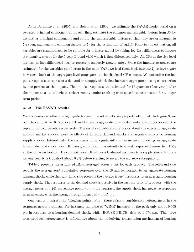
3.1.2 The FAVAR results

We first assess whether the aggregate housing market shocks are properly identified. In Figure 3, we

plot the cumulative IRFs of local HP in 41 cities to aggregate housing demand and supply shocks on the

top and bottom panels, respectively. The results corroborate our priors about the effects of aggregate

housing market shocks: positive effects of housing demand shocks and negative effects of housing

supply shocks. Interestingly, the responses differ significantly in persistence; following an aggregate

housing demand shock, local HP rises gradually and persistently to a peak response of more than 1.5%

at the four-year horizon. By contrast, local HP shows a U-shaped response to a supply shock; it drops

for one year to a trough of about 0.3% before starting to revert toward zero subsequently.

Table 3 presents the estimated IRFs, averaged across cities for each product. The left-hand side

reports the average peak cumulative responses over the 16-quarter horizon to an aggregate housing

demand shock, while the right-hand side presents the average trough responses to an aggregate housing

supply shock. The responses to the demand shock is positive in the vast majority of products, with the

average peaks at 0241 percentage points (p.p.). By contrast, the supply shock has negative responses

in most cases, with the average trough impact of −0145 p.p.Our results illustrate the following points. First, there exists a considerable heterogeneity in the

responses across products. For instance, the price of ‘WINE’ increases at the peak only about 0005

p.p in response to a housing demand shock, while ‘HOUSE PRICE’ rises by 1674 p.p. This large

cross-product heterogeneity is informative about the underlying transmission mechanism of housing

7

market shocks to local CP. Second, the wide inter-quartile bands found in many products indicate

the substantial cross-city dispersion of shock impacts. This is likely caused by differences in local

factors (e.g., Moretti 2013, Diamond 2016). To be specific, local distribution costs, such as rents paid

by the retail establishment, wages of the retail workers, transportation and warehousing, must be a

nontrivial component of the retail good and service prices and contribute to the observed cross-city

heterogeneity.11 Finally, we find the stickiness of price responses in most products, as CP respond to

housing demand shocks with some lags, consistent with Abdallah and Lastrapes (2013).

To sum, our results from the FAVAR analysis indicate that city-level CP responds in general

positively to aggregate housing demand shocks and negatively to housing supply shocks, with the

former exerting larger impacts. The size of responses varies considerably across cities and products.

As discussed in Section 4 in more detail, we use such variations to identify the channels through which

housing markets influence local CPs.

3.2 VECM analysis

3.2.1 VECM model

Although intriguing, our FAVAR model analysis focuses on the impact of aggregate housing market

shock, rather than local housing market shock which is of growing interest in the literature. In response,

here we explore how local CPs respond to local HP shocks within the framework of a VECM. The

VECM analysis is suitable for the purpose of our study on several grounds. First, it allows for possible

interactions between HP and CP with less restrictions than the traditional structural model in which

HP is typically assumed to be exogenous.12 This feature of the VECM is appealing to a study like ours

that employs MSA data where the distinction between purely endogenous and exogenous variables is

often difficult to make. Second, the VECM approach takes into account the likely interactions between

CP and HP both in the short run and in the long run. Given that housing market shocks can affect

CPs over time as we have seen from the FAVAR analysis, it is important to measure the long-run effect

of the changes in HPs on the changes in CPs. Third, the VECM approach allows causation to run both

ways between HP and CP and hence it helps us to determine the direction of causality (predictability)

between the two variables. As shown in Figure 2, higher HPs are often associated with higher CPs,

but empirically establishing the causality from HP to CP is challenging because causal relationships

11Retail prices may also reflect a pass-through of local retail rents or land prices as part of marginal costs (along

with labor costs). However, SV claim that the relationship between retail prices and house prices was driven not by

pass-through of local land prices or rents.12Consisting of a system of equations with lagged endogenous variables, the VECM is akin to vector autoregression

(VAR) model except that it includes an error correction term to capture deviation from the long-run relationship between

endogenous variables.

8

can run from both sides over time. The VECM analysis permits us to make formal inference about

the leading/causal relationship while controlling for other relevant factors.13

With that said, implicit in our VECM analysis is the assumption that local HP changes are

exogenous without further identifying the shocks that drive the price changes, following much of the

literature. To rephrase, we use HP changes as housing market shocks without identifying its origin,

although they can be driven by either housing supply or demand shocks. Since HP per se may be

the transmission mechanism of housing demand or supply shocks rather than a source of fundamental

shocks, an ideal approach should be to considering how CP and HP jointly respond to appropriately

identified, exogenous shocks.14 Nevertheless, in the dearth of such identified shocks of local housing

markets, the exogenous HP changes can be arguably viewed as an indicator of the changes in local

housing demand, not just because our FAVAR analysis shows the dominance of aggregate housing

demand shock over supply shock, but because housing demand adjusts more quickly in the short run.

We estimate the following bivariate VECM in which HP and CP are simultaneously determined

as well as determining,∙∆∆

¸=

∙

¸+

∙

¸−1 +

X=1

∙11 1221 22

¸ ∙∆−∆−

¸+

X=0

∆− +∙

¸

(3)

where and denote fixed effects and −1 = (−1−−1) is the error correction term cap-

turing the deviation from the long-run equilibrium relationship between HP and CP. The cointegrating

vector (1−) yields a consistent estimate of the long-run relationship between the two variables. Ifthere were a deviation from the long-run relationship in the previous period (as captured by the error

correction term, −1), then either HP or CP should adjust to correct for the deviation in the current

period. The parameter (or ) captures the speed at which CP (or HP) adjusts to the long-run

equilibrium per period after a shock. If the parameter estimate of (or ) is significant, then CP

(or HP) in the current period moves to correct for the deviation. Unlike the conventional univariate

error correction model, the VECM allows the endogeneity as well as the asymmetry of the convergence

13Despite these attractive features, the VECM was not much popularly used in the study of housing market mainly

due to the lack of adequate HP data. Because most HPs are in index form, it is challenging for researchers to set up

the long-run cointegration relationship formulated in the error-correction terms. In the CPI data, for instance, both HP

and CP have the same values of 100 in the base year and the corresponding error correction term will be zero for the

cointegrating vector (1,-1). For an exception, see Gallin (2008) who studied the long-run relationship between HPs and

rents using a VECM.14 In studying the impact of HP changes on retail prices, SV adopted exclusion restrictions by using local housing

supply constraints constructed by Gyourko et al. (2008) and Saiz (2010) as instruments for local HP movements. This

IV approach, however, suffers from a couple of thorny issues. First, the popular measures of MSA-level housing supply

constraints are usually static variables (fixed over time) and hence cannot capture properly the time-varying behavior of

the relationship between HP and CP. Second, housing supply constraints could be a valid but not necessarily exogenous

instrument for HP growth (Davidoff 2013, Guren et al. 2020).

9

speed, i.e., 6= , which is useful for determining the direction of causality between HP and CP.

City fixed effects are included in both the cointegrating equation and the VECM to control for many

other factors than wage and labor market conditions that influence CPs at the city level. The lagged

terms of HP and CP contain information on short-run dynamics, such as the cyclicality of HP. We

also augment the current and lagged changes in city-level wage and unemployment rate as control

variables ( = [ ]) in eq.(3). By so doing, we can account for changes in the local economic

fundamentals, cyclicality in the local labor market, as well as labor mobility across cities.15

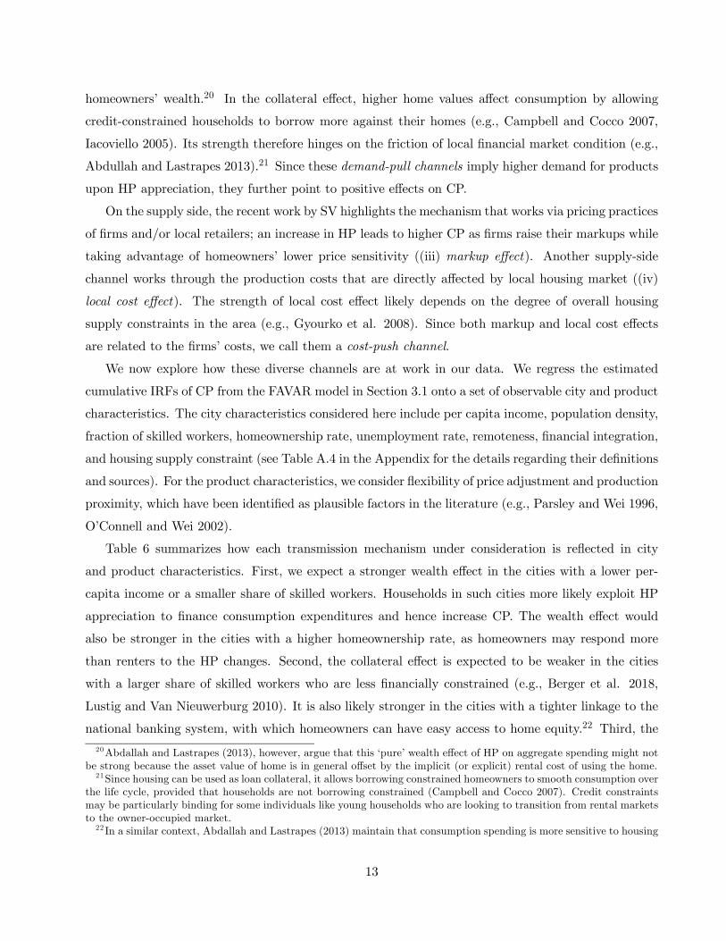
Since the VECM approach requires establishing a cointegrating relationship between variables,

we first implement a popular unit-root test, the DF-GLS test under the null hypothesis of unit-root

nonstationarity, to the city-level price series to check the prerequisite of a formal cointegration test.

As reported in Table 4, the DF-GLS test fails to reject the unit-root null for all the HP series under

study and in the vast majority of CP series, indicating strong evidence of unit-root nonstationarity

for the price series. In turn, we apply the Hausman-type cointegration test developed by Choi et al.

(2008) to the 1,763 HP-CP combinations in order to examine whether city-level HPs have a long-run

cointegration relationship with CPs. As reported in the last column of Table 4, there is strong evidence

of cointegration between HP and CP as we fail to reject the null hypothesis of cointegration in most

cases at the five percent significance level. The low rejection rate of the null hypothesis of cointegration

indicates a long-run cointegration relationship between HP and CP and hence validates our use of the

VECM approach.

3.2.2 The VECM results

The results of the city-level VECM analysis are presented in Table 5. First of all, we find compelling

evidence that local CPs are influenced by local HPs, but not vice versa. As reported in the left panel

of Table 5 (columns 1-2), is significant and positive in all products but one, while is mostly

negative and insignificant. To interpret, the deviation from the long-run equilibrium between HP and

CP is corrected primarily by the adjustment of CP, not by HP. The cross-product average of is

around 0.194, indicating that on average almost 20 percent of the gap between HP and CP is reduced

each quarter by the adjustment of CP. Not surprisingly, the adjustment speed () varies widely across

products, ranging from 0.012 (‘AUTO MAINTENANCE’) to 0.548 (‘LETTUCE’). Interestingly, the

adjustment speed of CPs appears to be faster in perishable products.

15Local wages and labor market conditions help mitigate the reverse causation from CP to HP. Van Nieuwerburgh and

Weill (2010) claim that the dispersion in MSA-level wages, reflective of local labor productivity, has been large enough

to account for the spatial distribution in HPs. Beraja et al. (2019) also emphasize the importance of local factors such as

local labor market condition in the distribution of prices. Analyzing retail prices across many U.S. metropolitan areas,

however, Coibion et al. (2015) find that changes in retail prices respond little to local unemployment rates.

10

The VECM in eq.(3) also permits us to implement the Granger (non-)causality test by looking at

whether or not changes in HP can help predict changes in CP. This is equivalent to testing the null

hypothesis that HP does not Granger cause CP (0 : 6⇒ ) with a standard F-test,

0 : = 21 = 0 for = 1

Likewise, the null hypothesis that does not Granger cause (0 : 6⇒ ) can be formulated

as 0 : = 12 = 0 for = 1 . Beware that rejecting the null hypothesis of noncausality of

HP to CP (0 : 6⇒ ) simply implies that changes in HP is helpful in predicting (forecasting)

change in CPs without providing any further assessment on the strength of the improvement in the

forecast. Columns 3 and 4 in Table 5 report the rejection rates of the nominal ten-percent Granger

causality test for each product. The rejection rate of 0 : 6⇒ is in general quite high in most

products under study, while that of 0 : 6⇒ is relatively low. This result suggests a one-way

Granger causality (or predictability) running from HP to CP, but not the other way around.16

Nevertheless, the inference from the bivariate VECM, which examines each HP-CP pair in each

city separately, could be fragile if the relationship was driven by unobservable common factors. This

concern is legitimate in our case where local prices of a product are likely to be correlated across cities,

possibly through common national factors like national supply chains.17 As a further robustness check,

we apply the panel VECM (PVECM) across all the 41 cities for each product. Following Holly et al.

(2010), we utilize the Common Correlated Effects (CCE) estimator in the PVECM to deal with the

cross-sectional dependence (CSD) and the unobserved common factor issues, after controlling for local

wages and labor market conditions as before. The CCE estimators are based on a multifactor error

structure, which controls for unobserved common factors as well as spatial effects of price changes.18

The right panel of Table 5 reports the PVECM results, which largely corroborate the results

obtained from the city-level bivariate VECM. Albeit not as strong as before, we still find evidence of

the one-way causality running from HP to CP, i.e., CPs are responsive to HP, but not the other way

around.19 The coefficient of is statistically significant in almost half of the products under study,

16This outcome is in line with the finding by SV on the causal response of local retail prices to changes in local HPs,

based on different shock identifications.17HPs are also likely correlated across MSAs, not just through common macro factors, such as the interest rate, that

affect HPs in all MSAs, but also through spatial effects, i.e., HP changes in a MSA affect those in other MSAs. In

this context, CPs in a MSA can be affected by HP changes in other MSAs. In the presence of the multifactor (both

common factor and spatial effect), the usual OLSE is biased as the error terms are correlated to the common factor of

the explanatory variable by nature.18The CCE estimators are constructed using regressions augmented with cross-sectional averages of all dependent and

independent variables. As shown by Pesaran (2006), the cross-sectional averages of dependent and independent variables

effectively control for the unobserved common factors.19The weaker evidence of causality running from HP to CP in the PVECM must have arisen from the fact that the

influences of common national factors are effectively removed by using the CCE estimates. This is particularly relevant

for some products that are typically produced nationally (e.g., ‘SHORTENING’).

11

while the coefficient of is significant in no products. Interestingly, the long-run causal relationship

running from HP to CP is found more frequently in food and rent related products that are more

influenced by local factors. Again, a wide variation exists in the speed of adjustment () across

products. CPs of some products adjust to HP much faster than those in other products. In general, the

adjustment speed appears to be faster for non-durable products which are typically produced locally

in a more competitive environment, compared to manufacturing goods that are produced nationally.

The fastest adjustment speed was found in ‘GROUND BEEF’ (almost 39 percent per quarter), while

the adjustment speed is very slow for ‘MEN’S SHIRT’ (less than 1 percent per quarter). As presented

in the last column of Table 5, the long-run effect (LRE) of a unit-shock of HP onto CP also varies

widely from 0.024 (MAN’S SHIRT) to 0.994 (GASOLINE), i.e., the local gasoline price is a lot more

responsive cumulatively to a change in local HP. The average LRE across products is around 0.46, i.e.,

a 10% increase in HPs is associated with around 4.6% increase in CPs. This estimate is higher than the

cross-sectional elasticity of CP to HP (0.15-0.20) reported by SV. As discussed in more detail in Section

4.3, the difference between the two studies stems from a variety of sources, including the differences

in data coverage, identification of shocks, time horizons of shock impacts, and methodologies.

4 Transmission channels of housing markets to CPs

Our analysis so far suggests that the impact of housing market shocks on local CP is nontrivial and

persists over time. More importantly, substantial heterogeneity was found in the response across cities

and across products. This heterogeneity contains useful information about underlying transmission

mechanism. Previous literature has featured a range of transmission channels, some of which can be

simultaneously at work to different degrees, resulting in the observed heterogeneous responses. In this

section, we attempt to disentangle those different channels based on the cross-city and cross-product

heterogeneities found in our data. To that end, we conduct a second-stage regression analysis to gauge

the importance of competing transmission mechanisms by relating the estimated impacts to a variety

of city- and product-specific characteristics.

4.1 Transmission mechanisms of housing market shocks to CPs

The channels through which HP changes affect consumption has garnered enormous and growing

attention from both policymakers and academic researchers. The existing literature offers two major

channels through which changes in HP affect consumption spending: the (i) wealth effect and (ii)

collateral effect. According to the wealth effect, higher HP increases consumption spending by raising

12

homeowners’ wealth.20 In the collateral effect, higher home values affect consumption by allowing

credit-constrained households to borrow more against their homes (e.g., Campbell and Cocco 2007,

Iacoviello 2005). Its strength therefore hinges on the friction of local financial market condition (e.g.,

Abdullah and Lastrapes 2013).21 Since these demand-pull channels imply higher demand for products

upon HP appreciation, they further point to positive effects on CP.

On the supply side, the recent work by SV highlights the mechanism that works via pricing practices

of firms and/or local retailers; an increase in HP leads to higher CP as firms raise their markups while

taking advantage of homeowners’ lower price sensitivity ((iii) markup effect). Another supply-side

channel works through the production costs that are directly affected by local housing market ((iv)

local cost effect). The strength of local cost effect likely depends on the degree of overall housing

supply constraints in the area (e.g., Gyourko et al. 2008). Since both markup and local cost effects

are related to the firms’ costs, we call them a cost-push channel.

We now explore how these diverse channels are at work in our data. We regress the estimated

cumulative IRFs of CP from the FAVAR model in Section 3.1 onto a set of observable city and product

characteristics. The city characteristics considered here include per capita income, population density,

fraction of skilled workers, homeownership rate, unemployment rate, remoteness, financial integration,

and housing supply constraint (see Table A.4 in the Appendix for the details regarding their definitions

and sources). For the product characteristics, we consider flexibility of price adjustment and production

proximity, which have been identified as plausible factors in the literature (e.g., Parsley and Wei 1996,

O’Connell and Wei 2002).

Table 6 summarizes how each transmission mechanism under consideration is reflected in city

and product characteristics. First, we expect a stronger wealth effect in the cities with a lower per-

capita income or a smaller share of skilled workers. Households in such cities more likely exploit HP

appreciation to finance consumption expenditures and hence increase CP. The wealth effect would

also be stronger in the cities with a higher homeownership rate, as homeowners may respond more

than renters to the HP changes. Second, the collateral effect is expected to be weaker in the cities

with a larger share of skilled workers who are less financially constrained (e.g., Berger et al. 2018,

Lustig and Van Nieuwerburg 2010). It is also likely stronger in the cities with a tighter linkage to the

national banking system, with which homeowners can have easy access to home equity.22 Third, the

20Abdallah and Lastrapes (2013), however, argue that this ‘pure’ wealth effect of HP on aggregate spending might not

be strong because the asset value of home is in general offset by the implicit (or explicit) rental cost of using the home.21Since housing can be used as loan collateral, it allows borrowing constrained homeowners to smooth consumption over

the life cycle, provided that households are not borrowing constrained (Campbell and Cocco 2007). Credit constraints

may be particularly binding for some individuals like young households who are looking to transition from rental markets

to the owner-occupied market.22 In a similar context, Abdallah and Lastrapes (2013) maintain that consumption spending is more sensitive to housing

13

markup effect is expected to be inversely related to city population density, where firms would have

lower pricing power as markets are more competitive (e.g., Handbury and Weinstein 2015). Instead, it

is likely stronger in the cities that are geographically and economically isolated, which makes it easier

for firms to exercise their pricing power. It would be also negatively related to local unemployment,

as markup rates are well-known to be cyclical (see for example, Nekarda and Ramey 2013). Finally,

we expect stronger local cost effects in the cities where housing supply constraints are more stringent,

thus HP changes results in larger impacts on local costs such as rents.

Of the two product characteristics we consider, the first one is the price adjustment flexibility.

It can be viewed as a proxy for the degree of market competition, as prices are likely adjusted more

flexibly in more competitive markets. Since markup rates are expected to be lower in more competitive

markets, the price flexibility is also related (negatively) to the markup effect. In our analysis, we divide

the products into three groups based on the degree of price flexibility: (i) most flexibly priced; (ii)

medium flexibly priced; and (iii) least flexibly priced groups.23

The second product characteristics is the production proximity to marketplace, which reflects

product-level market frictions as well as markup rates. For example, as many of the nationally pro-

duced and distributed products are branded, firms producing those products can exercise more pricing

power. In the case of locally-produced products, the price setting power of producers would be limited

because consumers would have lower allegiance to specific products. Hence, we expect the markup

effects would be negatively related to the production proximity. In contrast, the local cost channel is

expected to be stronger for locally-produced products. Since the latter, such as milk, are difficult to

transport, they are more influenced by local production costs like rent. Following O’Connell and Wei

(2002), products are also sorted into three groups based on the production proximity: (i) generally

not locally-produced products (Category A); (ii) maybe locally-produced products (Category B); and

(iii) always locally-produced products (Category C).

4.2 Regression analysis for identifying transmission mechanisms

We conduct the following cross-section regression analysis in which the cumulative IRF estimates from

the FAVAR models are regressed on the set of the aforementioned city and product characteristics

variables,

= +

2X=1

+0 + for = 1 43 = 1 41 = 0 4 (4)

demand shocks in states with better-developed financial institutions.23We obtain the price flexibility data for our products by utilizing the extensive data set constructed by Nakamura

and Steinsson (2008). See Table A.1 for details.

14

where represents the h-year median cumulative effect of housing market shocks on the price of

the product in city . denotes a product dummy variable for three product groups based on

either the price flexibility (for the housing demand shock) or the production proximity (for the housing

supply shock). is the set of city characteristics discussed earlier. is the error term that can

be cross-sectionally correlated and possibly heteroskedastic. Because standard heteroskedastic robust

standard errors may overstate the true standard errors in the presence of a high degree of clustering

among the city and product combinations, we use robust clustered standard errors.24 We conduct two

sets of regression analyses with the IRFs to housing demand and supply shocks separately.

The regression results are reported in Table 7. We first note a difference in the significance of

explanatory variables between the two different housing market shocks. For housing demand shocks,

city characteristics such as the share of skilled workers and remoteness turn out to be consistently

significant in explaining its pass-through. The result of the skilled worker share is consistent with

the finding by Moretti (2013) on a systematic positive relationship between HP and the number of

college graduates in a city. These, however, do not much line up with the demand-pull channel. The

insignificance of per capita income and the unexpected negative sign of the share of homeownership

run counter to the wealth effect argument, while the insignificance of financial integration further

weakens the relevance of the collateral effect.25 Nonetheless, we find that housing demand shocks

have significant impacts on CPs in the products whose prices are adjusted more frequently, in line

with our prior that firms would respond quickly to the increased product demand from the wealth or

collateral effects.26 Collectively, our results partly support the demand-pull channel as it is at work

in the transmission of housing demand shock across products, but not necessarily across space.

Turning to the results for supply shocks, we no longer see the significance of the skilled worker

share. Instead, housing supply constraint and homeownership rate are consistently significant for

explaining the cross-city differences in their pass-through. Hence, they provide evidence supporting

the local cost and markup effects, respectively.27 For the product characteristics, the result implies

that the supply shocks spill over significantly more to the locally-produced products, compared to the

nationally-produced ones. This outcome further supports the local cost effect, but not the markup

effect. Taken together, the transmission mechanism of housing supply shock is better aligned with the

24Since the impacts of housing market shocks are more likely correlated across cities for a given product, rather than

across products for a given location, standard errors are clustered by observations by cities rather than by products.25This result differs from Abdallah and Lastrapes (2013) who find supportive evidence of the collateral effect using the

state-level consumption expenditure data.26This outcome, however, is at odds with the recent finding by Beraja et al. (2019) that nominal wage rigidity plays a

more important role than price stickiness in the transmission of local economic shocks during the Great Recession. The

authors also argue that prices respond very quickly to changes in local economic conditions, but not to housing market

shocks, which is quite different from what is found in the current study.27The homeownership rate is generally higher in smaller cities where firms’ market power is stronger.

15

cost-push channel via local cost effect. The markup effect is at work at the city level, but not at the

product level.

In sum, our results suggest that the nature of housing market shocks matters for the transmission

mechanisms. Whereas housing demand shock is mainly transmitted to CP through the demand-pull

channel, housing supply shock is transmitted primarily through the cost-push channel. Moreover, it

seems improbable that any one transmission mechanism in isolation would be sufficient to explain the

impact of housing markets on local CPs.

4.3 Further discussions on the empirical findings

As noted in the introduction, our paper is closely related to the recent work by SV. Despite the similar

conclusions reached about the impact of HP and CP, the two studies differ, in particular with respect

to the details of the relevant transmission mechanism. To begin, while SV highlight the changes in

markups as the primary channel, we find that the markup effect is at work only in the transmission

of housing supply shocks. Moreover, SV did not find the relevance of local retail rents or land prices.

Furthermore, whereas SV find that HP changes affect the retail price mainly through homeowners, we

show that homeownership mitigates the transmission of a housing demand shock, but intensifies the

effects of a housing supply shock.

In addition, the results from two studies also differ with regard to the role of price flexibility. We

find that housing demand shocks transmit faster to the products whose prices adjust more frequently.

By contrast, SV contend that firms’ pricing-to-market practice is the primary channel, as firms charge

higher prices in locations with higher HP. Since markup rates would be smaller for the products with

frequently-adjusted prices, one might infer that our findings do not accord with theirs regarding the

role of price flexibility.

To ensure that our results on the role of price flexibility are not an artifact of specific empirical

methods, we further delve into this issue using the results obtained from the VECM analysis. Specifi-

cally, we examine the relationship between the degree of price flexibility and the estimated adjustment

speed of CP ( in eq.(3)) across products. Intuitively, how fast prices can adjust to a shock might

hinge on how quickly CP can correct for the deviation from the long-run equilibrium. More impor-

tantly, one would expect a faster adjustment of CP to the deviation in the products with more frequent

price adjustment. As illustrated in the top panel of Figure 4, we indeed find a positive association

between the adjustment speed () and the degree of price flexibility across 41 products. We also

look at the relationship between the price flexibility and the long-run effect estimates from the Panel

VECM, reported in the last column of Table 5. As shown in the bottom panel of Figure 4, we again

16

find a positive association. These results reinforce our previous findings from the FAVAR model that

price flexibility plays an important role in the transmission mechanism.

That being said, the difference between the two studies could arise from a variety of sources,

including data coverage, econometric methodology, and time horizon of shock response, as summarized

in more detail in Table 1. For instance, while we employ the data set covering a wide range of products

including food, manufacturing goods, and services, SV focus on tradable goods only that are generally

sold in grocery stores or drugstores. Those goods are typically produced nationally, and hence, are

not much susceptible to local shocks. This may explain why the significant effect of local cost is found

in our study, but in SV. We also note that the two studies focus on different time horizons. While

SV focus on the cross-sectional elasticity, our main interest is in the cumulative long-run effects. The

latter can be quite different from the former, as shocks can take time to propagate and their impacts

may exhibit some nonlinear patterns over time.

Differences in the sample periods also turn out to be consequential. To investigate this issue, we

estimate the elasticity of local retail prices to HP movements in the spirit of SV (eqs.(1)-(2) in p.1409)

using our data. For this exercise, we focus on the 11 processed food-related products in our data,

to retain similarity with the ones considered by SV. Also, we use the housing supply elasticity from

Guren et al. (2020) as an instrument, instead of the Saiz’s (2010) measure employed by SV. We find

that the average elasticity of local retail prices to HP is around 10.7 percent over the period 2001-2011,

which is much smaller than the cumulative long-run effect found in Section 3.2, but close to the range

of 15-20 percent reported by SV.

We further look at the stability of our findings over time using a rolling window estimation. Figure

5 plots the mean and interquartile ranges of the long-run effects among 43 products, estimated from

the Panel VECM using a 10-year rolling window. As displayed in figure 5, the mean has been stable

around 0.4 until the period of 1998-2007 when it started rising to around 0.6 and then declined steadily

toward zero.28 A similar pattern is noted in the interquartile ranges of the estimates, suggesting that

the time-varying behavior is significant across all products under study. Interestingly, the time-varying

estimates appear to align with the housing boom-bust cycle in the 2000s (e.g., Gelain et al. 2018).

Specifically, the pass-through was stronger during housing boom when HP rose fast, then weakened

during housing bust period. This finding lends credence to the claim by Guren et al. (2020) that it

is challenging to discern between a cyclical pattern and the causal relationship between HP and CP

based on a single cross-section regression. All in all, we view that our paper compliments and extends

28The decline in the responsiveness of CPs to HP in recent years might have come from the increased pricing power of

firms in the U.S. due to reduced competition in many industries. In a more concentrated market, firms can time their

pricing to maximize profits and thus absorb housing market shocks. Relatedly, Heise et al. (2020) attribute the decline

in the pass-through of wages to goods prices to rising import competition and increased market concentration.

17

the work by SV.

5 Concluding remarks

Housing markets have long been recognized to be important for the overall economy, in particular

due to the potential influences of housing values on consumption spending. Yet, few studies have

focused on the impact of housing markets on local CP. Given that housing typically takes up a major

proportion of household net worth for most homeowners, a change in HP could have a significant effect

on CP possibly through consumption spending and shopping behavior (e.g., Aguiar and Hurst 2007,

Kaplan and Menzio 2013). HP may also affect CP via the cost of local services or rents especially in

cities where housing/land is more expensive.

In this paper, we investigated whether, to what extent, and through which channels housing

markets affect local CP, using retail price data collected for the selected U.S. cities over the past 25

years. Within the framework of FAVAR and VECM, our empirical analysis revealed that most local

CP were highly responsive to the changes in local HP, but not the other way around. Controlling

for city-level income and local labor market conditions, we found that on average a 10% rise in HP

leads to around 4.6% increases in CP over time. The leading/causal effects of housing markets on

local CP, however, differ markedly depending on the nature of shocks. While housing demand shocks

have persistently positive effects on CP, supply shocks exhibit transitory negative impacts. Significant

heterogeneity was also found in the size of effects across products as well as locations. We exploited

the heterogeneous responses to explore the potential underlying channels of pass-through by linking

the estimated responses of CP to a set of observable factors identified in the literature as reflecting

underlying transmission mechanisms. We found much stronger responses of CP to the housing demand

shocks in the cities that have higher shares of skilled workers and in the products whose prices are

adjusted more frequently. The responses to the housing supply shocks turned out to be stronger in

the cities with tighter housing supply regulations and for the locally-produced products. Collectively,

our results support the demand-pull channel for the pass-through of the hosing demand shock, and

the cost-push channel for the hosing supply shock.

Our findings had further implications on the measure of cost-of-living and consumer welfare. Hous-

ing market fluctuations have an impact on CPI directly by affecting the shelter index (or user cost)

and indirectly through the spillover effects on local CP over time. Together, HP may have substantial

influences upon the overall cost-of-living and consumer welfare. Understanding the link between HP

and CP also offers useful insights into the geographic dispersions of cost-of-living and thus geographic

economic inequality (e.g., Hsieh and Moretti 2015). Our result that homeownership mitigates the

18

transmission of a housing demand shock while intensifies the effects of a housing supply shock, further

notes the source of inequality across cities.

19

20

References [1] Aastveit, Knut Are, Bruno Albuquerque and André Anundsen, 2020. “Changing Supply

Elasticities and Regional Housing Booms.” Staff Working Paper No. 844, Bank of England.

[2] Abdallah, Chadi S. and William D. Lastrapes, 2013. “Evidence on the Relationshipbetween Housing and Consumption in the United States: A State-Level Analysis.”Journal of Money, Credit and Banking, 45(4), 559—589. https://doi.org/10.1111/jmcb.12016

[3] Aguiar, Mark, and Erik Hurst, 2007. “Life-Cycle Prices and Production.” AmericanEconomic Review, 97(5), 1533—1559. https://doi.org/10.1257/aer.97.5.1533

[4] Bajari, Patrick, C. Lanier Benkard and John Krainer, 2005. “House Prices and ConsumerWelfare.” Journal of Urban Economics, 58, 474—487. https://doi.org/10.1016/j.jue.2005.08.008

[5] Beraja, Martin, Erik Hurst and Juan Ospina, 2019. “The Aggregate Implications of RegionalBusiness Cycles.” Econometrica, 87(6), 1789—1833. https://doi.org/10.3982/ECTA14243

[6] Berger, David, Veronica Guerrieri, Guido Lorenzoni and Joseph Vavra, 2018. “House Pricesand Consumer Spending.” Review of Economic Studies, 85(3), 1502—1542.https://doi.org/10.1093/restud/rdx060

[7] Bernanke, Ben S., Jean Boivin and Piotr Eliasz, 2005. “Measuring the Effects of MonetaryPolicy: A Factor-augmented Vector Autoregressive (FAVAR) Approach.” Quarterly Journal ofEconomics, 120(1), 387—422. https://doi.org/10.1162/0033553053327452

[8] Boivin, Jean, Marc Giannoni and Ilian Mihov, 2009. “Sticky Prices and Monetary Policy:Evidence from Disaggregated US Data.” American Economic Review, 99(1), 350—384.https://doi.org/10.1257/aer.99.1.350

[9] Bhutta, Neil, and Benjamin J. Keys, 2016. “Interest Rates and Equity Extraction Duringthe Housing Boom.” American Economic Review, 106(7), 1742—1774.https://doi.org/10.1257/aer.20140040

[10] Campbell, John Y., and João F. Cocco, 2007. “How Do House Prices Affect Consumption?Evidence from Micro Data.” Journal of Monetary Economics, 54(3), 591—621.https://doi.org/10.1016/j.jmoneco.2005.10.016

[11] Cecchetti, Stephen, 2007. “Housing in Inflation Measurement.” https://voxeu.org/articles/housing-inflation-measurement

[12] Choi, C.Y., and J. Andrew Hansz, 2020. “From Banking Integration to Housing MarketIntegration - Evidence from U.S. Metropolitan Housing Prices.” mimeo, University of Texas atArlington.

[13] Choi, C.Y., Ling Hu, and Masao Ogaki, 2008. “Robust estimation for Structural SpuriousRegressions and a Hausman-type Cointegration Test.” Journal of Econometrics, 142, 327—351. https://doi.org/10.1016/j.jeconom.2007.06.003

[14] Coibion, Olivier, Yuriy Gorodnichenko and Gee Hee Hong, 2015. “The Cyclicality of Sales,Regular and Effective Prices: Business Cycle and Policy Implications.” American EconomicReview, 105(3), 993—1029. https://doi.org/10.1257/aer.20121546

[15] Davidoff, Thomas, 2013. “Supply Elasticity and the Housing Cycle of the 2000s.” Real EstateEconomics, 41(4), 793—813. https://doi.org/10.1111/1540-6229.12019

[16] DellaVigna, Stefano and Matthew Gentzkow, 2019. “Uniform Pricing in US Retail Chains.”Quarterly Journal of Economics, 134(4), 2011—2084. https://doi.org/10.1093/qje/qjz019

[17] Diamond, Rebecca, 2016. “The Determinants and Welfare Implications of US Workers’Diverging Location Choices by Skill: 1980—2000.” American Economic Review, 106(3),479—524. https://doi.org/10.1257/aer.20131706

21

[18] Gallin, Joshua, 2008. “The Long-Run Relationship Between House Prices and Rents.” RealEstate Economics, 36(4), 635—658. https://doi.org/10.1111/j.1540-6229.2008.00225.x

[19] Gelain, Paolo, Kevin J. Lansing, and Gisle J. Natvik, 2018. “Explaining the Boom-Bust Cyclein the U.S. Housing Market: A Reverse-Engineering Approach.” Journal of Money, Credit andBanking, 50(8), 1751—1783. https://doi.org/10.1111/jmcb.12504

[20] Ghent, Andra C., and Michael T. Owyang, 2010. “Is Housing the Business Cycle? Evidencefrom US Cities.” Journal of Urban Economics, 67, 336—351.https://doi.org/10.1016/j.jue.2009.11.001

[21] Green, Richard K., Stephen Malpezzi, and Stephen K. Mayo, 2005. “Metropolitan-Specific Es- timates of the Price Elasticity of Supply of Housing, and Their Sources.” American EconomicReview, 95(2), 334—339. https://doi.org/10.1257/000282805774670077

[22] Guren, Adam M., Alisdair McKay, Emi Nakamura, and Jon Steinsson, 2020. “Housing WealthEffects: The Long View.” Review of Economic Studies, forthcoming.https://doi.org/10.1093/restud/rdaa018

[23] Gyourko, Joseph, Albert Saiz, and Anita Summers, 2008. “A New Measure of the Local Regula- tory Environment for Housing Markets: The Wharton Residential Land Use RegulatoryIndex.” Urban Studies, 45(3), 693—729. https://doi.org/10.1177/0042098007087341

[24] Handbury, Jessie, and David E. Weinstein, 2012. “Goods Prices and Availability in Cities.”Review of Economic Studies, 82, 258—296. https://doi.org/10.1093/restud/rdu033

[25] Heise, Sebastian, Fatih Karahan, and Aysegül Sahin, 2020. “The Missing Inflation Puzzle:The Role of the Wage-Price Pass-Through.” NBER Working Papers No. 27663, NationalBureau of Economic Research. https://doi.org/10.3386/w27663

[26] Holly, Sean, M. Hashem Pesaran, and Takashi Yamagata, 2010. “A Spatio-temporal Modelof House Prices in the USA.” Journal of Econometrics, 158, 160—173.https://doi.org/10.1016/j.jeconom.2010.03.040

[27] Hsieh, Chang-Tai, and Enrico Moretti, 2015. “Why Do Cities Matter? Local Growth andAggregate Growth.” NBER Working Papers No. 21154, National Bureau of EconomicResearch.

[28] Iacoviello, Matteo, 2005. “House Prices, Borrowing Constraints, and Monetary Policy in theBusiness Cycle.” American Economic Review, 95(3), 739—764.https://doi.org/10.1257/0002828054201477

[29] Iacoviello, Matteo, and Stefano Neri, 2010. “Housing Market Spillovers: Evidence from anEstimated DSGE Model.” American Economic Journal: Macroeconomics, 2(2), 125—64.https://doi.org/10.1257/mac.2.2.125

[30] Jarocinski, Marek, and Frank Smets, 2008. “House Prices and the Stance of MonetaryPolicy.” ECB Working Paper Series No. 891, The European Central Bank.

[31] Jayaratne, Jith, and Donald P. Morgan, 2000. “Capital Market Frictions and DepositConstraints at Banks.” Journal of Money, Credit and Banking, 32(1), 74—92.https://doi.org/10.2307/2601093

[32] Kaplan, Greg, and Guido Menzio, 2016. “Shopping Externalities and Self-FulfillingUnemployment Fluctuations.” Journal of Political Economics, 124(3), 771—825.https://doi.org/10.1086/685909

[33] Kuhn, Moritz, Moritz Schularick, and Ulrike I. Steins, 2020. “Income and Wealth Inequality inAmerica, 1949-2016.” Journal of Political Economy, forthcoming.https://doi.org/10.1086/708815

[34] Lustig, Hanno, and Stijn Van Nieuwerburgh, 2010. “How Much Does Household CollateralConstrain Regional Risk Sharing?” Review of Economic Dynamics, 13(2), 265—294.

22

https://doi.org/10.1016/j.red.2009.09.005

[35] Mian, Atif, and Amir Sufi, 2011. “House Prices, Home Equity-Based Borrowing, and theU.S. Household Leverage Crisis.” American Economic Review, 101(5), 2132—2156.https://doi.org/10.1257/aer.101.5.2132

[36] Mian, Atif, and Amir Sufi, 2014. “What Explains the 2007-2009 Drop in Employment?”Econometrica, 82(6), 2197—2223. https://doi.org/10.3982/ECTA10451

[37] Mian, Atif, Kamalesh Rao, and Amir Sufi, 2013. “Household Balance Sheets, Consumption,and the Economic Slump.” Quarterly Journal of Economics, 128(4), 1687—1726.https://doi.org/10.1093/qje/qjt020

[38] Moretti, Enrico, 2013. “Real Wage Inequality.” American Economic Journal: Applied Economics,5(1), 65—103. https://doi.org/10.1257/app.5.1.65

[39] Nakamura, Emi, and Jon Steinsson, 2008, “Five Facts about Prices: A Reevaluation ofMenu Cost Models.” Quarterly Journal of Economics 123, 1415—64.https://doi.org/10.1162/qjec.2008.123.4.1415

[40] Nekarda, Christopher J., and Valerie A. Ramey, 2013. “The Cyclical Behavior of the Price-Cost Markup.” NBER Working Papers No. 19099, National Bureau of Economic Research.https://doi.org/10.3386/w19099

[41] O’Connell, Paul G.J., and Shang-Jin Wei, 2002. ““The Bigger They Are, The Harder TheyFall”: Retail Price Differences across U.S. Cities.” Journal of International Economics 56(1),21—53. https://doi.org/10.1016/S0022-1996(01)00111-8

[42] Parsley, David C., and Shang-Jin Wei, 1996. “Convergence to the Law of One PriceWithout Trade Barriers or Currency Fluctuations.” Quarterly Journal of Economics 111,1211—1236. https://doi.org/10.2307/2946713

[43] Pesaran, M. Hashem, 2006. “Estimation and Inference in Large Heterogeneous Panels with aMultifactor Error Structure.” Econometrica, 74(4), 967—1012.https://doi.org/10.1111/j.1468-0262.2006.00692.x

[44] Saiz, Albert, 2010. “The Geographic Determinants of Housing Supply.” Quarterly EconomicJournal, 125(3), 1253—1296. https://doi.org/10.1162/qjec.2010.125.3.1253

[45] Sheiner, Louise, 1995. “Housing Prices and the Savings of Renters.” Journal of UrbanEconomics, 38, 94—125. https://doi.org/10.1006/juec.1995.1024

[46] Sinai, Todd M., 2012. “House Price Moments in Boom-Bust Cycles.” NBER Working Papers No.18059, National Bureau of Economic Research. https://doi.org/10.3386/w18059

[47] Stroebel, Johannes, and Joseph Vavra, 2019. “House Prices, Local Demand, and RetailPrices.” Journal of Political Economics, 127(3), 1391—1436. https://doi.org/10.1086/701422

[48] Van Nieuwerburgh, Stijn, and Pierre-Olivier Weill, 2010. “Why Has House Price DispersionGone Up?” Review of Economic Studies, 77, 1567—1606. https://doi.org/10.1111/j.1467-937X.2010.00611.x

[49] Waxman, Andrew, Yuanning Liang, Shanjun Li, Panle Jia Barwickc, and Meng Zhao,2020. “Tightening belts to buy a home: Consumption responses to rising housing prices inurban China.” Journal of Urban Economics, 115, 103190.https://doi.org/10.1016/j.jue.2019.103190

[50] Wolf, Holger C., 2000. “Intranational Home Bias in Trade.” Review of Economics and Statistics,82(4), 555—563. https://doi.org/10.1162/003465300559046

[51] Yoshida, Jiro, 2015. “Stock Prices, Regional Housing Prices, and Aggregate TechnologyShocks.” mimeo, Penn State University.

Table 1: Comparison with the work by Stroebel and Vavra (2019)

The current study Stroebel and Vavra (2019)

Data coverage Quarterly survey retail price in 41 Weekly IRI scanner data for 31

cities for 43 products for food, grocery and drugstore products

manufacturing, and service over the over 2001-2011

period 1990-2015

Shock Aggregate housing shocks identified IV approach using the Saiz’s (2010)

identification in FAVAR model and HP changes in housing supply elasticity as an

the VECM instrument

Time horizon Both short-run and long-run effect of Cross-sectional elasticity of CP

HP to CP to HP

Transmission Wealth effect and collateral effect Markup effect

mechanism for housing demand shock transmission; No effect of local costs or rents

Markup effect and local cost effect

for housing supply transmission

Quantitative effect Average long-run effect of 0.45 Elasticity of 0.15-0.20

effect of HP on CP

The role of price Yes No

flexibility

Significance of Yes for the transmission of housing Yes for the cross-city difference

homeownership supply shock, but not for housing in the elasticity of HP to CP

demand shock

Econometric FAVAR, VECM, and cross-sectional Cross-sectional regression

methodologies regression

Table 2: Sign Restrictions

Variables Housing Demand Shock Housing Supply Shock

Real residential investment positive positive

House prices positive negative

5-yr rate − −GDP deflator − −Real GDP − −Real PCE − −Unobservable factors () − −

Note: This table summarizes how we impose sign restrictions to identify housing demand ad supply shocks. Therestrictions are imposed for three quarters after the impact on real residential investment and house prices only, whilesigns of other variables are left unrestricted (noted as “−” in the table).

23

Table 3: Peak responses of CPs to housing demand and supply shocks from FAVAR model

Product Demand shock Supply shock

Average [25%,75%] Average [25%,75%]

Steak 0.416 [ 0.245, 0.512] 0.030 [-0.112, 0.225]

Ground beef 0.262 [ 0.077, 0.400] -0.092 [-0.254, 0.115]

Whole chicken 0.234 [ 0.022, 0.327] -0.168 [-0.441, 0.038]

Canned tuna 0.096 [ 0.048, 0.159] -0.315 [-0.501, -0.135]

Milk 0.420 [ 0.185, 0.543] 0.093 [-0.055, 0.214]

Eggs 0.078 [ 0.005, 0.177] 0.059 [-0.006, 0.183]

Margarine 0.107 [ 0.005, 0.189] -0.155 [-0.333, -0.057]

Cheese 0.081 [-0.134, 0.149] -0.173 [-0.302, 0.037]

Potatoes 0.608 [ 0.478, 0.748] -0.043 [-0.180, 0.047]

Bananas 0.077 [-0.081, 0.120] -0.055 [-0.143, 0.065]

Lettuce 0.102 [0.050, 0.176] -0.410 [-0.632, -0.261]

Bread 0.136 [-0.043, 0.209] -0.037 [-0.258, 0.209]

Coffee -0.133 [-0.252, 0.096] 0.093 [-0.090, 0.281]

Sugar 0.011 [-0.090, 0.041] -0.268 [-0.392, -0.132]

Corn flakes 0.157 [-0.042, 0.255] -0.104 [-0.249, 0.051]

Canned peas 0.191 [-0.016, 0.302] -0.334 [-0.551, -0.053]

Canned peaches 0.182 [-0.050, 0.250] -0.294 [-0.442, -0.162]

Tissue 0.254 [ 0.033, 0.498] -0.314 [-0.557, -0.110]

Detergent 0.211 [ 0.092, 0.283] -0.332 [-0.521, -0.152]

Shortening 0.566 [ 0.259, 0.682] -0.490 [-0.655, -0.310]

Frozen corn 0.171 [-0.024, 0.322] -0.084 [-0.222, 0.126]

Soft drink 0.182 [ 0.004, 0.227] -0.249 [-0.443, -0.027]

Apartment rent 0.356 [ 0.022, 0.409] -0.008 [-0.207, 0.146]

House price 1.674 [ 1.167, 1.954] -0.363 [-0.607, -0.163]

Telephone 0.248 [-0.041, 0.322] -0.286 [-0.525, -0.134]

Auto maintenance 0.150 [ 0.070, 0.227] -0.322 [-0.399, -0.243]

Gas 0.204 [ 0.129, 0.247] -0.580 [-0.652, -0.532]

Doctor visit 0.137 [-0.009, 0.285] -0.118 [-0.328, 0.066]

Dentist visit 0.072 [-0.059, 0.068] -0.194 [-0.378, -0.004]

Hamburger -0.008 [-0.121, 0.013] -0.253 [-0.466, -0.013]

Pizza 0.575 [ 0.170, 0.911] -0.251 [-0.530, 0.022]

Fried chicken 0.225 [-0.036, 0.339] -0.269 [-0.528, -0.011]

Man’s haircut 0.213 [-0.015, 0.337] -0.222 [-0.500, 0.098]

Beauty salon 0.193 [ 0.000, 0.370] -0.171 [-0.481, 0.027]

Toothpaste 0.208 [ 0.054, 0.354] -0.028 [-0.069, 0.147]

Dry cleaning 0.164 [-0.096, 0.271] -0.197 [-0.386, 0.067]

Man’s shirt 0.139 [ 0.032, 0.201] 0.098 [-0.066, 0.258]

Appliance repair 0.252 [ 0.025, 0.386] -0.119 [-0.346, 0.025]

Newspaper 0.144 [-0.031, 0.219] -0.191 [-0.473, -0.045]

Movie 0.075 [-0.048, 0.141] -0.404 [-0.578, -0.171]

Bowling 0.174 [-0.032, 0.268] -0.095 [-0.284, 0.036]

Tennis balls 0.183 [-0.030, 0.402] -0.095 [-0.252, 0.103]

Beer 0.634 [ 0.469, 0.815] -0.434 [-0.525, -0.330]

Wine 0.005 [-0.109, 0.057] -0.358 [-0.550, -0.205]

Note: Entries represent the average peak (for demand shock) and trough (for supply shock) responses of CPs to housing

market shock and the corresponding intercity quartile (25- and 75-percentiles) across cities. Impulse responses are normalizedresponses to each shock that increases private residential fixed investment by 1% at the impact.

24

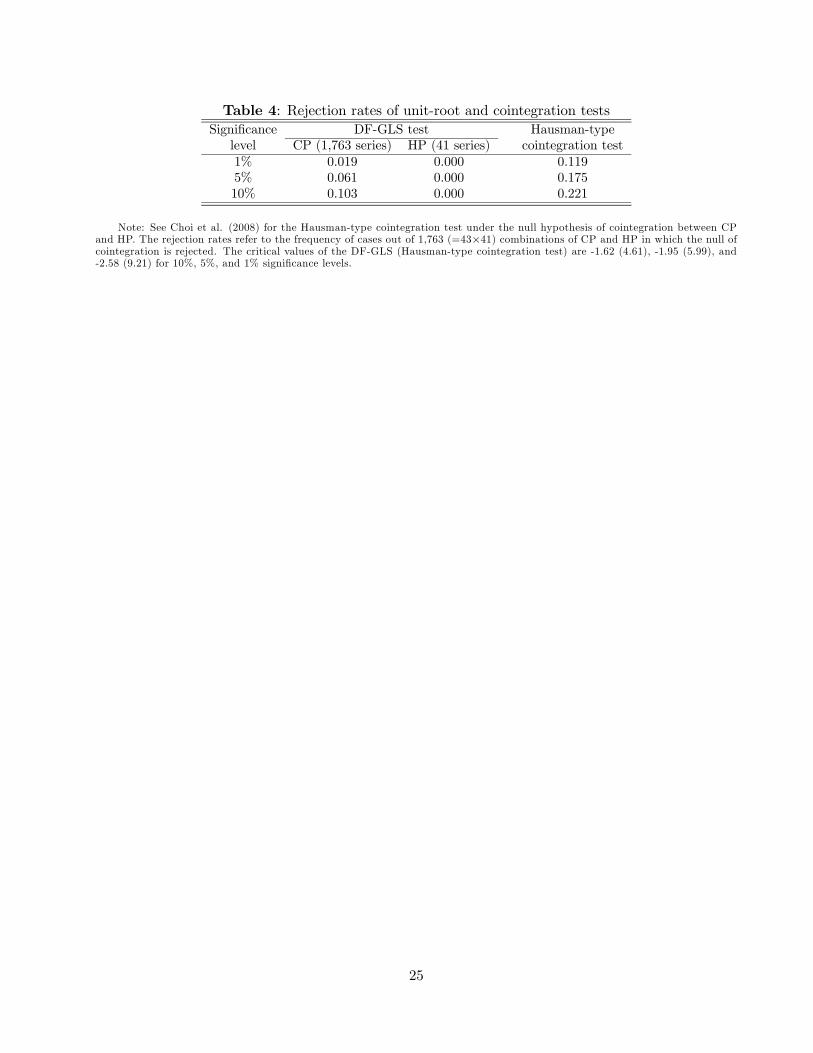
Table 4: Rejection rates of unit-root and cointegration tests

Significance DF-GLS test Hausman-type

level CP (1,763 series) HP (41 series) cointegration test

1% 0.019 0.000 0.119

5% 0.061 0.000 0.175

10% 0.103 0.000 0.221

Note: See Choi et al. (2008) for the Hausman-type cointegration test under the null hypothesis of cointegration between CPand HP. The rejection rates refer to the frequency of cases out of 1,763 (=43×41) combinations of CP and HP in which the null ofcointegration is rejected. The critical values of the DF-GLS (Hausman-type cointegration test) are -1.62 (4.61), -1.95 (5.99), and-2.58 (9.21) for 10%, 5%, and 1% significance levels.

25

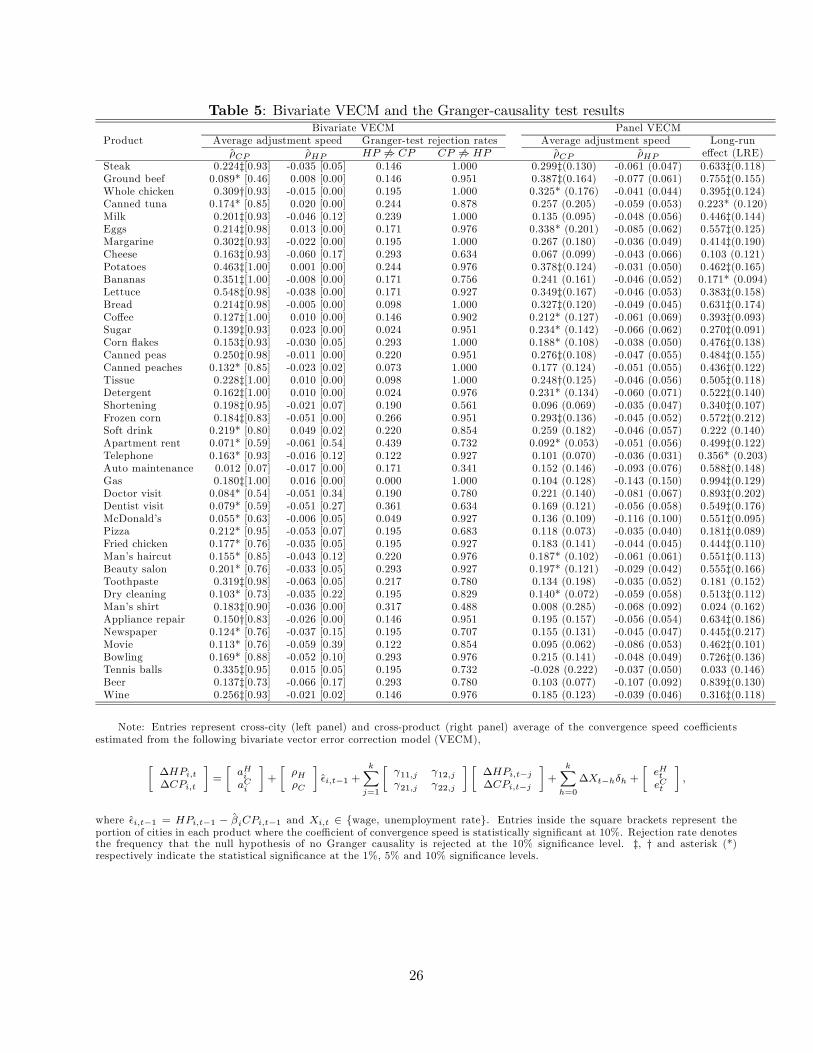
Table 5: Bivariate VECM and the Granger-causality test resultsBivariate VECM Panel VECM

Product Average adjustment speed Granger-test rejection rates Average adjustment speed Long-run

6⇒ 6⇒ effect (LRE)

Steak 0.224‡[0.93] -0.035 [0.05] 0.146 1.000 0.299‡(0.130) -0.061 (0.047) 0.633‡(0.118)Ground beef 0.089* [0.46] 0.008 [0.00] 0.146 0.951 0.387‡(0.164) -0.077 (0.061) 0.755‡(0.155)Whole chicken 0.309†[0.93] -0.015 [0.00] 0.195 1.000 0.325* (0.176) -0.041 (0.044) 0.395‡(0.124)Canned tuna 0.174* [0.85] 0.020 [0.00] 0.244 0.878 0.257 (0.205) -0.059 (0.053) 0.223* (0.120)

Milk 0.201‡[0.93] -0.046 [0.12] 0.239 1.000 0.135 (0.095) -0.048 (0.056) 0.446‡(0.144)Eggs 0.214‡[0.98] 0.013 [0.00] 0.171 0.976 0.338* (0.201) -0.085 (0.062) 0.557‡(0.125)Margarine 0.302‡[0.93] -0.022 [0.00] 0.195 1.000 0.267 (0.180) -0.036 (0.049) 0.414‡(0.190)Cheese 0.163‡[0.93] -0.060 [0.17] 0.293 0.634 0.067 (0.099) -0.043 (0.066) 0.103 (0.121)

Potatoes 0.463‡[1.00] 0.001 [0.00] 0.244 0.976 0.378‡(0.124) -0.031 (0.050) 0.462‡(0.165)Bananas 0.351‡[1.00] -0.008 [0.00] 0.171 0.756 0.241 (0.161) -0.046 (0.052) 0.171* (0.094)

Lettuce 0.548‡[0.98] -0.038 [0.00] 0.171 0.927 0.349‡(0.167) -0.046 (0.053) 0.383‡(0.158)Bread 0.214‡[0.98] -0.005 [0.00] 0.098 1.000 0.327‡(0.120) -0.049 (0.045) 0.631‡(0.174)Coffee 0.127‡[1.00] 0.010 [0.00] 0.146 0.902 0.212* (0.127) -0.061 (0.069) 0.393‡(0.093)Sugar 0.139‡[0.93] 0.023 [0.00] 0.024 0.951 0.234* (0.142) -0.066 (0.062) 0.270‡(0.091)Corn flakes 0.153‡[0.93] -0.030 [0.05] 0.293 1.000 0.188* (0.108) -0.038 (0.050) 0.476‡(0.138)Canned peas 0.250‡[0.98] -0.011 [0.00] 0.220 0.951 0.276‡(0.108) -0.047 (0.055) 0.484‡(0.155)Canned peaches 0.132* [0.85] -0.023 [0.02] 0.073 1.000 0.177 (0.124) -0.051 (0.055) 0.436‡(0.122)Tissue 0.228‡[1.00] 0.010 [0.00] 0.098 1.000 0.248†(0.125) -0.046 (0.056) 0.505‡(0.118)Detergent 0.162‡[1.00] 0.010 [0.00] 0.024 0.976 0.231* (0.134) -0.060 (0.071) 0.522‡(0.140)Shortening 0.198‡[0.95] -0.021 [0.07] 0.190 0.561 0.096 (0.069) -0.035 (0.047) 0.340‡(0.107)Frozen corn 0.184‡[0.83] -0.051 [0.00] 0.266 0.951 0.293‡(0.136) -0.045 (0.052) 0.572‡(0.212)Soft drink 0.219* [0.80] 0.049 [0.02] 0.220 0.854 0.259 (0.182) -0.046 (0.057) 0.222 (0.140)

Apartment rent 0.071* [0.59] -0.061 [0.54] 0.439 0.732 0.092* (0.053) -0.051 (0.056) 0.499‡(0.122)Telephone 0.163* [0.93] -0.016 [0.12] 0.122 0.927 0.101 (0.070) -0.036 (0.031) 0.356* (0.203)

Auto maintenance 0.012 [0.07] -0.017 [0.00] 0.171 0.341 0.152 (0.146) -0.093 (0.076) 0.588‡(0.148)Gas 0.180‡[1.00] 0.016 [0.00] 0.000 1.000 0.104 (0.128) -0.143 (0.150) 0.994‡(0.129)Doctor visit 0.084* [0.54] -0.051 [0.34] 0.190 0.780 0.221 (0.140) -0.081 (0.067) 0.893‡(0.202)Dentist visit 0.079* [0.59] -0.051 [0.27] 0.361 0.634 0.169 (0.121) -0.056 (0.058) 0.549‡(0.176)McDonald’s 0.055* [0.63] -0.006 [0.05] 0.049 0.927 0.136 (0.109) -0.116 (0.100) 0.551‡(0.095)Pizza 0.212* [0.95] -0.053 [0.07] 0.195 0.683 0.118 (0.073) -0.035 (0.040) 0.181‡(0.089)Fried chicken 0.177* [0.76] -0.035 [0.05] 0.195 0.927 0.183 (0.141) -0.044 (0.045) 0.444‡(0.110)Man’s haircut 0.155* [0.85] -0.043 [0.12] 0.220 0.976 0.187* (0.102) -0.061 (0.061) 0.551‡(0.113)Beauty salon 0.201* [0.76] -0.033 [0.05] 0.293 0.927 0.197* (0.121) -0.029 (0.042) 0.555‡(0.166)Toothpaste 0.319‡[0.98] -0.063 [0.05] 0.217 0.780 0.134 (0.198) -0.035 (0.052) 0.181 (0.152)

Dry cleaning 0.103* [0.73] -0.035 [0.22] 0.195 0.829 0.140* (0.072) -0.059 (0.058) 0.513‡(0.112)Man’s shirt 0.183‡[0.90] -0.036 [0.00] 0.317 0.488 0.008 (0.285) -0.068 (0.092) 0.024 (0.162)

Appliance repair 0.150†[0.83] -0.026 [0.00] 0.146 0.951 0.195 (0.157) -0.056 (0.054) 0.634‡(0.186)Newspaper 0.124* [0.76] -0.037 [0.15] 0.195 0.707 0.155 (0.131) -0.045 (0.047) 0.445‡(0.217)Movie 0.113* [0.76] -0.059 [0.39] 0.122 0.854 0.095 (0.062) -0.086 (0.053) 0.462‡(0.101)Bowling 0.169* [0.88] -0.052 [0.10] 0.293 0.976 0.215 (0.141) -0.048 (0.049) 0.726‡(0.136)Tennis balls 0.335‡[0.95] 0.015 [0.05] 0.195 0.732 -0.028 (0.222) -0.037 (0.050) 0.033 (0.146)

Beer 0.137‡[0.73] -0.066 [0.17] 0.293 0.780 0.103 (0.077) -0.107 (0.092) 0.839‡(0.130)Wine 0.256‡[0.93] -0.021 [0.02] 0.146 0.976 0.185 (0.123) -0.039 (0.046) 0.316‡(0.118)

Note: Entries represent cross-city (left panel) and cross-product (right panel) average of the convergence speed coefficients

estimated from the following bivariate vector error correction model (VECM),

∆∆

=

+

−1 +

=1

11 1221 22

∆−∆−

+

=0

∆− +

where −1 = −1 − −1 and ∈ {wage, unemployment rate}. Entries inside the square brackets represent theportion of cities in each product where the coefficient of convergence speed is statistically significant at 10%. Rejection rate denotesthe frequency that the null hypothesis of no Granger causality is rejected at the 10% significance level. ‡, † and asterisk (*)respectively indicate the statistical significance at the 1%, 5% and 10% significance levels.

26

Table 6: Transmission mechanisms and the related variablesTransmission Variables (expected signs)

mechanism City characteristics Product characteristics

Wealth effect Per capita income (−) Price flexibility (+)

Share of college graduates (−)Demand-pull Homeownership rate (+)

channel

Collateral effect Financial integration (+) Price flexibility (+)

Share of college graduates (−)Homeownership rate (+)

. . . . . . . . . . . . . . . . . . . . . . . . . . . . . . . . . . . . . . . . . . . . . . . . . . . . . . . . . . . . . . . . . . . . . . . . . . . . . . . . . . . . . . . . . . . . . . .

Markup effect Population density (−) Production proximity (−)Remoteness (+) Price flexibility (−)

Cost-push Unemployment rate (−)channel Homeownership rate (+)

Local cost effect Housing supply constraint (+) Production proximity (+)

Note: Signs inside the parenthesis represent the expected signs of variables to support the corresponding effect.

27

Table 7: Regression results for the transmission mechanism of aggregate housing demand andsupply shocks

Explanatory Variables contemporaneous After 1 year After 2 years After 3 years After 4 years

Housing demand shock

Constant -0.053 [0.064] -0.190 [0.169] -0.001 [0.198] 0.164 [0.244] 0.257 [0.274]

Dummy for Most FLEX gp 0.024‡[0.011] 0.079* [0.042] 0.123†[0.061] 0.153†[0.073] 0.166‡[0.078]Dummy for Med FLEX gp 0.011 [0.015] 0.030 [0.044] 0.046 [0.059] 0.070 [0.072] 0.084 [0.079]

Per capita income 0.001 [0.001] 0.000 [0.003] -0.005 [0.004] -0.007 [0.005] -0.009 [0.006]

Population Density 0.001 [0.001] 0.002 [0.003] 0.004 [0.005] 0.008 [0.006] 0.010 [0.007]

Share of skilled worker 0.001* [0.001] 0.004†[0.002] 0.005†[0.002] 0.005‡[0.002] 0.005‡[0.002]Remoteness -0.007 [0.014] 0.005 [0.040] 0.044 [0.054] 0.075 [0.067] 0.093 [0.075]

Unemployment rate 0.005 [0.004] 0.012 [0.010] 0.004 [0.013] -0.006 [0.015] -0.013 [0.017]

Financial integration 0.015 [0.011] 0.028 [0.031] 0.051 [0.040] 0.055 [0.048] 0.053 [0.054]

Homeownership rate -0.111* [0.057] -0.188 [0.169] -0.312 [0.195] -0.425* [0.225] -0.441* [0.247]

Housing supply constraint 0.034†[0.015] 0.094‡[0.033] 0.094 [0.043] 0.088* [0.052] 0.085 [0.059]

Housing supply shock

Constant -0.158 [0.175] -0.586‡[0.287] -0.632‡[0.273] -0.619‡[0.279] -0.595‡[0.275]Dummy for LOCAL group 0.106‡[0.047] 0.119* [0.066] 0.133* [0.076] 0.151* [0.078] 0.161†[0.077]Dummy for MAYBE LOCAL 0.017 [0.030] 0.084* [0.050] 0.093 [0.059] 0.104* [0.062] 0.113* [0.064]

Per capita income -0.008‡[0.004] -0.003 [0.005] -0.004 [0.005] -0.004 [0.005] -0.005 [0.005]

Population Density -0.004 [0.004] -0.002 [0.006] -0.003 [0.007] -0.002 [0.007] -0.001 [0.007]

Share of skilled worker 0.001 [0.002] 0.004 [0.003] 0.005 [0.003] 0.005* [0.003] 0.005* [0.003]

Remoteness -0.006 [0.042] -0.087‡[0.053] -0.098 [0.067] -0.092 [0.067] -0.085 [0.065]

Unemployment rate 0.000 [0.011] 0.016 [0.015] 0.018 [0.017] 0.016 [0.018] 0.015 [0.017]

Financial integration -0.013 [0.041] -0.041 [0.053] -0.033 [0.063] -0.030 [0.064] -0.028 [0.062]

Homeownership rate 0.456‡[0.162] 0.541‡[0.368] 0.568†[0.284] 0.534* [0.291] 0.521* [0.290]

Housing supply constraint 0.065* [0.039] 0.187‡[0.058] 0.214‡[0.062] 0.221‡[0.061] 0.225‡[0.060]

Note: The regression equation is

= +

2=1

+0 + for = 1 43 = 1 41 = 0 4

where

represents the h-year median cumulative effect of housing market shocks on the price of the product in city .

denotes a product dummy variable. For the house demand shock, 1 and 2 respectively represent dummy variables for themost flexible price group (Most FLEX) and less-flexible price group (Med FLEX) by setting the least flexible price group as thebase group. For the house supply shock, 1 and 2 respectively denote dummy variables for the locally produced product group(LOCAL) and maybe locally produced product group (MAYBE LOCAL) by setting the not locally produced product group asthe base group. is a set of city-level characteristics including per capita income, population density, share of college graduates,remoteness, unemployment rate, financial integration, homeownership and the housing supply constraint by Guren et al. (2020).Clustered standard errors are used by clustering observations by cities rather than by products. ‡, † and asterisk (*) respectivelyindicate the statistical significance at the 1%, 5% and 10% significance levels.

28

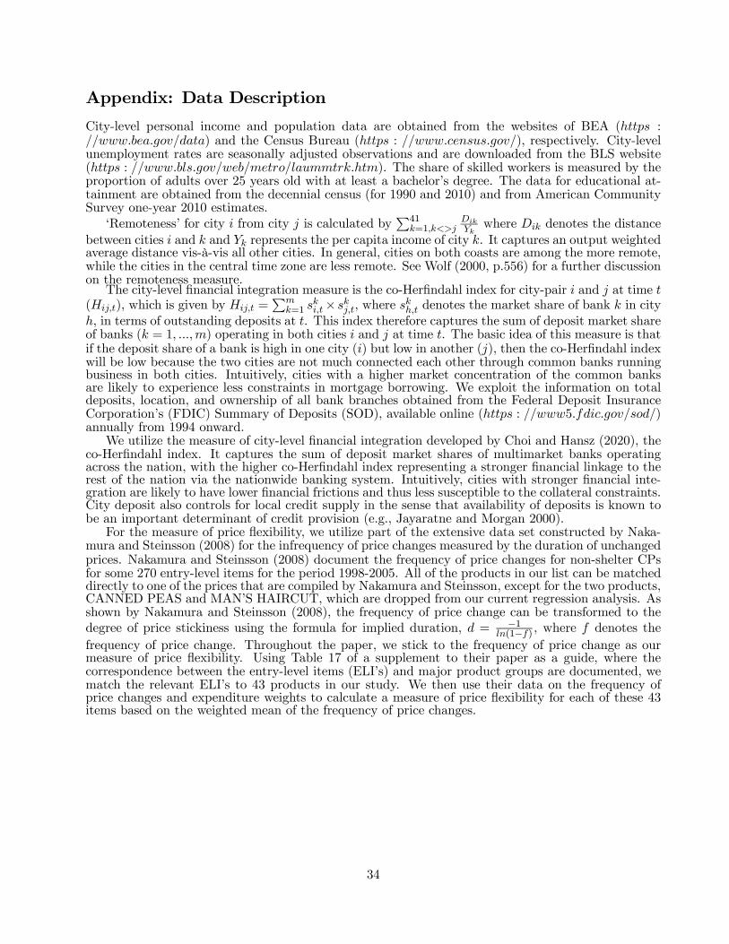
Appendix: Data Description

City-level personal income and population data are obtained from the websites of BEA ( :) and the Census Bureau ( : ), respectively. City-levelunemployment rates are seasonally adjusted observations and are downloaded from the BLS website( : ). The share of skilled workers is measured by theproportion of adults over 25 years old with at least a bachelor’s degree. The data for educational at-tainment are obtained from the decennial census (for 1990 and 2010) and from American CommunitySurvey one-year 2010 estimates.

‘Remoteness’ for city from city is calculated byP41

=1

where denotes the distance

between cities and and represents the per capita income of city . It captures an output weightedaverage distance vis-à-vis all other cities. In general, cities on both coasts are among the more remote,while the cities in the central time zone are less remote. See Wolf (2000, p.556) for a further discussionon the remoteness measure.

The city-level financial integration measure is the co-Herfindahl index for city-pair and at time (), which is given by =

P=1

× , where

denotes the market share of bank in city

, in terms of outstanding deposits at . This index therefore captures the sum of deposit market shareof banks ( = 1 ) operating in both cities and at time . The basic idea of this measure is thatif the deposit share of a bank is high in one city () but low in another (), then the co-Herfindahl indexwill be low because the two cities are not much connected each other through common banks runningbusiness in both cities. Intuitively, cities with a higher market concentration of the common banksare likely to experience less constraints in mortgage borrowing. We exploit the information on totaldeposits, location, and ownership of all bank branches obtained from the Federal Deposit InsuranceCorporation’s (FDIC) Summary of Deposits (SOD), available online ( : 5)annually from 1994 onward.

We utilize the measure of city-level financial integration developed by Choi and Hansz (2020), theco-Herfindahl index. It captures the sum of deposit market shares of multimarket banks operatingacross the nation, with the higher co-Herfindahl index representing a stronger financial linkage to therest of the nation via the nationwide banking system. Intuitively, cities with stronger financial inte-gration are likely to have lower financial frictions and thus less susceptible to the collateral constraints.City deposit also controls for local credit supply in the sense that availability of deposits is known tobe an important determinant of credit provision (e.g., Jayaratne and Morgan 2000).

For the measure of price flexibility, we utilize part of the extensive data set constructed by Naka-mura and Steinsson (2008) for the infrequency of price changes measured by the duration of unchangedprices. Nakamura and Steinsson (2008) document the frequency of price changes for non-shelter CPsfor some 270 entry-level items for the period 1998-2005. All of the products in our list can be matcheddirectly to one of the prices that are compiled by Nakamura and Steinsson, except for the two products,CANNED PEAS and MAN’S HAIRCUT, which are dropped from our current regression analysis. Asshown by Nakamura and Steinsson (2008), the frequency of price change can be transformed to the

degree of price stickiness using the formula for implied duration, = −1(1−) , where denotes the

frequency of price change. Throughout the paper, we stick to the frequency of price change as ourmeasure of price flexibility. Using Table 17 of a supplement to their paper as a guide, where thecorrespondence between the entry-level items (ELI’s) and major product groups are documented, wematch the relevant ELI’s to 43 products in our study. We then use their data on the frequency ofprice changes and expenditure weights to calculate a measure of price flexibility for each of these 43items based on the weighted mean of the frequency of price changes.

34

Table A.1: Data Description (by product)

No. Item G1 G2 Descriptions

1 Steak H B Pound, USDA Choice

2 Ground beef H B Pound, lowest price

3 Whole chicken H B Pound, whole fryer

4 Canned tuna M B Starkist or Chicken of the Sea; 6.5 oz.(85.1-91.3),6.125 oz.(91.4-95.3),

6-6.125 oz.(95.3-99.4), 6.0 oz. (00.1-09.4)

5 Milk H B 1/2 gal. carton

6 Eggs H B One Dozen, Grade A, Large

7 Margarine H B One Pound, Blue Bonnet or Parkay

8 Cheese H A Parmesan, grated 8 oz. canister, Kraft

9 Potatoes H B 10 lbs. white or red

10 Bananas M A One pound

11 Lettuce H B Head, approximately 1.25 pounds

12 Bread M B 24 oz loaf

13 Coffee M A Can, Maxwell House, Hills Brothers, or Folgers; 1 lb. (85.1-88.3); 13 oz. (88.4-99.4);

11.5 oz. (00.1-09.4)

14 Sugar M B Cane or beet; 5 lbs. (85.1-92.3); 4 lbs. (92.4-09.4)

15 Corn flakes M A 18 oz, Kellog’s or Post Toasties

16 Canned peas - A Can, Del Monte or Green Giant; 17 oz can, 15-17 oz. (85.1-85.4), 17 oz. (86.1-91.4),

15-15.25 oz. (92.1-09.4)

17 Canned peaches M A 1/2 can approx. 29 oz.; Hunt’s, Del Monte, or Libby’s or Lady Alberta

18 Tissue L A 175-count box (85.1-02.3), 200-count box (02.4-09.4); Kleenex brand

19 Detergent M A 42 oz, Tide, Bold, or Cheer (85.1-96.3); 50 oz. (96.4-00.4), 60 oz (01.1-02.3),

75 oz (02.4-09.4), Cascade dishwashing powder

20 Shortening M A 3 lbs. can, all-vegetable, Crisco brand

21 Frozen corn M A 10 oz. (85.1-95.3), 16 oz. (95.4-09.4); Whole Kernel

22 Soft drink M A 2 liter Coca Cola

23 Apartment rent H C 2-Bedroom, unfurnished, excld. all utilities except water, 1.2 or 2 baths, approx. 950 sqft

24 Home price - C 1,800 sqft, new house, 8,000 sqft lot, (85.1-99.4);

2,400 sqft, new house, 8,000 sqft lot, 4 bedrooms, 2 baths (00.1-09.4)

25 Telephone M C Private residential line, basic monthly rate, fees and taxes

26 Auto maintenance M C average price to balance one front wheel (85.1-88.3);

average price to computer or spin balance one front wheel (88.4-09.4)

27 Gas H A One gallon regular unleaded, national brand, including all taxes

28 Doctor visit L C General practitioner’s routine examination of established patient

29 Dentist visit L C Adult teeth cleaning and periodic oral exam (85.1-04.4); Adult teeth cleaning (05.1-09.1)

30 McDonald’s L C McDonald’s Quarter-Pounder with Cheese

31 Pizza M C 12"-13" (85.1-94.3), 11"-12" (94.4-09.4) thin crust cheese pizza,

Pizza Hut or Pizza Inn from 1990Q1 to 1994Q3

32 Fried chicken M C Thigh and Drumstick, KFC or Church’s where available

33 Man’s haircut L C Man’s barber shop haircut, no styling

34 Beauty salon L C Woman’s shampoo, trim, and blow dry

35 Toothpaste L A 6 to 7 oz. tube (85.1-06.2), 6 oz-6.4oz tube (06.3-09.4); Crest, or Colgate

36 Dry cleaning L C Man’s two-piece suit

37 Man’s shirt L A Arrow, Enro, Van Huesen, or JC Penny’s Stafford, White, cotton/polyester blend

(at least 55% cotton) long sleeves (85.1-94.3); 100% cotton pinpoint Oxford,

Long sleeves (94.4-99.4)Cotton/Polyester, pinpoint weave, long sleeves (00.1-09.4)

38 Appliance repair M C Home service call, washing machine, excluding parts

39 Newspaper L C Daily and Sunday home delivery, large-city newspaper, monthly rate

40 Movie M C First-run, indoor, evening, no discount

41 Bowling L C Price per line, evening rate (85.1-98.2); Saturday evening non-league rate (98.3-09.4)

42 Tennis balls L A Can of three extra duty, yellow, Wilson or Penn Brand

43 Beer M A 6-pack, 12 oz containers, excluding deposit; Budweiser or Miller Lite, (85.1-99.4),

Heineken’s (00.1-09.4)

44 Wine L A 1.5-liter bottle; Paul Masson Chablis (85.1-90.3)

Gallo sauvignon blanc (90.4-91.3), Gallo chablis blanc (91.4-97.3)

Livingston Cellars or Gallo chablis blanc (97.1-00.1)

Livingston Cellars or Gallo chablis or Chenin blanc (00.2-09.4)

Notes: ‘G1’ denotes three product groups based on the degree of price flexibility: highly flexible (H), medium flexible(M), and less flexible (L). ‘G2’ denotes three product groups based on the proximity of production to the market place:not locally produced (A), maybe locally produced (B), and locally produced goods and services (C).

35

Table A.2: Summary statistics

Product Price level % deviation from

mean min max ratio(%) Dispersion Moran’s city average price

(CV) I [min,max]

Steak 6.22 5.45 7.20 32.1 0.07 0.175 [-0.12, 0.16]

Ground beef 1.71 1.37 2.05 49.6 0.08 0.056 [-0.21, 0.17]

Whole chicken 0.90 0.76 1.16 52.6 0.13 0.074 [-0.17, 0.23]

Canned tuna 0.71 0.60 0.93 55.0 0.10 0.066 [-0.16, 0.26]

Milk 1.57 1.33 1.82 36.8 0.08 0.145 [-0.14, 0.13]

Eggs 1.04 0.84 1.81 115.5 0.18 0.377 [-0.15, 0.52]

Margarine 0.70 0.60 1.12 86.7 0.14 0.071 [-0.17, 0.41]

Cheese 3.34 2.94 4.09 39.1 0.08 0.100 [-0.11, 0.17]

Potatoes 2.71 1.92 3.47 80.7 0.14 0.289 [-0.29, 0.24]

Bananas 0.48 0.39 0.61 56.4 0.10 0.172 [-0.21, 0.21]

Lettuce 1.01 0.86 1.27 47.7 0.09 0.278 [-0.19, 0.24]

Bread 0.86 0.65 1.14 75.4 0.13 0.036 [-0.25, 0.26]

Coffee 2.83 2.51 3.56 41.8 0.10 0.274 [-0.13, 0.22]

Sugar 1.63 1.37 1.92 40.1 0.06 0.083 [-0.15, 0.15]

Corn flakes 2.28 1.95 2.67 36.9 0.09 0.061 [-0.10, 0.12]

Canned peas 0.68 0.57 0.84 47.4 0.10 0.174 [-0.19, 0.20]

Canned peaches 1.50 1.34 1.84 37.3 0.07 0.063 [-0.13, 0.13]

Tissue 1.26 1.12 1.52 35.7 0.07 0.134 [-0.10, 0.17]

Detergent 3.21 2.89 3.78 30.8 0.07 0.128 [-0.11, 0.13]

Shortening 2.90 2.49 3.37 35.3 0.07 0.141 [-0.14, 0.14]

Frozen corn 0.92 0.80 1.11 38.8 0.08 0.051 [-0.15, 0.17]

Soft drink 1.23 1.05 1.45 38.1 0.08 0.023 [-0.15, 0.13]

Apartment rent 580.38 432.97 1,067.89 146.6 0.19 0.097 [-0.30, 0.62]

Home Price 165.17 133.56 371.55 178.2 0.23 0.119 [-0.16, 0.70]

Telephone 20.85 15.55 29.88 92.2 0.15 0.069 [-0.28, 0.22]

Auto maintenance 7.44 5.41 8.89 64.3 0.09 0.016 [-0.29, 0.11]

Gas 1.45 1.35 1.61 19.3 0.04 0.659 [-0.07, 0.10]

Doctor visit 50.95 42.15 61.43 45.7 0.09 0.073 [-0.18, 0.16]

Dentist visit 58.65 47.78 93.69 96.1 0.14 0.079 [-0.22, 0.41]

McDonald’s 2.05 1.91 2.20 15.2 0.03 0.147 [-0.06, 0.07]

Pizza 8.84 8.12 10.27 26.5 0.05 0.042 [-0.08, 0.10]

Fried chicken 2.37 1.98 2.77 39.9 0.08 0.030 [-0.19, 0.16]

Man’s haircut 9.18 7.31 11.64 59.2 0.11 0.013 [-0.21, 0.23]

Beauty salon 23.14 16.78 31.36 86.9 0.14 0.017 [-0.36, 0.27]

Toothpaste 2.07 1.71 2.42 41.5 0.07 0.041 [-0.17, 0.17]

Dry cleaning 6.98 5.64 8.42 49.3 0.11 0.058 [-0.23, 0.19]

Man’s shirt 24.78 22.69 30.05 32.4 0.06 0.049 [-0.16, 0.20]

Appliance repair 37.80 25.95 48.14 85.5 0.11 0.030 [-0.40, 0.22]

Newspaper 12.00 7.13 16.75 134.9 0.18 0.039 [-0.36, 0.27]

Movie 6.39 5.72 7.95 39.0 0.07 0.117 [-0.09, 0.24]

Bowling 2.54 1.82 3.22 76.9 0.13 0.060 [-0.28, 0.23]

Tennis balls 2.34 2.02 2.96 46.5 0.08 0.010 [-0.14, 0.26]

Beer 5.28 4.83 6.33 31.1 0.05 0.048 [-0.10, 0.15]

Wine 5.56 4.40 6.79 54.3 0.10 0.050 [-0.21, 0.17]

Note: Entries represent mean, volatiltiy (CV), minimum, and maximum of average annual prices in dollar, except for“Home Price” which is in thousand dollars. ‘Ratio’ denotes the ratio of the highest price to the lowest price in percent.‘affordability’ represents CPs divided by annual wage or income. ‘Moran’s I statistics is a measure of the co-movementsof city-level price series using the following modified Moran’s I statistic.

36

Table A.3: Summary statistics at the city level

city City name Income Population Share of Home price House supply Homeowner-

code (CODE) ($) (1,000 ppl) skilled ($1,000) elasticity ship rate (%)

1 AMARILLO, TX (AMA) 24,933 225.7 21.9 166.9 0.489 64.1

2 ATLANTA, GA (ATL) 29,895 4,124.2 34.0 189.0 1.049 63.3

3 CEDAR RAPIDS, IA (CID) 28,688 234.0 26.6 174.4 0.681 74.7

4 CHARLOTTE, NC (CLT) 28,281 1,720.9 31.7 175.2 0.619 65.3

5 CHATTANOOGA, TN (CHA) 25,707 476.7 22.4 170.6 0.525 67.2

6 CLEVELAND, OH (CLE) 30,168 2,116.9 26.3 186.4 0.533 65.1

7 COLORADO SPRINGS, CO (COS) 28,253 525.7 34.8 190.3 0.288 63.5

8 COLUMBIA, MO (COU) 26,777 135.4 43.3 173.0 0.594 55.5

9 COLUMBIA, SC (CAE) 25,843 646.1 29.9 164.9 0.490 67.2

10 DALLAS, TX (DAL) 30,870 5,122.2 30.1 157.7 0.652 59.9

11 DENVER, CO (DEN) 34,063 2,099.7 37.1 231.4 0.410 63.4

12 DOVER, DE (DOV) 24,721 131.6 19.4 184.2 - 70.0

13 HOUSTON, TX (HOU) 31,677 4,724.4 28.1 155.6 0.738 60.4

14 HUNTSVILLE, AL (HSV) 27,952 346.3 34.1 164.3 0.350 69.5

15 JONESBORO, AR (JBR) 21,746 106.2 19.6 156.7 0.312 58.7

16 JOPLIN, MO (JLN) 22,405 154.4 18.1 156.8 0.527 67.0

17 KNOXVILLE, TN (KNX*) 25,157 741.9 27.8 163.9 0.568 68.1

18 LEXINGTON, KY (LEX) 28,076 405.3 33.4 174.2 0.522 58.7

19 LOS ANGELES, CA (LAX) 31,459 12,057.1 30.0 409.3 1.189 48.5

20 LOUISVILLE, KY (LOU*) 27,928 1,121.3 23.8 162.5 0.522 67.1

21 LUBBOCK, TX (LBB) 24,009 260.4 26.3 156.2 0.403 56.4

22 MEMPHIS, TN (MEM) 27,632 1,195.0 24.4 153.5 0.551 60.7

23 MONTGOMERY, AL (MGM) 26,111 340.4 26.2 182.9 0.515 64.8

24 ODESSA, TX (ODS*) 23,000 126.9 13.0 167.4 0.585 65.4

25 OKLAHOMA CITY, OK (OKC) 27,121 1,101.9 27.0 159.2 0.669 64.1

26 OMAHA, NE (OMA) 30,860 766.7 31.3 163.7 0.628 65.6

27 PHILADELPHIA, PA (PHL) 33,571 5,678.2 31.8 270.2 0.905 67.2

28 PHOENIX, AZ (PHX) 27,280 3,163.3 27.3 189.5 0.946 61.9

29 PORTLAND, OR (POR*) 29,594 1,869.5 32.9 244.5 0.613 61.2

30 RALEIGH, NC (RDU) 30,653 799.9 41.3 186.3 0.415 65.7

31 RENO-SPARKS, NV (RNO) 33,645 336.6 26.3 214.2 1.153 57.5

32 SALT LAKE CITY, UT (SLC) 26,507 918.9 29.8 190.6 0.314 67.1

33 SAN ANTONIO, TX (SAT) 25,538 1,729.8 24.5 163.8 0.670 62.2

34 SOUTH BEND, IN (SBN) 25,736 309.8 24.1 169.8 0.743 70.3

35 SPRINGFIELD, IL (SPI) 29,162 200.8 29.6 172.3 0.530 69.9

36 ST. CLOUD, MN (STC) 24,374 166.8 22.4 169.2 1.071 69.8

37 ST. LOUIS, MO (STL) 30,428 2,667.5 28.5 161.9 0.921 69.3

38 TACOMA, WA (SEA) 35,396 2,966.6 36.7 206.5 0.676 59.8

39 TUCSON, AZ (TUS) 24,845 819.9 29.0 179.7 0.752 61.9

40 WACO, TX (WAC*) 22,662 228.9 20.4 155.6 0.566 59.4

41 YORK, PA (YRK*) 27,903 381.8 21.0 196.4 0.521 74.6

. . . . . . . . . . . . . . . . . . . . . . . . . . . . . . . . . . . . . . . . . . . . . . . . . . . . . . . . . . . . . . . . . . . . . . . . . . . . . . . . . . . . . . . . . . . . . . . . . . . . . . . . . . . . . . . . . . . . . . . . . . . . .

Average 27,820 1,542.6 28.0 184.4 0.642 64.2

Note: ‘Share of skilled’ represents the fraction of adult population who got at least bachelor’s degree. City codes arethe airport codes of the corresponding cities except for those asterisked.

37

Table A.4: Description of city-level and product-level characteristics

Variable Description Source

Income Per capita personal income of the U.S. Metropolitan BEA website

area during 1990-2016

Population Average population density of the U.S. Metropolitan Census Bureau website

area during 1990-2016

Homeownership Average fraction of the owner-occupied houses out Census Bureau website

rate of the entire occupied housing units during 2000-2018

Unemployment Average city-level unemployment rate (s.a.) BLS website

rate over 1990-2016

Share of Share of adults over 25 years old with at least Census Bureau website

skilled worker a bachelor’s degree (1990-2016)

Remoteness City-level remoteness measure by Wolf (2000) Authors’ computation

over 1990-2016

Financial Annual total deposits by the all branches of all Summary of Deposits

Integration insured banks during 1994-2017 at the FDIC website

Housing supply City-level housing supply elasticities based on Guren’s website

elasticity the systematic historical sensitivity of local house

prices to regional housing cycles

. . . . . . . . . . . . . . . . . . . . . . . . . . . . . . . . . . . . . . . . . . . . . . . . . . . . . . . . . . . . . . . . . . . . . . . . . . . . . . . . . . . . . . . . . . . . . . . . . . . .

Price The frequency of price changed and expenditure Nakamura and Steinsson

flexibility weights for 43 products for the period 1998-2005 (2008), Table 17

Production The proximity of production to the market place O’Connell and Wei (2002)

proximity

38

(a) Nominal per capita income

(b) Population

Figure 1: Income and population of the U.S. Cities

Note: The figure maps the location of each city and the size of the circle denotes the size of the city

in terms of per capita income (top) and population (bottom).

29

11 11.5 12 12.5 13 13.5House prices (logs)

4.8

5

5.2

5.4

5.6

5.8

6

6.2

6.4

11 11.5 12 12.5 13 13.5

House prices (logs)

6.2

6.4

6.6

6.8

7

7.2

7.4

7.6

7.8

8

(a) log HP and log price of cornflakes (b) log HP and log price of haircuts

-0.2 -0.1 0 0.1 0.2 0.3 0.4 0.5 0.6 0.7 0.8

House prices (logs)

-0.4

-0.3

-0.2

-0.1

0

0.1

0.2

0.3

0.4

-0.2 -0.1 0 0.1 0.2 0.3 0.4 0.5 0.6 0.7 0.8

House prices (logs)

-0.3

-0.2

-0.1

0

0.1

0.2

0.3

0.4

(c) growth rates of HP and cornflake price (d) growth rates of HP and haircut price

Figure 2: Relationship between annual average HP and CP (on the top panel) and

relationship between growth rates of HP and CP (on the bottom panel)

Note: This figure displays the relationship between annualized HP and the price of ‘CORNFLAKE’

(top-left panel) and price of ‘HAIRCUT’ (top-right panel), and the relationship between annualized HP

growth and the growth rates of ‘CORNFLAKE’ (bottom-left panel) and growth rates of ‘HAIRCUT’

(bottom-right panel).

30

0 2 4 6 8 10 12 14 16 18

quarters

0

0.2

0.4

0.6

0.8

1

1.2

1.4

1.6

1.8

2

(a) Response of local HP to the aggregate housing demand shock

0 2 4 6 8 10 12 14 16 18

quarters

-0.6

-0.5

-0.4

-0.3

-0.2

-0.1

0

0.1

0.2

0.3

(b) Response of local HP to the aggregate housing supply shock

Figure 3: Responses of local HP to aggregate housing market shocks

Note: This figure plots the cumulative IRFs of local HP in 41 cities to aggregate housing demand

and supply shocks on the top and bottom panes, respectively. The solid line represents the median

response among the 41 cities, and the dashed lines are the inter-city quartile (25- and 75-percentile)

bands.

31

(a) Relationship between price flexibility and adjustment speed

(b) Relationship between price flexibility and long-run effect

Figure 4: Degree of price flexibility and average adjustment speed and

long-run effect estimated from the (P)VECM

Note: The top panel shows the relationship between price flexibility and the adjustment speed of

CP to the deviation from long-run equilibrium across 43 products, estimated from VECM. The top

panel plots the relationship between price flexibility and the long-run effects of HP to CP among 43

products, estimated from the panel VECM.

32

Figure 5: The mean (solid line) and inter-quartiles (dotted lines) of long-run effect (LRE)

estimates of HP to CP for 10-year rolling window

Note: This figure plots the mean (solid line) and interquartile ranges (dotted lines) of the long-run

effects among 43 products, estimated from the Panel VECM using a 10-year rolling window.

33