Do Local Energy Prices and Regulation Affect the Geographic Concentration of Employment?

Matthew E. Kahn and Erin T. Mansur*

January 14, 2013

Abstract

Manufacturing industries differ with respect to their energy intensity, labor-to-capital ratio and their pollution intensity. Across the United States, there is significant variation in electricity prices and labor and environmental regulation. This paper examines whether the basic logic of comparative advantage can explain the geographical clustering of U.S. manufacturing. We document that energy-intensive industries concentrate in low electricity price counties and labor-intensive industries avoid pro-union counties. We find mixed evidence that pollution-intensive industries locate in counties featuring relatively lax Clean Air Act regulation.

* Kahn: UCLA and NBER. Institute of the Environment, La Kretz Hall, Suite 300, 619 Charles E. Young Drive East, Box 951496, Los Angeles, CA 90095. mkahn@ioe.ucla.edu. Mansur: Dartmouth College and NBER. Department of Economics, 6106 Rockefeller Hall, Hanover, NH 03755. erin.mansur@dartmouth.edu. We thank Severin Borenstein, Joseph Cullen, Lucas Davis, Meredith Fowlie, Jun Ishii, Enrico Moretti, Nina Pavcnik, Frank Wolak, Catherine Wolfram, and seminar participants at the 2009 UCEI Summer Camp, UBC Environmental Economics and Climate Change Workshop 2010, the 2012 UC Berkeley Power Conference, Claremont-McKenna College, Amherst College, the University of Alberta, the University of Michigan, and Yale University for useful comments. We thank Wayne Gray for sharing data with us and Koichiro Ito and William Bishop for assistance with Figure 1. We thank two anonymous reviewers for several useful comments.

1

1. Introduction

Between 1998 and 2009, aggregate U.S. manufacturing jobs declined by 35 percent while

the total production of this industry grew by 21 percent.1 This loss of manufacturing jobs has

important implications for the quality of life of the middle class. Manufacturing offers less

educated workers employment in relatively well paying jobs (Neal 1995). Despite public

concerns about the international outsourcing of jobs, over eleven million people continue to work

in the U.S. manufacturing sector.2 The ability of local areas to attract and retain such

manufacturing jobs continues to play an important role in determining the vibrancy of their local

economy (Greenstone, Hornbeck and Moretti 2010).

Ongoing research examines the role that government regulations and local factor prices

play in attracting or deflecting manufacturing employment. During a time when unemployment

rates differ greatly across states, there remains an open question concerning the role that

regulation plays in determining the geography of productive activity. A leading example of this

research is Holmes’ (1998) study that exploited sharp changes in labor regulation at adjacent

state boundaries. He posited that counties that are located in Right-to-Work states have a more

“pro-business” environment than their nearby neighboring county located in a pro-union state.

He used this border-pairs approach to establish that between 1952 and 1988 there has been an

increasing concentration of manufacturing activity on the Right-to-Work side of the border. A

1 The US Bureau of Labor Statistics reports employment by sector. From 1998 to 2009, manufacturing employment fell from 17.6 million to 11.5 million (http://data.bls.gov/timeseries/CES3000000001?data_tool=XGtable). The United Nations Statistics division reports gross value added by kind of economic activity at constant (2005) US dollars. From 1998 to 2009, manufacturing value went from $1348 billion to $1626 billion (http://data.un.org/Data.aspx?d=SNAAMA&f=grID%3a202%3bcurrID%3aUSD%3bpcFlag%3a0%3bitID%3a12).

2 In March, 2011, 11.67 million people worked in manufacturing (NAICS 31-33) (source: http://www.bls.gov/iag/tgs/iag31-33.htm).

2

recent Wall Street Journal piece claimed that, between the years 2000 and 2008, 4.8 million

Americans moved from union states to Right-to-Work states.3

In this paper, we build on Holmes’ core research methodology along three dimensions.

First, we focus on the modern period from 1998 to 2009. During this time period, the

manufacturing sector experienced significant job destruction as intense international competition

has taken place (Davis, Faberman and Haltiwanger 2006, Bernard, Jensen, and Schott 2006).

This time period covers the recent deep downturn in the national economy and the earlier 2000 to

2001 recession. Past research has documented that industrial concentration is affected by energy

prices (Carlton 1983), environmental regulation (Becker and Henderson 2000, Greenstone 2002),

and labor regulation and general pro-business policies (Holmes 1998, Chirinko and Wilson

2008). Second, we use the border-pair methodology to study the relative importance of these

three key determinants of the geographic concentration of manufacturing jobs in one unified

framework. Third, we examine the heterogeneity of industries’ response to these policies.

We estimate a reduced form econometric model of equilibrium employment variation

across counties that allows us to study how energy regulation, labor regulation and

environmental regulation are associated with the spatial distribution of employment while

holding constant the other policies of interest. Our identification strategy exploits within border-

pair variation in energy prices and regulation to tease out the role that each of these factors play

in influencing the geographical patterns of manufacturing employment. As we discuss below,

county border pairs share many common attributes including local labor market conditions,

spatial amenities, and proximity to markets. We compare our estimates of policy effects in

3 Arthur B. Laffer and Stephen Moore. “Boeing and the Union Berlin Wall.” http://online.wsj.com/article/SB10001424052748703730804576317140858893466.html

3

regression results with different levels of geographic controls to see how robust our results are

across different specifications.

This paper studies where different industries cluster across different types of counties as a

function of county regulation status. In the case of manufacturing, we disaggregate

manufacturing into 21 three-digit NAICS industries. These industries differ along three

dimensions; the industry’s energy consumption per unit of output, the industry’s labor-to-capital

ratio, and the industry’s pollution intensity. We model each county as embodying three key

bundled attributes; its utility’s average industrial electricity price, its state’s labor regulation, and

the county’s Clean Air Act regulatory status.

The basic logic of comparative advantage yields several testable hypotheses. In a similar

spirit as Ellison and Glaeser (1999), we test for the role of geographical “natural advantages” by

studying the sorting patterns of diverse industries. Energy-intensive industries should avoid high

electricity price counties.4 Labor-intensive manufacturing should avoid pro-union counties.

Pollution-intensive industries should avoid counties that face strict Clean Air Act regulation. We

use a county-industry level panel data set covering the years 1998 to 2009 to test all three of

these claims.

The paper also examines the relationship between energy prices and employment for

specific industries. We recognize that manufacturing is just one sector of the economy and thus

we examine how other major non-manufacturing industries are affected by energy, labor and

environmental regulation. For 21 manufacturing industries and 15 major non-manufacturing

4 Energy-intensive industries will also attempt to avoid high oil, coal, and natural gas prices, as well. However, our identification strategy examines differences between neighboring counties and while there are regional differences in coal and natural gas, these differences are likely to be small between neighboring counties.

4

industries, we estimate this relationship. We find that energy prices are not an important correlate

of geographical concentration for most non-manufacturing industries. However, employment in

expanding industries such as Credit Intermediation (NAICS 522), Professional, Scientific and

Technical Services (NAICS 541), and Management of Companies and Enterprises (NAICS 551)

is responsive to electricity prices with implied elasticities of approximately -.15. In comparison,

the most electricity-intensive manufacturing industry, primary metals, has an elasticity of -1.17.

2. Empirical Framework

Our empirical work will focus on examining the correlates of the geographic clusters of

employment and establishments by industry starting in 1998. Building on Holmes’ (1998)

approach, we rely heavily on estimating statistical models that include border-pair fixed effects.

A border pair will consist of two adjacent counties.

Comparing the geographic concentration of employment within a border pair controls for

many relevant cost factors. Manufacturing firms face several tradeoffs in choosing where to

locate, how much to produce, and which inputs to use. To reduce their cost of production, they

would like to locate in areas featuring cheap land, low quality-adjusted wages, lax regulatory

requirements and cheap energy. They would also like to be close to final consumers and input

suppliers in order to conserve on transportation costs. Within a border pair, we posit that local

wages are roughly constant as are location specific amenities and proximity to input suppliers

and final consumers.

5

Our unit of analysis will be a county/industry/year. First we study the geographic

concentration of 21 manufacturing industries using the U.S. County Business Patterns (CBP)

data over the years 1998 to 2009.5 The CBP reports for each county and year the employment

count, establishment count and establishment count by employment size. This last set of

variables is important because the CBP suppresses the actual employment count and reports a

“0” for many observations (Isserman and Westervelt 2006).6

Throughout this paper, we assume that each industry differs with respect to its production

process (and hence in their firms’ response to electricity prices and regulation) but any two firms

within the same industry have the same production function. In general, energy inputs and the

firm’s environmental control technology may be either substitutes or complements with labor in

a given industry. Our paper studies the effects of regulations on overall employment, combining

both these substitution effects as well as scale effects.

Our main econometric model is presented in equation (1). Estimates of equation (1)

generate new finding about the equilibrium statistical relationship between regulation, electricity

prices and manufacturing location choices between 1998 and 2009. The unit of analysis is by

county i, county-pair j, industry k, and year t. County i is located in utility u and state s. In most

5 County Business Patterns (http://www.census.gov/econ/cbp/download/index.htm). We use 1998 as our start date because this was the first year in which NAICS rather than SIC codes where used. All data use the 2002 NAICS definitions.

6 The CBP suppress employment counts to protect firms’ privacy in certain cases. In 35 percent of our observations, employment equals zero despite there being a positive count of establishments in that county, industry and year. To address this issue, we impute the employment data using the establishment count data when suppression occurs. The CBP provides the counts of establishments by firm size category. We take the midpoint of employment for each of these categories and use the county/industry/year establishment count data across the employment size categories (1-4, 5-9, 10-19, 20-49, 50-99, 100-249, 250-499, 500-999, 1000-1499, 1500-2499, 2500-4999 and 5000+ ) to impute the employment count for observations that are suppressed. We top code the 5000+ employment observations at 6000. Our regressions focus on county pairs in which both counties are part of metropolitan areas, where we expect that suppression is less likely to take place.

6

of the specifications we report below, we will focus on counties that are located in metropolitan

areas.7

.)(4

3217

654

321

ijusktstktjitk

ktsktki

ikitit

ktsktelec

utelec

utijuskt

PollfPollIndexoLabCapRatiRightElecIndexPollIndexNoMonitor

NoMonitorPollIndexNonattainNonattainoLabCapRatiRightElecIndexPPemp

επγαθθθθβ

ββββββ

++++++++++⋅

++⋅++⋅+⋅+=

iδZ

(1)

In this regression, the dependent variable will be a measure of county/industry/year

employment. The first term on the right side of equation (1) presents the log of the average

electricity prices that the industry faces in a specific county. The second term allows this price

effect to vary with the industry’s electricity-intensity index. In the regressions, the electricity-

intensity index is normalized to range from 0 to 1 for ease in interpreting the results.8 Third is an

interaction term between whether state s has Right-to-Work laws (Right) and the industry’s

labor-to-capital ratio (LabCapRatio). Finally, we examine the effect of environmental policy.

This includes the interaction of an indicator of nonattainment status (Nonattainment) and a

continuous index of pollution from an industry (PollIndex). We also examine the interaction

effect of an indicator of whether a county does not monitor the pollutant of interest (NoMonitor)

and the PollIndex variable.

7 MSA counties account for most of the population (78% of the 1995 US population), manufacturing establishments (78% in sample), and manufacturing workforce (74% in sample).

8 The NBER productivity data report electricity intensity in electricity usage (in kWh) per dollar value of shipments. We normalize this measure to range from zero to one to simplify the interpretation of the price coefficients.

7

In estimating these policy-relevant variables, we try to control for potentially

confounding factors. There are several variables that we would estimate in a traditional

difference-in-differences model, including the direct effects of ElecIndex, Right, LabCapRatio,

and PollIndex: θ1- θ4. However, all of these are perfectly collinear with the various fixed effects

that we estimate. For example, the direct effect of Right-to-Work states cannot be separately

identified given the inclusion of state-year fixed effects. We do control for a flexible function of

pollution concentration levels, pollit.9 The Z vector has county variables: a county’s population in

1970, its distance to the nearest metropolitan area’s Central Business District (CBD), the

county’s land area, and the log of the 1990 housing values.10 In the core specifications we

control for a county-pair fixed effect, industry-year fixed effects and state-year fixed effects. We

rely heavily on these border-pair fixed effects to soak up spatial variation in local labor market

conditions, climate amenities, and proximity to intermediate input providers and final customers.

Past studies such as Dumais, Ellison and Glaeser (2002) have emphasized the importance of

labor pooling as an explanation for why firms in the same industry locate close together. The

industry-year fixed effects control for any macro level changes in demand due to shifting

national consumption trends or world trade.11 The state-year fixed effects control for local labor

9 Counties are more likely to be assigned to nonattainment status if their ambient air pollution levels in the recent past have been higher. If booming counties have high regulation levels, then a researcher could conclude that regulation raises employment levels when in fact reverse causality is generating this relationship. To sidestep this problem, we include a flexible function of the county’s ambient pollution level.

10 Adjacent counties are unlikely to be “twins.” The classic monocentric model of urban economics predicts that counties closer to a major Central Business District will feature higher population densities and higher land prices than more suburban counties. We have also estimated specifications that included other county attributes such as a dummy indicating whether the county is the metropolitan area’s center county and another dummy that indicates whether the county is adjacent to an Ocean or a Great Lake. The results are robust to controlling for these variables and are available on request. In Appendix Table A1, we present formal tests of whether our explanatory variables included in the Z vector are “balanced.” We find that these covariates vary by treatment for high electricity prices, labor regulation, and environmental regulation. In a regression reported in Table 5, we include linear trends for each covariate to test whether our results are robust.

11 Linn (2009) documents that linkages between manufacturing industries amplify the effect of a macro energy price shock. Given that energy-intensive industries are important input suppliers to other industries, there could be

8

market conditions such as local wage trends and any state policy that affects a firm’s propensity

to locate within a state. For example, some states have low taxes such as Missouri while others

such as California do not.12

We use several different dependent variables. We begin by examining the number of

manufacturing employees. We also present results that focus on an industry’s percentage of total

county employment. In another specification, we report results for the natural log of

employment, which is estimated only for observations with positive employment. As discussed

below, 14 percent of our observations have no establishments and thus no employees.

For each manufacturing industry, we can measure the electricity intensity and the labor-

capital ratio. These data are from NBER Productivity Data Base and cover 1997 to 2009.13

Below, we will also present results for non-manufacturing industries but we cannot measure their

electricity, labor, or pollution intensity. As such, our main results focus on manufacturing where

we can test for the role of geographic regulations in attracting employment activity.

The interaction terms presented in equation (1) allow us to test three hypotheses. The first

hypothesis is that energy-intensive industries cluster on the low electricity price side of the

border. The second hypothesis is that labor-intensive industries cluster on the Right-to-Work

Side of the border. The third hypothesis is that high emissions industries cluster in the low

environmental regulation side of the border.

industry-year effects driven by such linkages. Including the industry-year fixed effects helps to address this issue. For more on the macroeconomics impacts of energy price changes see Killian (2008).

12 Recent empirical work has documented that minimum wage differences across states do not influence the locational choices of low skill jobs (Dube, Lester, and Reich 2010).

13 See http://www.nber.org/data/nbprod2005.html. We thank Wayne Gray for providing us with data that extends the sample through 2009.

9

We estimate equation (1) using weighted least squares. We will also present results in

which we instrument for local electricity prices to test whether these prices are driven by

exogenous factors. Note that each county/industry/ year observation enters multiple times since a

county can be adjacent to several counties. We place equal weight on each county/industry/year

observation with weights based on a county’s number of borders.14 Multiple entries also require

standard error corrections: we need to cluster at this level or one that is more aggregated. We

cluster by major utility to allow for serial correlation and spatial correlation.

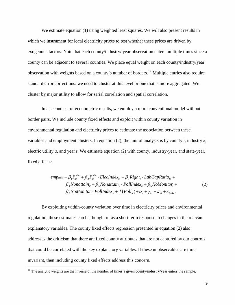
In a second set of econometric results, we employ a more conventional model without

border pairs. We include county fixed effects and exploit within county variation in

environmental regulation and electricity prices to estimate the association between these

variables and employment clusters. In equation (2), the unit of analysis is by county i, industry k,

electric utility u, and year t. We estimate equation (2) with county, industry-year, and state-year,

fixed effects:

.)(7

654

321

iusktstktiitki

ikitit

ktsktelec

utelec

utiuskt

PollfPollIndexNoMonitorNoMonitorPollIndexNonattainNonattain

oLabCapRatiRightElecIndexPPemp

επγαββββ

βββ

+++++⋅++⋅++⋅+⋅+=

(2)

By exploiting within-county variation over time in electricity prices and environmental

regulation, these estimates can be thought of as a short term response to changes in the relevant

explanatory variables. The county fixed effects regression presented in equation (2) also

addresses the criticism that there are fixed county attributes that are not captured by our controls

that could be correlated with the key explanatory variables. If these unobservables are time

invariant, then including county fixed effects address this concern. 14 The analytic weights are the inverse of the number of times a given county/industry/year enters the sample.

10

3. Three Margins Affecting Geographic Concentration of Employment

A key identifying assumption in this paper is that there exists within county border pair

variation in labor regulation intensity, electricity prices, and Clean Air Act intensity that allows

us to observe “exogenous” variation.

3.1. Electricity Prices

Electricity prices vary across electric utility jurisdictions (see Figure 1 for county average

prices in 1998). Adjacent counties can lie within different electric utility jurisdictions. Each of

the approximately 460 U.S. electric utilities charges different electricity prices. In the ideal

research design that relies on county-level employment data, each county would be served by

one utility. In this case, we would have a sharp spatial regression discontinuity at each county

border but this is not the case. Some major counties have multiple utilities. While other utilities

span several counties. If two adjacent counties lie within the same electric utility district, then

there will be no within border pair variation for these counties.15

Most of our border pairs are within the same utility area. However, for those pairs that

cross utilities, the price differences can be significant. The median price differential is about one

cent for border pair counties that lie in different utility areas. For five percent of these counties,

the difference is over nine cents a kWh. For firms in electricity-intensive industries, this

differential represents about seven percent of revenue. This fact highlights that there are

15 Davis et al. (2008) find that, in 2000, about 60 percent of the variation in electricity prices paid by manufacturing plants can be explained by county fixed effects. The remaining differences may be due to multiple utilities serving a county, non-linear pricing where customers are charged both a usage fee and a peak consumption fee, or because of different rates negotiated with the utilities. Davis et al. find evidence of scale economies in delivery that are consistent with observed quantity discounts.

11

significant cost savings for a subset of industries for choosing to locate in the lower electricity

price county within a county-pair.

Most U.S. retail electricity prices are determined through rate hearings where regulated

firms can recover rates through average cost pricing. During the early part of our sample, most

rates were the function of past costs that had little to do with current production costs.16 In

regions that restructured their wholesale electricity markets, retail rates were frozen for an initial

period when utilities were to recover “stranded” assets. Today, the retail prices in these markets

reflect wholesale costs, as passed on to consumers through retail competition.

Our electricity price data are constructed from data available from the Energy

Information Administration (EIA) form 861.17 We determine prices by aggregating revenue from

industrial customers at any utility that serves these customers in a given county and year. We

divide this industrial revenue by the quantity of electricity sold to industrial customers by those

utilities in that year.18 For clustering, we assign the county to one of the 178 major utilities in our

sample.19

16 High capital costs of nuclear plants and Public Utility Regulatory Policy Act (PURPA) contracts from the 1970s and 1980s led to substantial regional variation in retail electricity prices during the 1990s. See Joskow (1989, 2006) for a discussion of retail pricing in the electricity industry.

17 See http://www.eia.doe.gov/cneaf/electricity/page/eia861.html

18 In fact, industrial customers face a non-linear structure that has a per day fixed meter charge, an energy charge per kWh consumed, and an additional demand charge based on peak hourly consumption (kW) during a billing period. In addition, rates may differ by firm size and type. Some large firms face tariffs with a specific tariff that applies to them. Our empirical strategy imposes that firms respond to cross county average price variation when in fact firms will recognize that they face a non-linear pricing schedule.

19 For counties with multiple utilities, the major utility is defined as the utility with the largest total sales across all of its industrial customers.

12

3.2. Labor Regulation

We follow Holmes (1998) and assign each county to whether it is located in a Right-to-

Work state or not. Today, there are 22 states that are Right-to-Work states. A Right-to-Work law

secures the right of employees to decide for themselves whether or not to join or financially

support a union. The set of states includes Alabama, Arizona, Arkansas, Florida, Georgia, Idaho,

Iowa, Kansas, Louisiana, Mississippi, Nebraska, Nevada, North Carolina, North Dakota,

Oklahoma, South Carolina, South Dakota, Tennessee, Texas, Utah, Virginia and Wyoming.

When we restrict our sample to the set of counties that are both in a metropolitan area, we

have relatively few cases in which one county lies in a Right-to-Work state and the other county

lies in non-Right-to-Work State. Two examples of such a “hybrid” metropolitan areas are Kansas

City, Missouri and Washington D.C. Below, we also report results in which we use all U.S.

counties.20

3.3. Environmental Regulation

The Clean Air Act assigns counties to low regulation (Attainment Status) and high

regulation (Nonattainment Status) based on past ambient air pollution readings. Within county

border-pairs, there is variation in environmental regulation both due to cross-sectional

differences (i.e., high regulated counties that are adjacent to less regulated cleaner counties) and

due to changes over time (reclassification of counties from attainment to nonattainment and vice-

20 In metropolitan areas, there are 36 counties that make up 28 different pairs where a state line is crossed. For the full sample, 425 counties abut a state line and make 443 county pairs.

13

versa). In this paper, we focus on ozone as one of the six criteria pollutants. We also estimate

similar models for carbon monoxide and particulate matter.21

We use a continuous measure of ozone pollution intensity.22 We hypothesize that high-

polluting industries—including petroleum and coal products, nonmetallic mineral products, and

paper manufacturing—should be the most responsive to avoiding the nonattainment sides of the

county border pair and in locating in that county within the county border pair that does not

monitor ambient ozone.23 The data indicating a county’s Clean Air Act regulatory status are

from the EPA’s Greenbook.24 Our county/year ambient air pollution data are from the U.S. EPA

AIRS data base. Our regressions include a cubic function of a county’s ambient ozone level.

4. Results

Table 1 reports the summary statistics. The uneven distribution of manufacturing activity

is revealed in the first row. The average county/industry/year observation has 668 jobs but the

median is 111 and the maximum is 158,573. It is relevant to note these summary statistics are

based on all counties located in metropolitan areas and excludes about 75 percent of U.S.

counties. Of this sample, 86 percent have at least one employee in that county, industry, and

year. 21 We estimate equation (1) using two other measures of local environmental regulation intensity: a county’s carbon monoxide (CO) nonattainment status; and a county’s particulate matter (PM) nonattainment status. Our measure of pollution intensity is discussed below. 22 From EPA’s NEI data, we aggregate total tons of emissions by industry, year and pollutant (see ftp://ftp.epa.gov/EmisInventory/2002finalnei/2002_final_v3_2007_summaries/point/allneicap_annual_11302007.zip). For ozone, we aggregate tons of nitrogen oxides and tons of volatile organic compounds. We divide total emissions by the annual value added of each industry (from the NBER productivity data) to construct a pollution intensity index. Finally, we normalize the index to range from zero to one for ease in interpreting coefficients. 23 Ambient air pollution is not monitored in every county. Kahn (1997) documents higher manufacturing growth rates in counties that do not monitor ambient pollution relative to those that do monitor.

24 http://epa.gov/airquality/greenbk/

14

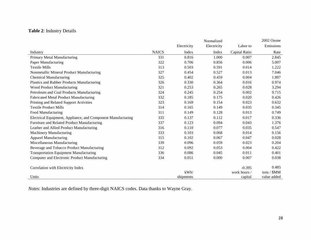
Table 2 reports the names and key statistics for the 21 manufacturing industries that we

study. The rows are sorted from the most energy-intensive industry (Primary Metals) to the least

energy-intensive industry (Computer and Electronic Product Manufacturing). The most energy-

intensive industry uses sixteen times as much electricity per unit of output as the least electricity-

intensive industry. In the right column of Table 2, we report each industry’s labor-to-capital

ratio. Apparel, Leather, Textiles, and Furniture are some of the most labor-intensive industries.

In contrast, the primary metals industry has a tiny labor-to-capital ratio. The cross-industry

correlation between the electricity index and the labor-to-capital ratio equals -0.4.

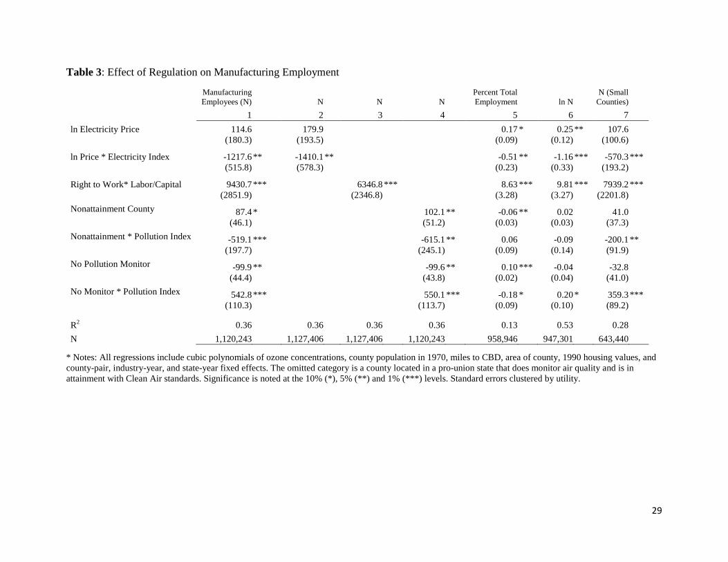
In Table 3, we report our first estimates of equation (1). Recall that each county pair

consists of two metropolitan area counties that are physically adjacent. Controlling for county-

pair fixed effects, industry-year fixed effects, and state-year fixed effects, and a vector of county

attributes (log of land area, log of the distance to the closest metro area’s Central Business

District, the log of the county’s 1970 population, and the log of the 1990 housing values), we

focus on the role of electricity prices and labor and environmental regulation in determining the

geographic location of manufacturing clusters.25 As shown in column (1), we find evidence of a

negative relationship between electricity prices and manufacturing employment activity for all

manufacturing industries whose normalized electricity index is greater than 0.094.26 This

includes all of our industries except electronics (NAICS 334), transportation equipment (NAICS

336) and beverage manufacturing (NAICS 312). We find the largest negative effects of 25 For the first column, when we look at the level of manufacturing employment, we use the level of population in 1970 to be consistent. The results are similar when log historic population is used instead. Recognizing that within a county, such as Los Angeles County, firms may seek out the cheapest utility within the county, we have re-estimated our models using the minimum price in the county and find very similar results.

26 Deschenes (2012) uses a state/year panel approach using a longer time series than we do and does not disaggregate manufacturing industries beyond; “durables” and “non-durables.” Controlling for state and year fixed effects, for “non-durables” he reports a positive correlation of electricity prices and employment based on a specification with state and year fixed effects.

15

electricity prices on primary metals employment. For this industry, we estimate a price elasticity

of -2.17.27

To better understand the magnitude of these effects, assume that a state implemented a

carbon price of $15 per ton of CO2. Given the carbon intensity of producing power in different

regions of the US, this can be mapped into a change in electricity prices (see Kahn and Mansur,

2010). Because of the variation in carbon-intensive electricity markets and energy-intensive

manufacturing across states, our coefficients imply that the employment losses could be much

larger in places like Ohio (21,884 jobs or 3.8% percent) than in California (4,648, or -0.3

percent).28

Controlling for electricity prices, we find that labor-intensive manufacturing clusters on

the Right-to-Work side of the county border pair. For the most labor-intensive industry

(Apparel), the coefficients imply 443 more jobs on the right-to-work side of the border, relative

to an extremely capital-intensive industry like petroleum. This is approximately half of the

average number of workers in a given county/industry/year. It is relevant to contrast this finding

with Holmes’ (1998) work. He finds that the share of total employment that is in manufacturing

is greater by about one third in Right-to-Work states. He did not disaggregate manufacturing into

distinct industries. If the Right-to-Work status simply reflected this overall ideology then we

might not observe that labor-intensive industries are more likely to cluster there. Our finding of a

positive industry-average labor intensity interaction with the state’s labor policies highlights the

importance of allowing for industry disaggregation and is consistent with economic intuition.

27 This is the sum of the coefficient on price and the coefficient on price interacted with the index (which is normalized to range from 0 to 1, where 1 is the most electricity-intensive industry (primary metals)) all divided by the average employment in that industry in our sample: (114.6+(-1217.6)*1)/509=-2.17.

28 See Kahn and Mansur (2010) for a discussion of the assumptions regarding this application.

16

Controlling for electricity prices and labor regulation, we also study the role of

environmental regulation. As expected, we find that employment in high-pollution industries is

lower in high-regulation (nonattainment) counties. We also find that employment is higher for

high-ozone industries in counties that do not monitor ozone.

A distinctive feature of our study is that we simultaneously study the marginal effects of

energy prices, labor regulation, and environmental regulation in one unified framework. In Table

3’s columns (2-4), we present our estimates for what we would find if we studied these variables

individually. In column (2), we find that the electricity price interaction grows more negative by

16% and the labor intensity interaction shrinks by roughly 33% and the environmental regulation

interaction grows more negative by roughly 19%.

The results in column (5) of Table 3 switch the dependent variable to the ratio of a

county/year’s jobs in a given industry divided by total county employment. This was Holmes’

(1998) dependent variable. This measure better captures the composition of jobs within a county.

The electricity price and labor regulation results are similar to the results in column (1) but we

find no evidence of the importance of environmental regulation. For the primary metals industry,

we find that a ten percent increase in electricity prices is associated with a 0.034 percentage point

reduction in the share of workers in the county who works in this industry.

In Table 3’s column (6), we use the log of the county/industry/year’s employment and

thus lose the observations for which there are zero jobs. The electricity price and labor policy

results are qualitatively quite similar to those reported in equation (1). Based on this

specification, we estimate an employment electricity price elasticity of -.91 for the primary

metals industry. However, the coefficients on environmental regulation are noisy. Overall, we

17

find mixed evidence that environmental regulation affects pollution-intensive manufacturing jobs

more than others.

Following Holmes (1998), the last column of Table 3 includes just small counties.

Namely, the sample consists of paired counties whose centroids are within 30 miles of each

other. Small counties are more likely to have similar unobserved shocks. Of course, smaller

counties are likely to be in more densely populated areas as well, so we are exploring a different

subset of the population. We find that the main results are qualitatively robust, with similar signs

and significance, as our main findings. However, the policy effects are attenuated suggesting that

there is heterogeneity in the employment effects between large and small counties. Appendix

Table A2 explores a range of distances.

Given the estimates in column (1) of Table 3, we can now compare the relative

sensitivities of a given industry to energy prices, labor policy, and environmental policies. For an

industry like petroleum—which is energy intensive, capital intensive, and a high-ozone

polluter—banning Right-to-Work laws would have the same effect on employment as an eight

percent increase in electricity prices. In contrast, if a petroleum manufacturer’s county falls into

nonattainment with environmental regulations, this is akin to tripling electricity prices. Other

industries that are not energy or pollution intensive are not as negatively affected by either higher

energy prices or pollution regulation. For example, for apparel manufacturing, repealing a right-

to-work law is akin to a fourfold increase in electricity prices.

In Table 4, we modify equation (1) by estimating separate coefficients on electricity

prices for each manufacturing industry. In other words, we relax the index restriction on

electricity prices that was imposed on the results reported in Table 3. We also estimate equation

18

(1) separately for fifteen major non-manufacturing industries.29 The results reported in Table 4

focus on the role of energy prices. We do not include labor or environmental regulations in these

regressions. We report results for three dependent variables: the employment level, the industry’s

share of county employment and log employment. For ten manufacturing industries, we find

negatively statistically significant correlations (at the five percent level) for the level of

employment and electricity prices. For log employment, we find a negative correlation for seven

of the industries. In the case of the share regressions, we find fewer negative correlations and

actually find positive correlations for industries such as Textile Products (NAICS 314),

Computers (NAICS 334) and Miscellaneous (NAICS 339). These two industries each have a

very low energy intensity index. Finally, we note that Tables 3 and 4 imply similar employee-

weighted average elasticities across industries for each specification.30

The bottom panel of Table 4 reports similar regressions for non-manufacturing industries.

Many of these industries employ millions of people and have experienced sharp employment

growth between 1998 and 2009. Employment in expanding industries such as Credit

Intermediation (NAICS 522), Professional, Scientific and Technical Services (NAICS 541), and

Management of Companies and Enterprises (NAICS 551) is responsive to electricity prices with

elasticities of approximately -.15. However, for most non-manufacturing industries, we find that

energy prices are not an important correlate of geographical concentration. An examination of

29 We choose the 15 industries with the most employees in 1998. Wholesale electronic markets (NAICS 425) had the ninth most jobs in 1998 but the NAICS 2002 reclassifications made it difficult to track this industry. Instead, we added the 16th most common job in 1998, Motor Vehicle and Parts Dealers (NAICS 441). Note that the border-pair and state-year fixed effects differ by non-manufacturing industry but are pooled for manufacturing industries.

30 For the linear specification, the implied elasticity is -.30 in Table 3 and -.41 in Table 4. For the log specification, they are .00 and -.10, respectively. Note that the log specification is conditional on any employment in the county/industry/year and therefore need not be the same as the linear model.

19

BEA electricity cost shares indicates that there is not a cross-industry negative correlation

between electricity prices and electricity cost shares for non-manufacturing industries.31

Additional Empirical Tests

In this section, we report additional regression results to test how our core results are

affected by changing the sample, the sample years, including additional control variables and

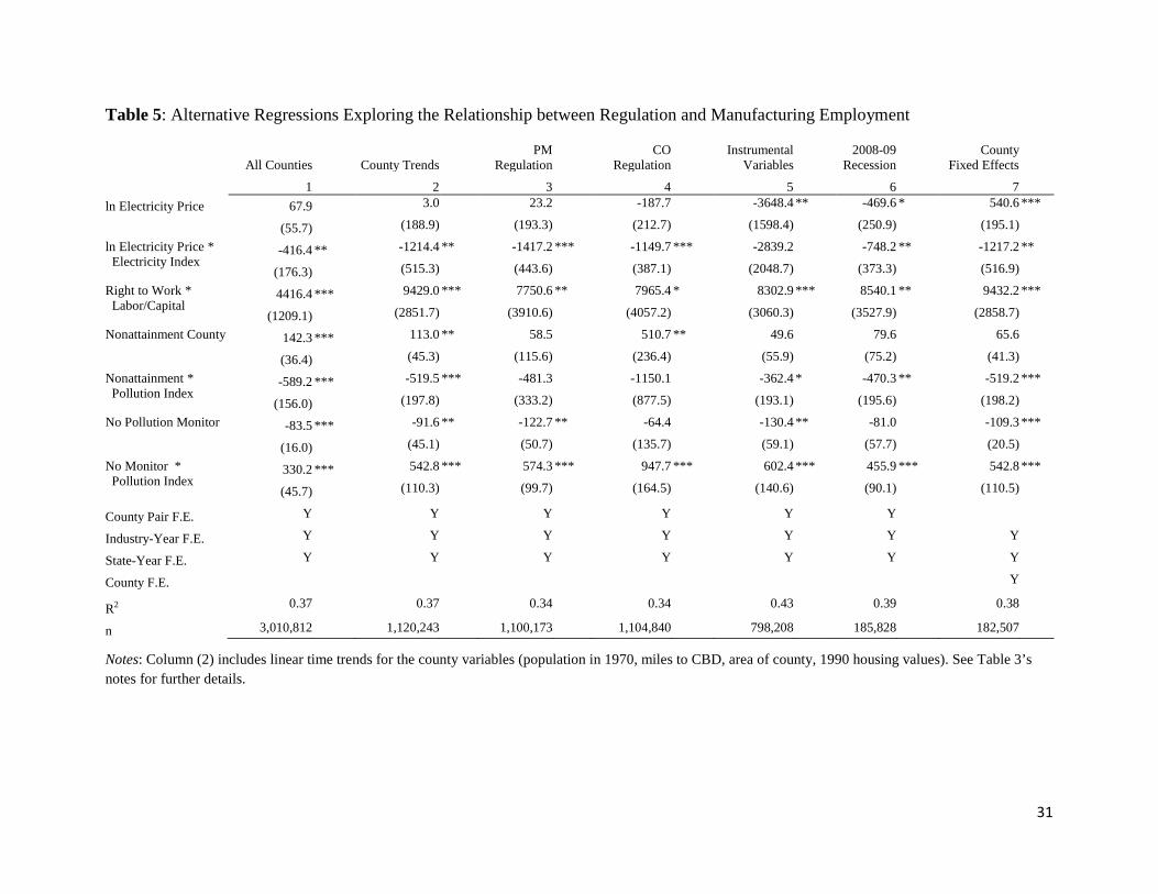
using different regulatory intensity measures. In Table 5’s column (1), we report our results

using all of the counties in the continental United States. Relative to the metro sample, the results

for the full county sample yield the same coefficient signs but the absolute value of the

coefficients for electricity prices and labor regulation shrinks by more than 50 percent. The

coefficients on environmental regulation indicators shrink but by a much smaller percentage. In

Table 5’s column (2), we include linear time trends for each control variable such as population

and home values to control for the possibility that counties differ with respect to their growth

trajectory. The results are robust for controlling for these trends. Column’s (3) and (4) use

particulate matter and carbon monoxide pollution in place of the ozone for attainment status,

monitoring status, high polluter industries, and concentration ratios. We find similar coefficients

as in our main results but larger standard errors.32

We recognize that there are cases in which a county’s average electricity price could be

correlated with the error term. A demand side explanation argues that a boom in local

31 We use Bureau of Economic Analysis (BEA) input-output data to construct electricity cost shares. See http://www.bea.gov/industry/io_benchmark.htm. Using data for 2002, we define the cost share as the ratio of an industry’s dollars spent on electric power (NAICS 2211) over its total industry output.

32 These results are not surprising given the few number of counties in nonattainment with these pollutants.

20

employment will result in an increase in the utility’s demand. This requires more expensive

power plants to operate, and electricity prices will increase. Second, industrial firms have some

bargaining power in negotiating rates with the electric utility. Third, imprecise measurement of a

firm’s electricity price: measurement error leads to an attenuation bias of OLS estimates. To

address these concerns, we present instrumental variables results in Table 5’s column (5). We

construct instruments using the product of the local utility’s capacity shares of coal, oil and gas-

fired power plants and the respective annual average fuel price.33 The sample size declines

because we are missing fuel shares for some utilities. The F-Statistic for the first stage equals

1139. The key finding to emerge in this instrumental variables case is that all industries (even

those with the lowest energy intensity) now have a negative employment elasticity with respect

to energy prices and the effect is much larger. The other coefficients on labor and environmental

regulation are consistent with our core hypotheses.

The recent deep recession has highlighted the importance of U.S manufacturing to our

economy. During a recession, few firms are creating jobs but industries and locations may differ

with respect to the rate that they are shedding jobs. In Table 5’s column (6), we re-estimate

equation (1) using just two years of the data; 2008 and 2009 to see how our key explanatory

variables affect employment during a major recession. The results are qualitatively similar to the

full sample results reported in Table 3’s column (1) but the negative effect of electricity prices on

33 The shares data are from the EIA form 860 data for 1995. The fuel prices are from the EIA: coal prices are quantity-weighted annual averages from EIA form 423; oil prices are the spot WTI; and natural gas prices are the annual Henry Hub contract 1 prices.

21

employment now holds for all industries. For the most electricity intensive industry, the implied

elasticity is -1.69.34

An alternative strategy for studying the role of regulations and electricity prices on

employment is to estimate equation (2) and include county fixed effects. In this case, the key

interaction effects are identified from within county yearly variation in electricity prices, and the

county’s regulatory intensity and national changes in the industry’s annual pollution intensity,

labor intensity and electricity intensity. As shown in column (7), the results are remarkably

similar to our results reported in Table 3’s column (1) when we include border-pair fixed

effects.35

Regulation’s Impact on Industrial Organization

The County Business Patterns data provides information for each county/industry/year on its

employment count and establishment count. In Table 6, we use these two pieces of information

and in addition we calculate the average employment count per establishment. We report

regression estimates of equation (1) using each of these as the dependent variable. Table 6’s

column (1) is identical to Table 3’s column (1). In column (2), we report the establishment count

34 We have also estimated this regression using data from 2007 to 2009 and find quite similar results.

35 Incumbent firms are likely to face migration costs to relocate. If large capital costs are sunk, firms may delay relocating until their existing production facility depreciates or there are large differences in operating costs across geographic locations. One example is the Ocean Spray Corporation which plans to close its 250-worker cranberry concentrate processing plant in Bordentown, New Jersey in September 2013, and move it to Lehigh or Northampton counties in Pennsylvania. The closing facility is old and high cost. The company has claimed that it is attracted to the new Pennsylvania location because of lower power, water and trucking costs (http://www.philly.com/philly/blogs/inq-phillydeals/South-Jersey-plant-to-close-250-jobs-moved-report.html).

22

regression. We find that the count of establishments responds to both electricity prices and to

environmental regulation. Establishments that are energy intensive avoid the high electricity

price counties. We cannot reject the hypothesis that there is no correlation between labor

regulation and the establishment count. In column (3), we switch the dependent variable to the

log of the establishment count. In this case, we find that there are more labor-intensive

establishments clustering on the Right-to-Work side of the border. We continue to find evidence

that electricity prices and ozone regulation are determinants of establishments. In columns (4)

and (5) of Table 6, we report regression results for two measures of facility size: the ratio of

workers per establishment, and its log. Bigger firms avoid the high electricity price county.

Surprisingly, we find no statistically significant correlation between a county’s Right-to-Work

status and the size of facilities even for labor-intensive industries. Based on the results in column

(4), smaller firms in high ozone industries are clustering in counties that do not monitor ozone.

5. Conclusion

The basic logic of cost minimization offers strong predictions concerning where different

manufacturing industries will cluster across U.S. counties as a function of regulatory policies and

input prices. Using a unified framework that exploits within county-pair variation in locational

attributes, we have documented that labor-intensive industries locate in anti-union areas, energy-

intensive industries locate in low electricity price counties and high polluting industries seek out

low regulation areas. Based on our findings, we conclude that energy prices are a significant

determinant of locational choice for a handful of manufacturing industries such as primary

metals. For the typical manufacturing industry, the electricity price effects are modest.

23

Our analysis highlights the importance of studying the marginal effects of energy

regulation, labor regulation and environmental regulation at the same time. Republican “Red

States” tend to have low electricity prices, and be Right to Work states while Democratic “Blue

States” tend to have higher electricity prices and support union rights. Both types of states are

roughly likely to have counties assigned to pollution non-attainment status. This paper’s

empirical strategy has allowed us to estimate the marginal and total effects of this bundle of

policies.

We summarize our results in Table 7. Notably, the most intensive industries in electricity,

labor and pollution are much more sensitive to their respective policies. For example, the

electricity price elasticity is over two for primary metals but is inelastic and only weakly

significant for the industry of the average worker in our sample. Labor and environmental

policies have huge effects on their most intensive industries, apparel and coal/petroleum

respectively, but hardly matter for the average industry.

We anticipate future research will access census micro data for manufacturing plants.

Such data would allow researchers to make more progress on the likely mechanisms underlying

the aggregate effects we report. At the extensive margin, do incumbent firms exit areas where

environmental regulations tighten and electricity prices increase? Or, do existing firms respond

by reducing their output and hence their consumption of inputs? Anticipating the persistence of

these policies do firms make investments to alter their use of the relatively more costly input?

24

References

Becker, Randy and Vernon Henderson. 2000. “Effects of Air Quality Regulations on Polluting Industries,” Journal of Political Economy, 108(2): 379–421.

Bernard, Andrew B., J. Bradford Jensen, and Peter K. Schott. 2006. “Survival of the Best Fit: Exposure to Low-Wage Countries and the (Uneven) Growth of U.S. Manufacturing Plants,” Journal of International Economics, 68(1): 219-237.

Carlton, Dennis. 1983. “The Location and Employment Choices of New Firms: An Econometric Model with Discrete and Continuous Endogenous Variables,” Review of Economics and Statistics, 65(3): 440-449.

Chirinko, Robert S. and Daniel J. Wilson. 2008. “State Investment Tax Incentives: A Zero-Sum Game?” Journal of Public Economics, 92(12): 2362-2384.

Davis, Steven J., R. Jason Faberman, John Haltiwanger. 2006. “The Flow Approach to Labor Markets: New Data Sources and Micro–Macro Links,” Journal of Economic Perspectives, 20(3): 3-26.

Davis, Steven, Cheryl Grim, John Haltiwanger, and Mary Streitwieser. 2008. “Electricity Pricing to U.S. Manufacturing Plants, 1963–2000,” National Bureau of Economic Research Working Paper No. 13778.

Deschenes, Olivier. 2012. “Climate Policy and Labor Markets,” in The Design and Implementation of U.S Climate Policy, Don Fullerton and Catherine Wolfram, ed. University of Chicago Press.

Dube, Arindrajit, T. William Lester, and Michael Reich. 2010. “Minimum Wage Effects Across State Borders: Estimates Using Contiguous Counties,” Review of Economics and Statistics, 92(4): 945-964.

Dumais, Guy, Glen Ellison, and Edward Glaeser. 2002. “Geographic Concentration as a Dynamic Process,” Review of Economics and Statistics, 84(2): 193-204.

Ellison, Glen and Edward Glaeser. 1999. “The Geographic Concentration of Industry: Does Natural Advantage Explain Agglomeration?” American Economic Review Papers and Proceedings, 89(2): 311-317.

Greenstone, Michael. 2002. “The Impacts of Environmental Regulation on Industrial Activity,” Journal of Political Economy, 110(6): 1175–1219.

Greenstone, Michael, Richard Hornbeck, and Enrico Moretti. 2010. “Identifying Agglomeration Spillovers: Evidence from Million-Dollar Plants.” Journal of Political Economy, 118(3): 536-598.

Holmes, Thomas. 1998. “The Effect of State Policies on the Location of Manufacturing: Evidence from State Borders,” Journal of Political Economy, 106(4): 667–705.

Isserman, Andrew and James Westervelt. 2006. “1.5 Million Missing Numbers: Overcoming Employment Suppression in the County Business Patterns Data,” International Regional Science Review, 29(3): 311-335.

25

Joskow, Paul L. 1989. “Regulatory Failure, Regulatory Reform and Structural Change in the Electric Power Industry,” Brookings Papers on Economic Activity: Microeconomics, 125-199.

Joskow, Paul L. 2006. “Markets for Power in the U.S.: An Interim Assessment,” The Energy Journal, 27(1): 1-36.

Kahn, Matthew E. 1997. “Particulate Pollution Trends in the United States,” Regional Science and Urban Economics, 27(1): 87-107.

Kahn, Matthew E. and Erin T. Mansur. 2010. “How Do Energy Prices, and Labor and Environmental Regulations Affect Local Manufacturing Employment Dynamics? A Regression Discontinuity Approach,” NBER Working Paper 16538.

Killian, Lutz. 2008. “The Economic Effects of Energy Price Shocks,” Journal of Economic Literature, 46(4): 871‐909.

Linn, Joshua. 2009. “Why Do Energy Prices Matter? The Role of Interindustry Linkages In U.S. Manufacturing,” Economic Inquiry,47(3): 549-567.

Neal, Derek, 1995. “Industry-Specific Human Capital: Evidence from Displaced Workers,” Journal of Labor Economics, 13(4): 653-677.

26

Figure 1: Industrial Electricity Prices in 1998 ($/kWh)

27

Table 1: Summary Statistics

1st

3rd

Variable Units Obs Mean Std. Dev. Min Quartile Median Quartile Max

Mnfct. Employees workers 157,459 668 2,373 0 10 111 515 158,573

% Total Emp. % 157,459 0.7% 1.8% 0.0% 0.0% 0.2% 0.7% 56.4%

ln(Employment)

135,531 4.97 2.05 0.00 3.54 5.19 6.48 11.97

Any Manufacturing 0/1 157,459 0.86 0.35 0.00 1.00 1.00 1.00 1.00

Suppressed Data 0/1 157,459 0.43 0.50 0.00 0.00 0.00 1.00 1.00

Electricity Price $/kWh 157,459 $0.065 $0.024 $0.000 $0.050 $0.057 $0.069 $0.523

Electricity Index kWh/shipments 157,459 0.33 0.23 0.00 0.16 0.22 0.44 1.00

Right to Work Laws 0/1 157,459 0.44 0.50 0.00 0.00 0.00 1.00 1.00

Labor/Capital Ratio work hours/

capital 157,459 0.018 0.013 0.001 0.008 0.015 0.024 0.076

Ozone Emis. Rate tons/ $MM value added 157,459 1.79 2.55 0.03 0.34 0.63 1.90 9.71

Ozone Nonattain. 0/1 157,459 0.34 0.47 0.00 0.00 0.00 1.00 1.00

PM Nonattainment 0/1 157,459 0.11 0.32 0.00 0.00 0.00 0.00 1.00

CO Nonattainment 0/1 157,459 0.04 0.19 0.00 0.00 0.00 0.00 1.00

Notes: An observation is by county, year, and 3-digit NAICS industry code. Index is normalized to range from zero to one.

28

Table 2: Industry Details

Normalized

2002 Ozone

Electricity Electricity Labor to Emissions

Industry NAICS Index Index Capital Ratio Rate Primary Metal Manufacturing 331 0.816 1.000 0.007 2.845 Paper Manufacturing 322 0.706 0.856 0.006 5.007 Textile Mills 313 0.503 0.591 0.014 1.222 Nonmetallic Mineral Product Manufacturing 327 0.454 0.527 0.013 7.046 Chemical Manufacturing 325 0.402 0.459 0.004 1.897 Plastics and Rubber Products Manufacturing 326 0.330 0.364 0.016 0.974 Wood Product Manufacturing 321 0.253 0.265 0.028 3.294 Petroleum and Coal Products Manufacturing 324 0.245 0.254 0.002 9.715 Fabricated Metal Product Manufacturing 332 0.185 0.175 0.020 0.426 Printing and Related Support Activities 323 0.169 0.154 0.023 0.632 Textile Product Mills 314 0.165 0.149 0.035 0.345 Food Manufacturing 311 0.149 0.128 0.013 0.749 Electrical Equipment, Appliance, and Component Manufacturing 335 0.137 0.112 0.017 0.336 Furniture and Related Product Manufacturing 337 0.123 0.094 0.043 1.376 Leather and Allied Product Manufacturing 316 0.110 0.077 0.035 0.547 Machinery Manufacturing 333 0.103 0.068 0.014 0.156 Apparel Manufacturing 315 0.102 0.067 0.047 0.028 Miscellaneous Manufacturing 339 0.096 0.059 0.023 0.204 Beverage and Tobacco Product Manufacturing 312 0.092 0.053 0.004 0.422 Transportation Equipment Manufacturing 336 0.086 0.045 0.011 0.401 Computer and Electronic Product Manufacturing 334 0.051 0.000 0.007 0.038

Correlation with Electricity Index

-0.395 0.485

Units kWh/

shipments work hours /

capital tons / $MM value added

Notes: Industries are defined by three-digit NAICS codes. Data thanks to Wayne Gray.

29

Table 3: Effect of Regulation on Manufacturing Employment

Manufacturing Employees (N)

N N N

Percent Total Employment ln N

N (Small Counties)

1 2 3 4 5 6 7

ln Electricity Price 114.6

179.9 0.17 * 0.25 ** 107.6 (180.3)

(193.5) (0.09) (0.12) (100.6)

ln Price * Electricity Index -1217.6 ** -1410.1 ** -0.51 ** -1.16 *** -570.3 *** (515.8)

(578.3) (0.23) (0.33) (193.2)

Right to Work* Labor/Capital 9430.7 *** 6346.8 *** 8.63 *** 9.81 *** 7939.2 *** (2851.9)

(2346.8) (3.28) (3.27) (2201.8)

Nonattainment County 87.4 * 102.1 ** -0.06 ** 0.02 41.0 (46.1)

(51.2) (0.03) (0.03) (37.3)

Nonattainment * Pollution Index -519.1 *** -615.1 ** 0.06 -0.09 -200.1 ** (197.7)

(245.1) (0.09) (0.14) (91.9)

No Pollution Monitor -99.9 ** -99.6 ** 0.10 *** -0.04 -32.8 (44.4)

(43.8) (0.02) (0.04) (41.0)

No Monitor * Pollution Index 542.8 *** 550.1 *** -0.18 * 0.20 * 359.3 *** (110.3)

(113.7) (0.09) (0.10) (89.2)

R2 0.36

0.36 0.36 0.36 0.13 0.53 0.28 N 1,120,243 1,127,406 1,127,406 1,120,243 958,946 947,301 643,440

* Notes: All regressions include cubic polynomials of ozone concentrations, county population in 1970, miles to CBD, area of county, 1990 housing values, and county-pair, industry-year, and state-year fixed effects. The omitted category is a county located in a pro-union state that does monitor air quality and is in attainment with Clean Air standards. Significance is noted at the 10% (*), 5% (**) and 1% (***) levels. Standard errors clustered by utility.

30

Table 4: Employment Regressions by Industry

Employees in Industry BEA Elect.

ln N

Employees

NAICS 1998 (1000s) Growth Cost Share Manufacturing Industries Coef. S.E. Coef. S.E.

311 1,464 -.004% 1.17% Food 0.03 (0.24) 239 (311)

312 173 -10% 0.79% Beverage & Tobacco Product 0.02 (0.41) -890 (396) **

313 385 -51% 2.40% Textile Mills -0.31 (0.58) -970 (344) ***

314 217 -28% 0.77% Textile Product Mills 0.17 (0.16) -905 (312) ***

315 671 -68% 0.54% Apparel 0.25 (0.32) 227 (434)

316 79 -53% 0.66% Leather & Allied Product -0.10 (0.27) -1026 (380) ***

321 580 -1% 1.35% Wood Product -0.59 (0.23) ** -1008 (329) ***

322 568 -22% 3.34% Paper -0.47 (0.22) ** -728 (303) **

323 845 -24% 0.99% Printing & Related Activities 0.27 (0.11) ** -60 (119)

324 111 -7% 0.78% Petroleum & Coal Products -0.59 (0.25) ** -1007 (371) ***

325 901 -11% 3.49% Chemical 0.08 (0.19) 143 (317)

326 1030 -13% 1.82% Plastics & Rubber Products -0.24 (0.15) -240 (194)

327 508 -5% 2.20% Nonmetallic Mineral Product -0.33 (0.17) ** -723 (287) **

331 615 -27% 3.40% Primary Metal -1.17 (0.26) *** -1053 (331) ***

332 1,816 -14% 1.42% Fabricated Metal Product -0.18 (0.14) 979 (555) *

333 1,444 -22% 0.47% Machinery -0.31 (0.18) * -211 (260)

334 1,681 -37% 0.27% Computer & Electronic Product 0.67 (0.26) ** 2185 (910) **

335 602 -30% 0.66% Electrical Equipment, Appliance 0.11 (0.20) -574 (256) **

336 1,911 -15% 0.21% Transportation Equipment -0.80 (0.28) *** -243 (578)

337 604 -10% 0.70% Furniture & Related Product -0.11 (0.14) -584 (155) ***

339 737 -7% 0.49% Miscellaneous 0.71 (0.12) *** 574 (194) ***

Other Industries

238 8,926 26% 1.28% Specialty Trade Contractors 0.10 (0.06) * -825 (576)

441 1,757 11% 1.28% Motor Vehicle & Parts Dealers -0.06 (0.06) -797 (315) **

445 2,944 -1% 1.28% Food & Beverage Stores 0.03 (0.12) -786 (412) *

452 4,263 -34% 1.28% General Merchandise Stores -0.07 (0.06) -549 (288) *

522 2,688 22% 0.10% Credit Intermediation & Related -0.15 (0.08) * -277 (350)

524 2,312 3% 0.11% Insurance Carriers & Related -0.22 (0.12) * -340 (389)

541 6,052 33% 0.19% Professional, Scientific & Techn. -0.18 (0.09) * -4099 (1717) **

551 2,704 8% 0.63% Management of Companies -0.15 (0.13) -1514 (540) ***

561 8,366 27% 0.28% Administrative & Support -0.07 (0.11) -3151 (1245) **

611 2,324 28% 2.18% Educational Services 0.02 (0.11) -81 (605)

621 4,482 27% 0.35% Ambulatory Health Care 0.07 (0.05) -14 (528)

622 5,011 7% 1.13% Hospitals -0.13 (0.11) 463 (477)

623 2,511 19% 1.38% Nursing & Residential Care 0.14 (0.05) *** 107 (191)

722 7,758 22% 1.96% Food Services & Drinking Places 0.00 (0.04) -2854 (1218) **

813 2,488 12% 0.20% Religious, Grantmaking, Civic -0.04 (0.04) 14 (187) * Notes: For manufacturing industries, we modify equation (1) so each industry has a separate price coefficient. For non-manufacturing industries, we estimate equation (1) separately for each industry. Industry growth is from 1998 to 2006. See Table 3’s notes for further details.

31

Table 5: Alternative Regressions Exploring the Relationship between Regulation and Manufacturing Employment

All Counties

County Trends

PM Regulation

CO Regulation

Instrumental Variables

2008-09 Recession

County Fixed Effects

1 2 3 4 5 6 7

ln Electricity Price 67.9 3.0 23.2 -187.7 -3648.4 ** -469.6 * 540.6 ***

(55.7) (188.9) (193.3) (212.7) (1598.4) (250.9) (195.1)

ln Electricity Price * Electricity Index

-416.4 ** -1214.4 ** -1417.2 *** -1149.7 *** -2839.2 -748.2 ** -1217.2 **

(176.3) (515.3) (443.6) (387.1) (2048.7) (373.3) (516.9)

Right to Work * Labor/Capital

4416.4 *** 9429.0 *** 7750.6 ** 7965.4 * 8302.9 *** 8540.1 ** 9432.2 ***

(1209.1) (2851.7) (3910.6) (4057.2) (3060.3) (3527.9) (2858.7)

Nonattainment County 142.3 *** 113.0 ** 58.5 510.7 ** 49.6 79.6 65.6

(36.4) (45.3) (115.6) (236.4) (55.9) (75.2) (41.3)

Nonattainment * Pollution Index

-589.2 *** -519.5 *** -481.3 -1150.1 -362.4 * -470.3 ** -519.2 ***

(156.0) (197.8) (333.2) (877.5) (193.1) (195.6) (198.2)

No Pollution Monitor -83.5 *** -91.6 ** -122.7 ** -64.4 -130.4 ** -81.0 -109.3 ***

(16.0) (45.1) (50.7) (135.7) (59.1) (57.7) (20.5)

No Monitor * Pollution Index

330.2 *** 542.8 *** 574.3 *** 947.7 *** 602.4 *** 455.9 *** 542.8 ***

(45.7) (110.3) (99.7) (164.5) (140.6) (90.1) (110.5)

County Pair F.E. Y Y Y Y Y Y

Industry-Year F.E. Y Y Y Y Y Y Y

State-Year F.E. Y Y Y Y Y Y Y

County F.E. Y

R2 0.37 0.37 0.34 0.34 0.43 0.39 0.38

n 3,010,812 1,120,243 1,100,173 1,104,840 798,208 185,828 182,507 Notes: Column (2) includes linear time trends for the county variables (population in 1970, miles to CBD, area of county, 1990 housing values). See Table 3’s notes for further details.

32

Table 6: Regulation and Establishment Characteristics

Notes: See Table 3’s notes for details.

Employees Establishments Log

Establishment Workers per

Establishment Log (Workers per

Establishment) 1 2 3 4 5 ln Electricity Price 114.6 6.3 ** 0.12 * 10.9 ** 0.12 ** (180.3) (2.8) (0.07) (4.4) (0.06)

ln Price * Electricity Index

-1217.6 ** -38.1 ** -0.57 *** -42.3 *** -0.59 *** (515.8) (14.8) (0.20) (12.0) (0.14)

Right to Work* Labor/Capital

9430.7 *** -14.1 7.46 *** -117.0 2.34 (2851.9) (78.4) (1.82) (115.6) (1.73)

Nonattainment County 87.4 * 3.0 *** 0.05 *** -4.3 *** -0.03 (46.1) (1.1) (0.02) (1.6) (0.02)

Nonattainment * Pollution Index

-519.1 *** -17.9 *** -0.17 ** 12.3 * 0.08 (197.7) (5.8) (0.08) (6.4) (0.10)

No Pollution Monitor -99.9 ** -1.6 -0.05 * 4.4 *** 0.01 (44.4) (1.0) (0.03) (1.5) (0.02)

No Monitor * Pollution Index

542.8 *** 13.5 *** 0.25 *** -11.2 * -0.06 (110.3) (2.9) (0.06) (6.4) (0.07)

R2 0.36 0.44 0.77 0.14 0.28

n 1,120,243 1,120,243 947,301 947,290 947,290

33

Table 7: Summary Table of Main Results Regulation or Price Least Intensive Average Most Intensive

Electricity Computer Manuf. Primary Metals Ave N 1565 696 509 Norm. Elec. Index 0.00 0.28 1.00 Electricity Price Elasticity 0.073 -0.204 * -2.166 ***

(0.115) (0.120) (0.815)

Labor Petroleum and Coal Apparel Ave N 121 696 331 L/K Ratio 0.002 0.016 0.047 Right-to-Work Percentage 11.7% *** 21.0% *** 135.2% ***

(0.035) (0.064) (0.409)

Pollution Apparel Petroleum and Coal Ave N 331 696 121 Norm. Ozone Index 0.00 0.11 1.00 Ozone Nonatt. Percentage 26.4% * 4.1% -356.8% ***

(0.139) (0.045) (1.351)

Ozone No Monitor Percentage -30.2% ** -5.5% 366.1% ***

(0.134) (0.056) (0.780)

Notes: See Table 3’s notes for details. Average is a worker-weighted average of county-industry-year observations in our sample.