how did the financial crisis affect daily stock returns?

THE JOURNAL OF INVESTING 65FALL 2014

How Did the Financial Crisis Affect Daily Stock Returns?MO CHAUDHURY

MO CHAUDHURY

is a professor of practice in finance at the Desautels Faculty of Management at McGill University in Montreal, QC, [email protected]

The headline of the 2007–2008 f inancial crisis is that the stock market, especially the f inancial stocks, plummeted during the

crisis. Surely, this is so on a cumulative basis, but for numerous users and applications, it is the various features of the short interval, most popularly daily, stock returns that are of utmost importance.

Surprisingly, we found very little pub-licly available research on the behavior of daily stock returns during crises. Kho and Stulz [1999] found that the Asian bank share-holders suffered drastically while the Western banks performed better than their national markets during the 1997–1998 Asian crisis. Bartram and Bodnar [2009] studied the nature of cumulative value destruction and correla-tion in world equity markets and sectors in relation to key events during the 2007–2008 crisis, especially in the fall of 2008. But they do not examine the properties of daily stock price change nor do they study individual stocks. Dwyer and Tkac [2009] provided primarily a conceptual understanding of the effects of the f inancial crisis in the f ixed-income markets. Lioui [2009] and Marsh and Niemer [2008] studied the consequences of banning short sales during the financial crisis, while Schwert [2011] focused solely on volatility.

This article attempts to close an apparent gap in the literature concerning the

effect of the crisis on a number of promi-nent features/properties of daily stock price changes, namely, central moments of the unconditional distribution other than vola-tility (mean, skewness, and kurtosis), cor-relation with other stocks, the market or beta risk and its relative importance, per-formance on a market-risk-adjusted basis ( Jensen’s alpha), dynamics of conditional variance (persistence, leverage, volatility risk premium) and tail risk (value at risk or VaR). These properties of daily returns are the most pertinent in a wide variety of appli-cations, such as cost of equity estimation, asset allocation, active trading strategies and portfolio management, valuation of deriva-tives, setting of bid–ask spreads and margin requirements, hedging, and measurement and management of market risk exposure, the associated regulatory and economic cap-ital and/or collateral, and so on.

The contribution of this article to the literature lies in examining the effect of the unprecedented financial crisis on the impor-tant properties of daily returns for 31 major non-financial and financial stocks in the U.S., some equally weighted portfolios of these stocks, and the S&P 500 Index. As expected, we find that the unconditional mean daily returns fell significantly to negative levels and the unconditional volatility exploded during the crisis. But contrary to popular belief, the correlation between the financial and non-

The

Jou

rnal

of

Inve

stin

g 20

14.2

3.3:

65-8

4. D

ownl

oade

d fr

om w

ww

.iijo

urna

ls.c

om b

y M

o C

haud

hury

on

09/0

3/14

.It

is il

lega

l to

mak

e un

auth

oriz

ed c

opie

s of

this

art

icle

, for

war

d to

an

unau

thor

ized

use

r or

to p

ost e

lect

roni

cally

with

out P

ublis

her

perm

issi

on.

66 HOW DID THE FINANCIAL CRISIS AFFECT DAILY STOCK RETURNS? FALL 2014

financial stocks actually declined over the course of the crisis. The beta of the financial stocks rose sharply, thus elevating their cost of equity capital substantially. But, in a puzzling manner, they still beat the market with a stunning level (+0.2072) of Jensen’s alpha in the later stage of the crisis as the market rewarded the financials despite plunging profits and heightened risk. Interest-ingly, the relative importance of the market risk actually dropped for the financial stocks as the sector-specific developments for the sector increased their non-market risk.

Using the GARCH (1,1) in mean and EGARCH (1,1) in mean models,1 we observe a significant increase in variance persistence for the S&P 500 and the financial stocks as the crisis unfolded. For their part, the non-financial stocks show a mixed pattern. The leverage effect in the later stage of the crisis is generally stronger compared with the pre-crisis period, but the increase in the leverage effect was not that large or pervasive across stocks. This casts doubt on whether there is a strong systematic or market-based leverage factor in the conditional variance dynamics of stocks.

We find a weaker negative skew to positive skew in the unconditional physical distribution of the indi-

vidual stocks and portfolios during the crisis period. The kurtosis evidence is mixed at the individual stock level, while there was a large drop in the unconditional kurtosis of the S&P 500. Lastly, as expected, the tail risk (99% VaR) of the stock portfolios rose sharply during the crisis. But importantly, this seems driven by the rise in the unconditional volatility and not by departure from normality. Thus, it is not the VaR measure of tail risk or the normality assumption, it is rather the failure to forecast the unprecedented level of unconditional volatility that led to the widespread capital inadequacy and stress among financial institutions.

THE FINANCIAL CRISIS

Gorton [2008]; Longstaff [2008]; and Lo [2012], among others, provide extensive information and anal-ysis of the financial crisis. In the first quarter of 2007, the Case-Shiller Price Index recorded the first year-over-year housing price decline on a national basis since 1991. The stock market remained stunningly complacent, however, until May 2008, as can be seen in Exhibit 1, which plots the daily closing level of the Dow Jones Industrial Average (DJIA), the S&P 500 Index, and the

E X H I B I T 1Stock Market Behavior: Daily Closing Levels, January 1, 2007–December 31, 2008

Source: Yahoo Finance.

The

Jou

rnal

of

Inve

stin

g 20

14.2

3.3:

65-8

4. D

ownl

oade

d fr

om w

ww

.iijo

urna

ls.c

om b

y M

o C

haud

hury

on

09/0

3/14

.It

is il

lega

l to

mak

e un

auth

oriz

ed c

opie

s of

this

art

icle

, for

war

d to

an

unau

thor

ized

use

r or

to p

ost e

lect

roni

cally

with

out P

ublis

her

perm

issi

on.


closing price of the f inancial sector exchange-traded fund (XLF). During the short span of May 02, 2008, to July 15, 2008, XLF lost about one-third of its value, the DJIA dipped about 16%, and the S&P 500 dropped about 14%.

On September 7, 2008, mortgage giants Fannie Mae and Freddie Mac were taken over by the U.S. gov-ernment, and on July 15, 2008, the U.S. Securities and Exchange Commission (SEC) imposed a temporary naked short-selling ban on 19 major financial stocks,2 and this order was extended on July 29, 2008, until August 12, 2008. On September 17, 2008, the SEC placed a naked short-selling ban on all publicly traded U.S. stocks, and on September 19, 2008, a temporary ban on all short-selling was imposed on 799 financial stocks.

The most seismic event of the financial crisis took place on September 15, 2008, when Lehman Brothers announced its plan to file for Chapter 11 bankruptcy and Merrill Lynch announced its acquisition by the Bank of America. On this day, the S&P 500, the DJIA, and XLF went down 4.71%, 4.42%, and 9.73%, respectively.

The next day, September 16, 2008, marked the biggest bailout ever as the U.S. government announced emergency lending of $85 billion to AIG and taking a 79.9% stake in the insurer. Days later, Washington Mutual f iled for Chapter 11 bankruptcy on September 28, 2008. Combined with the rejection by the U.S. House of Representatives of the $700 billion bailout bill from the Treasury, the broader market reacted sharply on September 29, 2008, with the S&P 500, DJIA, and XLF losing 8.79%, 6.98%, and 13.22%, respectively.

The stock markets continued to gyrate wildly all the way to the end of 2008. The week ending on October 10, 2008, was the worst week ever in the mar-ket’s 112-year history. From the close of September 30, 2008, to the close of October 10, 2008, the DJIA lost a staggering 2,400 points, or 22%, over just eight trading sessions. During this same time, the S&P 500 lost 23% of its market value, and XLF dived by 24%.

As the financial crisis heightened in the summer and fall of 2008, the large negative days and overall downward trend in the stock market clearly resulted in trillions of dollars of loss in market capitalization. It is worth mentioning, however, that there were many up days as well in the stock market during the months of September to December of 2008, and there were also days when the stock market rallied quite vigorously.

It is apparent that the financial crisis led to much-heightened daily volatility of the broad market indexes, and large extreme daily moves also occurred with greater than usual frequency. These and other possible changes in the distribution of daily stock returns are potentially of great importance in many applications such as port-folio optimization, active portfolio management, risk measurement and management, risk-based capital esti-mation, valuation and hedging of derivatives, estima-tion of cost of capital for businesses, and the like. In what follows in this article, we investigate in more detail how the daily behavior of individual stock prices was impacted by the financial crisis.

DATA

The data examined in this study are the daily returns (including dividends) of 31 major U.S. stocks (26 non-financial companies and 5 financial companies) and the S&P 500 Index during the two-year period of January 1, 2007, to December 31, 2008. The non-financial stocks were all components of the DJIA. The daily stock price data were retrieved from the CRSP daily data file of the Wharton Research Data Services. As the risk-free rate, we use the rate for the constant maturity three-month Treasury bills obtained from the website of the Federal Reserve Board.

The 26 non-financial stocks are as follows:

1. Alcoa (AA)2. Boeing (BA)3. Caterpillar (CAT)4. Cisco (CSCO)5. Chevron (CVX)6. DuPont (DD)7. Walt Disney (DIS)8. General Electric

(GE)9. General Motors

(GM)10. Home Depot

(HD)11. Hewlett-Packard

(HPQ)12. IBM (IBM)13. Intel (INTC)

14. Johnson & Johnson ( JNJ)

15. Kraft Foods (KFT)16. Coca-Cola (KO)17. McDonald’s

(MCD)18. 3M (MMM)19. Merck (MRK)20. Microsoft (MSFT)21. Pfizer (PFE)22. Procter and Gamble

(PG)23. AT&T (T)24. United Technologies

(UTX)25. Verizon (VZ)26. Wal-Mart (WMT)

The

Jou

rnal

of

Inve

stin

g 20

14.2

3.3:

65-8

4. D

ownl

oade

d fr

om w

ww

.iijo

urna

ls.c

om b

y M

o C

haud

hury

on

09/0

3/14

.It

is il

lega

l to

mak

e un

auth

oriz

ed c

opie

s of

this

art

icle

, for

war

d to

an

unau

thor

ized

use

r or

to p

ost e

lect

roni

cally

with

out P

ublis

her

perm

issi

on.


The five financial stocks in our study are

1. American Express (AXP)2. Bank of America (BAC)3. Citigroup (C)4. Goldman Sachs (GS)5. JPMorgan Chase ( JPM)

All together, the 31 stocks in our study represent a broad range of sectors and are among the leading stocks in the respective sectors. By focusing on these large and liquid stocks, we have a cleaner view of the effects of the financial crisis alone as the microstructure related effects should be minimal.

We use publicly available information about notable events to identify late summer of 2007 as the approxi-mate time of the beginning of the financial market crisis. Phillips and Yu [2011] identif ied August 2007 as the public onset date of the subprime mortgage crisis. We divide the two-year sample period first into two sub-pe-riods, January 1, 2007–August 31, 2007; and September 01, 2007–December 31, 2008. We define them respec-tively as the pre-crisis and the crisis periods. Within the crisis period, September 1, 2007–July 14, 2008, is considered the early stage and July 15, 2008–December 31, 2008, the later stage of the crisis period. Mid-July of 2008 marked a critical juncture that heralded the public recognition of a deepening financial crisis by the regulators.3

Arguably, the fall of 2008 marked the height of the crisis when governments and monetary authorities worldwide started to intervene at an unprecedented scale and pace. As such, our sample period ending in 2008 is expected to capture the stock price behavior before the interventions had their full impact on the financial markets and not quite the effect of the interventions; the latter would merit a separate study by itself.

EMPIRICAL RESULTS

Our empirical evidence starts with delineating the impact of the crisis on the unconditional mean, standard deviation, and correlation of the daily stock returns. We then report how the crisis affected the beta or market risk (and hence the cost of capital) of stocks, the relative importance of their market-specific versus stock-specific risks, and the market-adjusted investment performance as measured by Jensen’s alpha. We then examine the

impact of the crisis on the conditional variance pro-cess using the discrete time GARCH (1,1) in mean and EGARCH (1,1) in mean models for daily returns. The unconditional skewness and kurtosis effects of the crisis are investigated next. Lastly, we study how the tail risk of stock portfolios changed during the crisis as these low-probability but high-severity events are the essence of a deep crisis.

Although not stated formally, the null hypotheses under consideration are that the crisis had no impact on the various features of daily returns on the stocks and their portfolios. Rigorous and multiple statistical tests are used whenever possible.

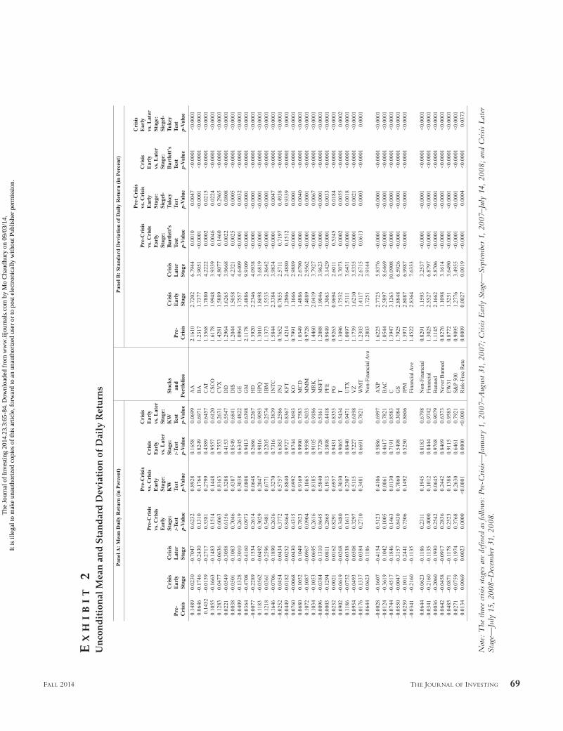
Mean Daily Returns

Panels A and B of Exhibit 2 present the arithmetic mean and the standard deviation of the percentage (non-annualized) daily returns for the 31 sample stocks, the equally weighted portfolio of the 26 non-financial stocks (Non-Financial), 5 financial stocks (Financial), 8 sample stocks (Banned)4 that were subjected to a blanket short-selling ban by the SEC at some time during the later stage of the crisis period and those that were not (Never Banned), all 31 stocks (EW31), the S&P 500, and the risk-free rate. The daily risk-free rate here is calculated as 1/365th of the per-annum percentage yield on the constant maturity three-month maturity Treasury bills. The Banned and Never Banned portfolios are formed to see whether the blanket short-selling ban had the desired impact on stock returns.

To see if the inter-period mean differences are sta-tistically significant, Exhibit 2 contains the p-values of the parametric t-test and the non-parametric Kruskal–Wallis (KW) test. For testing inter-period differences in the standard deviation, the p-values of the parametric Bartlett test and the non-parametric Siegel–Tukey test are provided. The t-test p-value is two sided with equal variance, and the chi-square p-values for the Kruskal–Wallis, Bartlett, and Siegel–Tukey tests are all one sided.

Representing the overall U.S. market, the average daily percentage return on the S&P 500 was positive (+0.0271) in the pre-crisis period, turned negative in the early stage of the crisis period (−0.0759), and sank deeper (−0.1974) in the later stage of the crisis. The EW31 portfolio (+0.0485, −0.0871, −0.1178) and the Non-Financial portfolio (+0.0644, −0.0623, –0.1186)

The

Jou

rnal

of

Inve

stin

g 20

14.2

3.3:

65-8

4. D

ownl

oade

d fr

om w

ww

.iijo

urna

ls.c

om b

y M

o C

haud

hury

on

09/0

3/14

.It

is il

lega

l to

mak

e un

auth

oriz

ed c

opie

s of

this

art

icle

, for

war

d to

an

unau

thor

ized

use

r or

to p

ost e

lect

roni

cally

with

out P

ublis

her

perm

issi

on.


EX

HI

BI

T 2

Un

con

dit

ion

al M

ean

an

d S

tan

dar

d D

evia

tion

of

Dai

ly R

etu

rns

Not

e: T

he th

ree

cris

is st

ages

are

def

ined

as

follo

ws:

Pre

-Cris

is—

Janu

ary

1, 2

007–

Aug

ust 3

1, 2

007;

Cris

is E

arly

Sta

ge—

Sept

embe

r 1,

2007

–Jul

y 14

, 20

08;

and

Cris

is L

ater

St

age—

July

15,

200

8–D

ecem

ber 3

1, 2

008.

The

Jou

rnal

of

Inve

stin

g 20

14.2

3.3:

65-8

4. D

ownl

oade

d fr

om w

ww

.iijo

urna

ls.c

om b

y M

o C

haud

hury

on

09/0

3/14

.It

is il

lega

l to

mak

e un

auth

oriz

ed c

opie

s of

this

art

icle

, for

war

d to

an

unau

thor

ized

use

r or

to p

ost e

lect

roni

cally

with

out P

ublis

her

perm

issi

on.


exhibit the same pattern.5 The Financial portfolio, however, shows a somewhat different pattern (–0.0341, –0.2160, –0.1135) in that the daily average loss abated in the later stage of the crisis.

The Never Banned portfolio (of stocks never sub-jected to the shorting ban) behaves largely the same way as the Non-Financial portfolio, while the Banned portfolio (of stocks subjected to shorting ban) largely resembles the Financial portfolio.

From a statistical point of view, as indicated by the t-test and Kruskal–Wallis test, the inter-period dif-ferences in the mean daily returns are not significant at the conventional significance levels, possibly due to the behavior of the standard deviations, to be discussed momentarily.

Several observations are worth noting about the mean returns evidence. First, the U.S. stock market seems to have reacted to the housing and mortgage sector troubles in an incremental fashion and at a rather slow speed. Second, as expected, the Wall Street heavy-weights were affected quite badly. Third, the mean daily return of the Non-Financial and Financial portfolios in the later stage of the crisis was very close, –0.1186% and –0.1135% respectively, but their cumulative returns were not, –18.39% and –33.73%. This lends support to studying the daily returns separately during the crisis period and also underscores the importance of exam-ining the higher-order moments and quantiles.

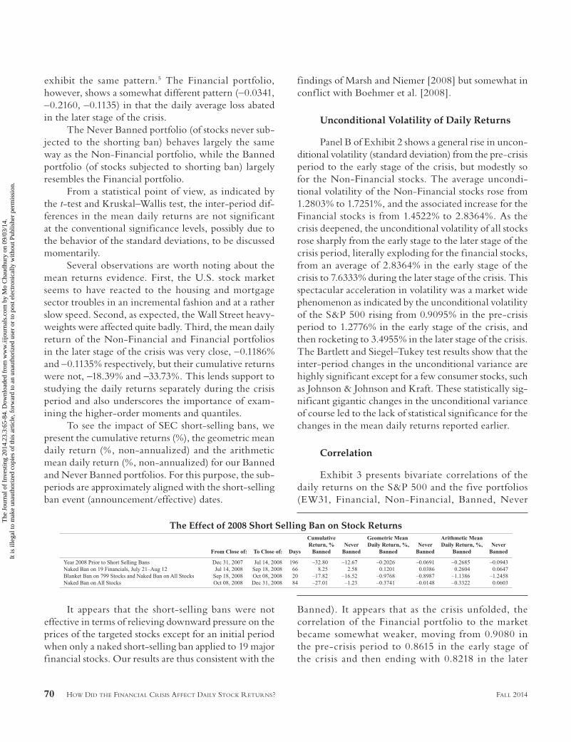
To see the impact of SEC short-selling bans, we present the cumulative returns (%), the geometric mean daily return (%, non-annualized) and the arithmetic mean daily return (%, non-annualized) for our Banned and Never Banned portfolios. For this purpose, the sub-periods are approximately aligned with the short-selling ban event (announcement/effective) dates.

findings of Marsh and Niemer [2008] but somewhat in conf lict with Boehmer et al. [2008].

Unconditional Volatility of Daily Returns

Panel B of Exhibit 2 shows a general rise in uncon-ditional volatility (standard deviation) from the pre-crisis period to the early stage of the crisis, but modestly so for the Non-Financial stocks. The average uncondi-tional volatility of the Non-Financial stocks rose from 1.2803% to 1.7251%, and the associated increase for the Financial stocks is from 1.4522% to 2.8364%. As the crisis deepened, the unconditional volatility of all stocks rose sharply from the early stage to the later stage of the crisis period, literally exploding for the financial stocks, from an average of 2.8364% in the early stage of the crisis to 7.6333% during the later stage of the crisis. This spectacular acceleration in volatility was a market wide phenomenon as indicated by the unconditional volatility of the S&P 500 rising from 0.9095% in the pre-crisis period to 1.2776% in the early stage of the crisis, and then rocketing to 3.4955% in the later stage of the crisis. The Bartlett and Siegel–Tukey test results show that the inter-period changes in the unconditional variance are highly significant except for a few consumer stocks, such as Johnson & Johnson and Kraft. These statistically sig-nificant gigantic changes in the unconditional variance of course led to the lack of statistical significance for the changes in the mean daily returns reported earlier.

Correlation

Exhibit 3 presents bivariate correlations of the daily returns on the S&P 500 and the f ive portfolios (EW31, Financial, Non-Financial, Banned, Never

It appears that the short-selling bans were not effective in terms of relieving downward pressure on the prices of the targeted stocks except for an initial period when only a naked short-selling ban applied to 19 major financial stocks. Our results are thus consistent with the

Banned). It appears that as the crisis unfolded, the correlation of the Financial portfolio to the market became somewhat weaker, moving from 0.9080 in the pre-crisis period to 0.8615 in the early stage of the crisis and then ending with 0.8218 in the later

The Effect of 2008 Short Selling Ban on Stock Returns

The

Jou

rnal

of

Inve

stin

g 20

14.2

3.3:

65-8

4. D

ownl

oade

d fr

om w

ww

.iijo

urna

ls.c

om b

y M

o C

haud

hury

on

09/0

3/14

.It

is il

lega

l to

mak

e un

auth

oriz

ed c

opie

s of

this

art

icle

, for

war

d to

an

unau

thor

ized

use

r or

to p

ost e

lect

roni

cally

with

out P

ublis

her

perm

issi

on.


stage of the crisis. The market correlation of the Non- Financial portfolio, of course, shows the opposite trend, increasing from 0.9612 to 0.9700 and then to 0.9821 over the respective periods. This differential course is more vividly shown by the bivariate cor-relation of the Financial and Non-Financial portfo-lios. This correlation started at 0.8280 in the pre-crisis period, declined to 0.8004 in the early stage of the

crisis, and then further weakened to 0.7656 in the later stage of the crisis.

Beta, R-Squared, and Alpha

We estimate the following market model regres-sion separately for the pre-crisis period and the early and later stage of the crisis period:

E X H I B I T 3Unconditional Correlation of Daily Returns for Six Portfolios

The

Jou

rnal

of

Inve

stin

g 20

14.2

3.3:

65-8

4. D

ownl

oade

d fr

om w

ww

.iijo

urna

ls.c

om b

y M

o C

haud

hury

on

09/0

3/14

.It

is il

lega

l to

mak

e un

auth

oriz

ed c

opie

s of

this

art

icle

, for

war

d to

an

unau

thor

ized

use

r or

to p

ost e

lect

roni

cally

with

out P

ublis

her

perm

issi

on.


Market Model Regression:

Daily Excess Return = Alpha + Beta × Daily Excess S&P 500 Return

Furthermore, to see if the changes in alpha and beta between the periods are statistically significant, we estimate the following two regressions:

Regression A:

Daily Excess Return = Alpha Pre-Crisis + Change in Alpha × Dum1 + Beta Pre-Crisis × Daily Excess S&P 500 Return + Change in Beta × Daily Excess S&P 500 Return × Dum1,

andRegression B:

Daily Excess Return = Alpha Early + Change in Alpha Early × Dum2 + Beta Early × Daily Excess S&P 500 Return + Change in Beta Early × Daily Excess S&P 500 Return × Dum2,

where Dum1 = 0 during January 1, 2007–August 31, 2007, and Dum1 = 1 otherwise during the estima-tion period January 1, 2007–July 14, 2008, for A, and Dum2 = 0 during September 1, 2007–July 14, 2008, and Dum2 = 1 otherwise, during the estimation period September 1, 2007–December 31, 2008, for B. The results for the market model regression are presented in Exhibit 4, and those for changes in the parameters are reported in Exhibit 5. The t-statistics in both exhibits are calculated using heteroskedasticity and autocorrelation consistent standard errors.

The pre-crisis period results in Exhibit 4 indicate that on average the beta of the non-financial stocks rose only slightly from 0.8762 in the pre-crisis period to 0.8802 in the early going of the crisis and then moved to a somewhat higher level of 0.9142 in the later stage of the crisis. The t-statistic figures in Exhibit 5 for the individual non-financial stocks show a mixed picture of statistical significance of the beta changes at conven-tional levels.

In contrast, as the larger (than market) increase in the unconditional volatility outweighed the drop in the correlation with the market, the average beta of the financial stocks rose sharply from 1.3003 in the pre-crisis period to 1.7213 during the early stage of the crisis and

then subsided somewhat to 1.6173 in the later stage of the crisis period.6 Except for Goldman Sachs, the rise in beta of the financial stocks in the early stage of the crisis is statistically significant at conventional levels. The subsequent change in beta, of a lesser magnitude, in the later stage of the crisis is not statistically significant except for AXP.

To summarize, during the course of the crisis, the beta risk of the financial stocks rose 24.38% in contrast to 4.34% rise in the case of the non-financial stocks. Accordingly, it seems that the financial crisis consider-ably widened the equity cost differential of the financial corporations over the non-financial corporations. This result is quite important because the financial institu-tions were badly in need of raising equity capital at a time when they had a decided cost disadvantage com-pared with the non-financial stocks, and this was so in an environment of severe scarcity of capital.

As the relative importance of market risk is com-monly measured by the R-squared of market model regression, we now examine the R-squared results in Exhibit 4. As the financial crisis evolved, the average R-squared for the non-financial stocks continued to rise, reaching a substantially higher level of 69.36% in the later stage of the crisis. In contrast, the average R-squared of financial stocks experienced an overall decline ending at a level of 56.54% in the later stage of the crisis. The pattern at the individual stock level is largely similar as well.

It seems that the financial crisis led to a notable rise in the market risk and an even sharper rise in the non-market (industry- and/or security-specific) risk of the financial stocks. Accordingly, the total risk (uncon-ditional variance) of the individual f inancial stocks exploded with the market becoming a less dominant source of risk for these stocks despite wild f luctuations in the broader market during the f inancial crisis. In contrast, the market became a more important source of risk for the individual non-financial stocks as their non-market risk did not change much and their total risk shot up mostly because of the heightened market volatility.

Despite the gloomy consequences of the increase in total, market, and non-market risk for the financial stocks, it turns out that the financial crisis did not adversely affect their investment performance, as measured by the Jensen’s alpha from market model regression. The average alpha for these stocks, same as the alpha of the

The

Jou

rnal

of

Inve

stin

g 20

14.2

3.3:

65-8

4. D

ownl

oade

d fr

om w

ww

.iijo

urna

ls.c

om b

y M

o C

haud

hury

on

09/0

3/14

.It

is il

lega

l to

mak

e un

auth

oriz

ed c

opie

s of

this

art

icle

, for

war

d to

an

unau

thor

ized

use

r or

to p

ost e

lect

roni

cally

with

out P

ublis

her

perm

issi

on.


EX

HI

BI

T 4

Mar

ket

Mod

el R

egre

ssio

n R

esu

ltsThe

Jou

rnal

of

Inve

stin

g 20

14.2

3.3:

65-8

4. D

ownl

oade

d fr

om w

ww

.iijo

urna

ls.c

om b

y M

o C

haud

hury

on

09/0

3/14

.It

is il

lega

l to

mak

e un

auth

oriz

ed c

opie

s of

this

art

icle

, for

war

d to

an

unau

thor

ized

use

r or

to p

ost e

lect

roni

cally

with

out P

ublis

her

perm

issi

on.


EX

HI

BI

T 5

Reg

ress

ion

Res

ult

s fo

r C

han

ges

in M

ark

et M

odel

Par

amet

ers

Not

es:

Thi

s ex

hibi

t pre

sent

s re

sults

for R

egre

ssio

n A

and

B,

as s

how

n in

the

artic

le te

xt.

The

t-st

atist

ics a

re c

alcu

late

d us

ing

hete

rosk

edas

ticity

and

aut

ocor

rela

tion

cons

isten

t sta

ndar

d er

rors

. T

he th

ree

cris

is st

ages

are

def

ined

as

follo

ws:

Pre

-Cris

is—

Janu

ary

1, 2

007–

Aug

ust 3

1, 2

007;

Cris

is E

arly

Sta

ge—

Sept

embe

r 1,

2007

–Jul

y 14

, 20

08;

and

Cris

is L

ater

Sta

ge—

July

15,

20

08—

Dec

embe

r 31,

200

8.

The

Jou

rnal

of

Inve

stin

g 20

14.2

3.3:

65-8

4. D

ownl

oade

d fr

om w

ww

.iijo

urna

ls.c

om b

y M

o C

haud

hury

on

09/0

3/14

.It

is il

lega

l to

mak

e un

auth

oriz

ed c

opie

s of

this

art

icle

, for

war

d to

an

unau

thor

ized

use

r or

to p

ost e

lect

roni

cally

with

out P

ublis

her

perm

issi

on.


Financial Portfolio, is –0.0653 in the pre-crisis period. The average alpha declined further to –0.0804 during the early stage of the crisis, driven by the sharp rise in beta in this period, but then turned around and increased dramatically to +0.2072 in the later stage of the crisis, aided only somewhat by the concurrent modest fall in their beta.7 In comparison, the non-financial stocks start as the better performing group with an average alpha of +0.0391 in the pre-crisis period, they lost some shine in the early going of the crisis as indicated by their average alpha of +0.0036 in this period, and then rallied to an average alpha of +0.0616 in the later stage of the crisis. As noted previously, their beta risk increased at a mod-erate pace during these periods. This shows that the crisis led to an increased cost of equity and hence nega-tive mean daily returns for the leading U.S. stocks due to enhanced beta risk, but they still beat the market and other stocks on a market risk-adjusted basis. Given that the causes of the crisis concerned primarily the finan-cial institutions, the relative investment strength of the financial stocks, especially BAC, C, and JPM, is rather puzzling, at least at first glance.

Dynamics of Conditional Variance

To capture the dynamics of stochastically evolving conditional variance, we estimate slightly modif ied versions of two well-known discrete time conditional variance models, the GARCH (1,1) in mean and the EGARCH (1,1) in mean.

Return Equation:

ln[R(t + 1)] – ln[Rf (t + 1)] = α + β {ln[R

m(t + 1)]

− ln[Rf (t + 1)]} + λ√h(t + 1) + ε(t + 1) √h(t + 1)

whereR = 1 plus the daily total return in decimalR

m = 1 plus the daily total return on the market

(S&P 500) in decimalR

f = 1 plus the constant maturity three-month

Treasury rate expressed in decimal on a daily (365 days, APR) basis

ε∼N(0,1) and assumed i.i.d.

Conditional Variance Equation:

GARCH (1,1): h(t + 1) = β0 + β

1 h(t) + β

2 ε2(t)

EGARCH (1,1): ln[h(t + 1)] = β0 + β

1 ln[h(t)]

+ β2 {γ ε(t) + |ε(t)| − E(|ε(t)|)}

In the GARCH variance equation, β2 ref lects the

symmetric heteroskedasticity effect of the size of the return innovation on the conditional variance, while β

1

captures the autoregressive effect in conditional vari-ance. The measure of persistence in variance is β

1 + β

2.

The EGARCH specification does not require non-negativity constraints and allows leverage effect, namely, higher (lower) volatility and falling (rising) prices go hand in hand. In the variance equation for EGARCH, E(|ε(t)|= √(2π), given the assumption ε∼N(0,1). The parameter γ is known as the leverage parameter and the product β

2 γ as the leverage effect. If different from

0.0, γ creates an asymmetric effect of return innovation on the conditional variance. If β

2 and γ are of opposite

signs (β2 γ < 0), then a negative (positive) return inno-

vation leads to an increase (decrease) in the conditional variance.

In these specif ications, we have modif ied the standard GARCH and EGARCH in mean models by incorporating the excess log return on the market as an additional explanatory variable in the return equation.

Exhibit 6 presents the GARCH model results. For the S&P 500, the financial crisis led to a more persistent variance process, with the measure of persistence rising from 0.9254 in the pre-crisis period to 0.9724 in the later stage of the crisis period. This increased persistence appears to have been driven by a marked increase in the effect of the most recent asset price innovation, as cap-tured by the increase in the ARCH parameter β

2, from

0.0692 in the pre-crisis period to 0.1501 in the later stage of the crisis period. Similar to the S&P 500, the finan-cial stocks portfolio and the individual financial stocks experienced a significant rise in variance persistence as the crisis unfolded. Except or Goldman Sachs, the driver of the increase in variance persistence is a sharp rise in the value of the GARCH parameter β

1, meaning that the

cumulative effect of large swings in these stocks played a more dominant role as the crisis deepened. This is perhaps because the financial stocks were constantly in news during the crisis period, and as such, in the later stage of the crisis period, the latest news did not impact the already elevated stock variance as badly.

In contrast, the portfolio of non-financial stocks showed a sharp decline in variance persistence, from 0.9430 in the pre-crisis period to 0.4806 in the later stage of the crisis period, with a decrease in the GARCH parameter β

1 (from 0.8678 to 0.2105) outpacing the

increase in the ARCH parameter β2 (from 0.0752 to

The

Jou

rnal

of

Inve

stin

g 20

14.2

3.3:

65-8

4. D

ownl

oade

d fr

om w

ww

.iijo

urna

ls.c

om b

y M

o C

haud

hury

on

09/0

3/14

.It

is il

lega

l to

mak

e un

auth

oriz

ed c

opie

s of

this

art

icle

, for

war

d to

an

unau

thor

ized

use

r or

to p

ost e

lect

roni

cally

with

out P

ublis

her

perm

issi

on.


0.2702). The individual non-financial stocks, however, show varied patterns. As one would expect, the vari-ance persistent effect for the portfolio of non-banned (banned) stocks is similar to that of the non-financial (financial) stocks.

We do not observe any discernible pattern in the conditional volatility risk premium parameter λ either for the f inancial or the non-financial stocks. This is rather surprising given that the markets were gripped by fear during the crisis as evidenced by the sharp rise in the VIX level.

The GARCH results are based on a conditional normal distribution for the excess return innovation.

To see the effect of a fatter-tail conditional distribu-tion, we also generated GARCH results for a conditional t-distribution with κ degrees of freedom; the inverse of the degrees of freedom, that is, 1/κ is estimated jointly as an additional parameter.8 We do not report the results here as they are largely similar to the previous results for the normal GARCH.

In Exhibit 7, we report the estimated leverage effect along with results for other parameters. For the S&P 500, the leverage effect is of conventional type prior to the crisis (β

2γ = −0.2976) and in the later stage

of the crisis (β2γ = −0.3494) but not during the early

stage of the crisis (β2γ = +0.1820). Overall, the leverage

E X H I B I T 6Conditional Variance Process: Stationary GARCH (1, 1) in Mean, Conditional Normal Distribution

Notes: This exhibit presents results using the Return Equation and Conditional Variance Equation, as shown in the article text. The three crisis stages are defined as follows: Pre-Crisis—January 1, 2007–August 31, 2007; Crisis Early Stage—September 1, 2007–July 14, 2008; and Crisis Later Stage—July 15, 2008—December 31, 2008.

The

Jou

rnal

of

Inve

stin

g 20

14.2

3.3:

65-8

4. D

ownl

oade

d fr

om w

ww

.iijo

urna

ls.c

om b

y M

o C

haud

hury

on

09/0

3/14

.It

is il

lega

l to

mak

e un

auth

oriz

ed c

opie

s of

this

art

icle

, for

war

d to

an

unau

thor

ized

use

r or

to p

ost e

lect

roni

cally

with

out P

ublis

her

perm

issi

on.


Not

es:

Thi

s ex

hibi

t pre

sent

s re

sults

usin

g th

e R

etur

n E

quat

ion

and

Con

ditio

nal V

aria

nce

Equ

atio

n, a

s sh

own

in th

e ar

ticle

text

. T

he th

ree

cris

is st

ages

are

def

ined

as

follo

ws:

Pre

-Cris

is—

Janu

ary

1, 2

007–

Aug

ust 3

1, 2

007;

Cris

is E

arly

Sta

ge—

Sept

embe

r 1,

2007

–Jul

y 14

, 20

08;

and

Cris

is L

ater

Sta

ge—

July

15,

200

8—D

ecem

ber 3

1, 2

008.

EX

HI

BI

T 7

Est

imat

ed L

ever

age

Eff

ect:

Con

dit

ion

al V

aria

nce

Pro

cess

—S

tati

onar

y E

GA

RC

H (1

, 1) i

n M

ean

, Con

dit

ion

al N

orm

al D

istr

ibu

tion

The

Jou

rnal

of

Inve

stin

g 20

14.2

3.3:

65-8

4. D

ownl

oade

d fr

om w

ww

.iijo

urna

ls.c

om b

y M

o C

haud

hury

on

09/0

3/14

.It

is il

lega

l to

mak

e un

auth

oriz

ed c

opie

s of

this

art

icle

, for

war

d to

an

unau

thor

ized

use

r or

to p

ost e

lect

roni

cally

with

out P

ublis

her

perm

issi

on.


effect in the S&P 500 became only somewhat stronger when the crisis deepened in the fall of 2008 compared with the pre-crisis period. Among the non-financial stocks, we do not see any clear evidence of a leverage effect prior to the crisis and in the early stage of the crisis as indicated by many positive as well as negative values of β

2γ. But 19 out of 26 of these stocks exhibit a

leverage effect in the later stage of the crisis. The finan-cial stocks also indicate a strengthening leverage effect moving through the crisis period.

Unconditional Skewness and Kurtosis of Daily Returns

Panel A of Exhibit 8 reports the traditional mea-sure of skewness, namely, average cubed deviation (from the sample mean)/cubed standard deviation. However, sample outliers may have a disproportionate effect on this measure of skewness. As such, Panel B of Exhibit 10 reports an alternative measure of skewness, namely, 3 (Mean − median)/standard deviation. Values of both measures are expected to be negative (positive) for left (right) or negatively (positively) skewed distributions. Prior to the financial crisis, the unconditional distribu-tion of daily stock returns of most individual stocks as well as the various portfolios including the S&P 500 was characterized by negative skewness, according to both measures of skewness. In the early stage of the financial crisis, however, many individual stocks, especially the financial stocks, as well as the S&P 500, became posi-tively skewed (or less negatively skewed) according to the traditional measure and less negatively skewed according to the alternative measure. This pattern became stronger for many non-financial stocks and the S&P 500 during the later stage of the crisis; the financial stocks remained positively skewed although the extent of positive skew abated somewhat for them, according to the traditional measure.

Thus, the crisis made the unconditional distribu-tion of the S&P 500 more symmetric around the lower (and negative) mean. As many individual stocks in fact became positively skewed, the lower average daily return in the crisis period is not merely due to a few outlier negative returns.

Let us next look at the unconditional physical kur-tosis results in Panel C of Exhibit 8. There does not appear to be any clear pattern of change in the physical

kurtosis during either stage of the crisis for the indi-vidual financial or non-financial stocks. For the portfo-lios including the S&P 500, it appears that the physical kurtosis dropped during the early stage of the crisis and then partly rebounded during the later stage of the crisis. Overall, from the pre-crisis period to the later stage of the crisis, the unconditional (excess) physical kurtosis declined somewhat (from +2.4946 to +2.2557) for the Non-Financial portfolio, increased sizably (from +1.9223 to +2.4649) for the Financial portfolio, and dropped noticeably (from +2.2582 to +1.4251) for the S&P 500.

Tail Risk

In many applications including the estimation of regulatory and economic capital for trading portfolios and the associated question of capital adequacy for finan-cial institutions, the tail risk or the chances of extreme asset price moves is most consequential. The literature on tail risk measurement is extensive and quite sophisti-cated.9 In this article, we simply report the 5th percentile (95% VaR) and the first percentile (99% VaR) of the empirical unconditional distribution of daily returns as our measures of tail risk. In keeping with practice, we assume zero unconditional mean for the daily returns in VaR estimation.

Exhibit 9 presents the 95% VaR in Panel A and the 99% VaR in Panel B, and the worst returns in Panel C. Focusing on the 99% VaR, the most traditional market risk measure, the tail risk of the Non-Financial port-folio rose from −2.4011% in the pre-crisis period to −2.7347% in the early stage of the crisis and jumped to −7.6084% in the later stage of the crisis. As expected, the changes are quite dramatic for the Financial portfolio, from −3.7088% in the pre-crisis period to −5.0217% in the early stage of the crisis and then onto a whopping −14.8282% in the later stage of the crisis. The broader market tail risk, represented by that of the S&P 500, also shot up significantly, as indicated by the 99% VaR figures of −2.7597% (pre-crisis), −2.9369% (early stage of crisis), and −8.9043% (later stage of crisis). Stated differently, the tail risk in the later stage of the crisis was about 3.17 times, 4.0 times, and 3.23 times the pre-crisis tail risk for the Non-Financial, Financial, and the broader market portfolios, respectively.

The

Jou

rnal

of

Inve

stin

g 20

14.2

3.3:

65-8

4. D

ownl

oade

d fr

om w

ww

.iijo

urna

ls.c

om b

y M

o C

haud

hury

on

09/0

3/14

.It

is il

lega

l to

mak

e un

auth

oriz

ed c

opie

s of

this

art

icle

, for

war

d to

an

unau

thor

ized

use

r or

to p

ost e

lect

roni

cally

with

out P

ublis

her

perm

issi

on.


Several observations are in order. First, as is well known and confirmed by our evidence, it is more pru-dent to use historical simulation over a period that is stressful rather than benign. In this sense, the new Basel

rule (BCBS [2009]) of adding a stress period VaR makes sense.

Second, volatility implied from derivative prices seems most promising in capturing the pending tail risk.

E X H I B I T 8Skewness and Kurtosis of Daily Returns (in %)

Notes: The three crisis stages are defined as follows: Pre-Crisis—January 1, 2007–August 31, 2007; Crisis Early Stage—September 1, 2007–July 14, 2008; and Crisis Later Stage—July 15, 2008—December 31, 2008.

The

Jou

rnal

of

Inve

stin

g 20

14.2

3.3:

65-8

4. D

ownl

oade

d fr

om w

ww

.iijo

urna

ls.c

om b

y M

o C

haud

hury

on

09/0

3/14

.It

is il

lega

l to

mak

e un

auth

oriz

ed c

opie

s of

this

art

icle

, for

war

d to

an

unau

thor

ized

use

r or

to p

ost e

lect

roni

cally

with

out P

ublis

her

perm

issi

on.


E X H I B I T 9Extreme Percentiles of Daily Returns

Notes: The three crisis stages are defined as follows: Pre-Crisis—January 1, 2007–August 31, 2007; Crisis Early Stage—September 1, 2007–July 14, 2008; and Crisis Later Stage—July 15, 2008—December 31, 2008.

The

Jou

rnal

of

Inve

stin

g 20

14.2

3.3:

65-8

4. D

ownl

oade

d fr

om w

ww

.iijo

urna

ls.c

om b

y M

o C

haud

hury

on

09/0

3/14

.It

is il

lega

l to

mak

e un

auth

oriz

ed c

opie

s of

this

art

icle

, for

war

d to

an

unau

thor

ized

use

r or

to p

ost e

lect

roni

cally

with

out P

ublis

her

perm

issi

on.


EX

HI

BI

T 1

0E

xtre

me

Per

cen

tile

s of

Dai

ly R

etu

rns

(in

%) i

n T

erm

s of

Sta

nd

ard

Dev

iati

on

Not

es:

Pane

ls A

, B

and

C re

port

scal

ing

by th

e sa

me

perio

d st

anda

rd d

evia

tion,

and

Pan

els

D,

E a

nd F

repo

rt sc

alin

g by

the

pre-

cris

is st

anda

rd d

evia

tion.

The

thre

e cr

isis

stag

es a

re d

efin

ed

as fo

llow

s: P

re-C

risis

—Ja

nuar

y 1,

200

7–A

ugus

t 31,

200

7; C

risis

Ear

ly S

tage

—Se

ptem

ber 1

, 20

07–J

uly

14,

2008

; an

d C

risis

Lat

er S

tage

—Ju

ly 1

5, 2

008—

Dec

embe

r 31,

200

8.

The

Jou

rnal

of

Inve

stin

g 20

14.2

3.3:

65-8

4. D

ownl

oade

d fr

om w

ww

.iijo

urna

ls.c

om b

y M

o C

haud

hury

on

09/0

3/14

.It

is il

lega

l to

mak

e un

auth

oriz

ed c

opie

s of

this

art

icle

, for

war

d to

an

unau

thor

ized

use

r or

to p

ost e

lect

roni

cally

with

out P

ublis

her

perm

issi

on.


To match the daily 99% VaR level of the S&P 500 portfolio during the entire later stage of the crisis, one would have needed an annualized volatility level of 60.7613%. This level was reached by the S&P 500 implied volatility average around October 09, 2008. In fact, a better route is perhaps to use the average implied volatility of in the money call (out of the money put) options. This high delta (low strike) implied vola-tility average exploded to above the required 60% level on September 29, 2008, the third worst day for the S&P 500 during the later stage of the crisis, and then exploded further to above 70% on October 09, 2008. Of course, there were ups and downs, but the implied volatility moving average would have still remained quite high.

Third, it was a failure to forecast the level of vola-tility (and not the VaR method), that is at the heart of market risk capital inadequacy experienced by many financial institutions. To see this, Panels A, B, and C (D, E, and F) of Exhibit 10 present the 95% VaR, 99% VaR, and the worst daily return in the pre-crisis period and the early and later stages of the crisis in terms of the unconditional standard deviation of daily return in the respective (pre-crisis) periods.

Panels A and B of Exhibit 10 indicate that with a reasonably accurate forecast of the unconditional vola-tility, the use of VaR with a simple i.i.d. normal dis-tribution is likely to produce fairly good tail risk and capital requirement. The 95% (99%) VaR figures for the Financial, Non-Financial, and S&P 500 portfolios during the later stage of the crisis are equal to 1.6504 (2.3384), 1.5805 (2.1553), and 1.7459 (2.5474) times

is a Black Swan event according to non-crisis experi-ence appears pretty mundane (like a normal distribu-tion event) when measured in terms of the same period standard deviation.

SUMMARY AND CONCLUSIONS

In this article, we examined the behavior of 31 major U.S. stocks, some equally weighted portfolios constructed from these stocks, and the S&P 500 during the recent financial crisis using daily return data from January 1, 2007, to December 31, 2008. As such the study produces essential clues to the implication of rare events for a wide range of applications that would be of interest to researchers and practitioners including fund managers, financial insti-tutions, and exchanges and their regulators.

Consistent with the large cumulative declines in stock prices, the mean daily returns deteriorated consid-erably, especially for the financial stocks starting in the early stage of the crisis. In line with Marsh and Niemer [2008], but in conf lict with Boehmer et al. [2008], we find that only the initial naked short-selling ban that was limited to 19 major financial stocks (5 included in our sample) had some desired impact of relieving the down-ward pressure on the prices of the targeted stocks.

As expected, the most sizable impact of the crisis was on the unconditional standard deviation of daily returns that shot up to more than three times the pre-crisis level for the non-financial stocks, four times for the S&P 500, and five times for the financial stocks. The correlation between the portfolios of the financial stocks and the non-financial stocks actually decreased during

Just using the implied volatility and a normal distribu-tion, tail risk can be estimated much more accurately and dynamically. To see this, following are the daily non-annualized 99% VaR for the S&P 500 portfolio from Exhibit 9 and the required level of the annualized standard deviation to match this level of tail risk using an independent and identically distributed normal with mean 0.0.

the same period standard deviations respectively, not too far from the 1.6450 (2.3263) standard deviations corresponding to the normal distribution. But Panels D and E of Exhibit 10 show that the 95% and 99% VaR of the actual empirical distribution in the later stage of the crisis are in excess of six pre-crisis or normal period standard deviations, a phenomenon popularly known as a “Black Swan” event. In other words, what

The

Jou

rnal

of

Inve

stin

g 20

14.2

3.3:

65-8

4. D

ownl

oade

d fr

om w

ww

.iijo

urna

ls.c

om b

y M

o C

haud

hury

on

09/0

3/14

.It

is il

lega

l to

mak

e un

auth

oriz

ed c

opie

s of

this

art

icle

, for

war

d to

an

unau

thor

ized

use

r or

to p

ost e

lect

roni

cally

with

out P

ublis

her

perm

issi

on.


the crisis. Previously, Ang and Bekaert [2002], among others, reported increased correlation of international equity markets in falling markets with higher volatility. Longin and Solnik [2001] reported that correlation of equity markets is related to market trend and not vola-tility, rising in bear markets, but not in bull markets. Our evidence for the U.S. internal market thus indicates that home diversification benefits may actually be better than international diversification during times of crisis. This needs to be researched further, including the pos-sibility of a greater home bias during crisis time.

Because of sector-specif ic developments, the market risk became relatively less important for the financial stocks and the opposite is the case for the non-financial stocks. The beta risk of the non-financial stocks increased mildly, while that of the financial stocks rose significantly. Thus the cost of equity for the financial institutions increased markedly, making it more diffi-cult for them to raise the much-needed equity capital. Simultaneously, however, as the market risk became less important compared to the unique risk of the financials during the crisis, investors were better off retaining them for diversif ication purposes. This hedging demand is perhaps one of the factors why the financial stocks put up a stellar performance during the crisis, with their average alpha rising from –0.0653 in the pre-crisis period to a stunning +0.2072 in the later stage of the crisis. None-theless, the significant leap in the alpha of the financials remains puzzling.

Using the GARCH (1,1) in mean conditional vari-ance process, we noted a significant rise in variance per-sistence for the S&P 500 and the financial stocks as the crisis unfolded. For their part, the non-financial stocks show a mixed pattern. Using the EGARCH (1,1) in mean model, we find that the leverage effect in the later stage of the crisis is generally stronger than in the pre-crisis period, thus implying a rise in the unconditional left or negative skewness of returns. But considering the unprecedented extent of the crisis, the leverage effect was neither very strong nor very pervasive. Instead, we found a weaker negative skew to positive skew in the unconditional distributions during the later stage of the crisis. The unconditional kurtosis evidence is mixed at the individual stock level, but it dropped somewhat for the Non-Financial portfolio and rose for the Financial portfolio. These effects are not due to the short-selling bans as the bans did not exert much of an impact on the returns of the Banned stocks.

Additionally, the fit of the GARCH models weak-ened during the crisis, and the sharp rise in the market fear gauge, the VIX, was not ref lected in a rise in the conditional volatility risk premium. As the results are similar for the conditional t-distribution, these GARCH findings are not due to insufficient allowance for fatter tails. Our findings thus raise questions about the overall usefulness of GARCH models in capturing return dynamics during crisis periods and as such the utility of GARCH-based derivative valuation models for trading, marking to model, and other risk measure-ment and management purposes. As noted by Longin and Solnik [2001] and Ang and Bekaert [2002], the GARCH models cannot quite handle the asymmetries in returns behavior under regime shifts.

Lastly, the tail risk (99% VaR) of the Non-Finan-cial, Financial, and the S&P 500 portfolios in the later stage of the crisis was more than three times their tail risk in the pre-crisis period, driven primarily by the unprec-edented increase in the unconditional volatility. Con-trary to the belief of some, we find that it is the failure to forecast the unprecedented level of unconditional volatility and not the VaR measure or the normality assumption that led to the widespread underestimation of risk capital during the crisis.

Although a number of crisis effects or the lack thereof (correlation, Jensen’s alpha, leverage effect, con-ditional volatility risk premium, unconditional skew-ness and kurtosis, VaR) reported here seem anomalous, can these effects possibly be traced to the sharp rise in total risk in the sense of unconditional volatility? Decades of research emphasis on conditional volatility has deeply enriched our understanding of the role of stochastic nature of conditional volatility and the asso-ciated departures from normality. At the very least, the empirical f indings of this study provides some moti-vation for better forecasting of unconditional volatility during crisis periods and better modeling of innova-tions to unconditional volatility in risk and portfolio measurement and management as well as in derivative valuation models.

ENDNOTES

1GARCH = generalized autoregressive conditional het-eroskedasticity; EGARCH = exponential GARCH.

2See http://www.sec.gov/rules/other/2008/34-58166.pdf.

The

Jou

rnal

of

Inve

stin

g 20

14.2

3.3:

65-8

4. D

ownl

oade

d fr

om w

ww

.iijo

urna

ls.c

om b

y M

o C

haud

hury

on

09/0

3/14

.It

is il

lega

l to

mak

e un

auth

oriz

ed c

opie

s of

this

art

icle

, for

war

d to

an

unau

thor

ized

use

r or

to p

ost e

lect

roni

cally

with

out P

ublis

her

perm

issi

on.


3Pressured by a mounting bank run, the FDIC closed down IndyMac on July 12, 200, marking the largest U.S. bank closure since the closure of Continental Illinois in 1984. Two days later, a three-point plan to rescue the ailing mort-gage giants Fannie Mae and Freddie Mac was announced by U.S. Treasury Secretary Henry Paulson on July 14, 2008. Meantime, contagion of the crisis to the broader stock market became evident as the financial sector ETF (XLF) hit a clear new low on July 14, 2008, and the DJIA as well as the S&P 500 hit new lows on July 15, 2008. Fearing even a deeper crash in the stock market, the SEC, on July 15, 2008, announced a temporary naked short-selling ban on 19 major financial stocks.

4These eight stocks are the five financial stocks—AXP, BAC, C, GS, and JPM—and three non-financial stocks—GE, GM and IBM.

5Consumer stocks such as McDonald’s, Proctor & Gamble, and Wal-Mart appeared to have bucked this down-ward trend in daily returns.

6By construction, the Non-Financial and Financial portfolios share the same beta levels and patterns of the corresponding averages but not necessarily the statistical significance.

7At the individual stock level, among the financial stocks, C, BAC, and JPM showed improvement in alpha performance over the entire period while AXP and GS deteriorated.

8As κ tends to infinity, the t distribution approaches the normal distribution.

9Please see Malevergne and Sornette [2006].

REFERENCES

Ang, A., and G. Bekaert. “International Asset Allocation with Regime Shifts.” Review of Financial Studies, Vol. 15, No.4 (2002), pp. 1137-1187.

Bartram, S.M., and G.M. Bodnar. “No Place to Hide: The Global Crisis in Equity Markets in 2008/09.” Journal of Inter-national Money and Finance, Vo. 28, No. 8 (2009), pp. 1246-1292.

BCBS. “Revisions to the Basel II Market Risk Framework, Basel Committee on Banking Supervision.” Bank for Inter-national Settlements, 2009. Available at http://www.bis.org/publ/bcbs158.htm.

Boehmer, E., C.M. Jones, and X. Zhang. “Shackling Short Sellers: The 2008 Shorting Ban.” Working paper, Columbia University, 2008. Available at http://www2.gsb.columbia.edu/faculty/cjones/ShortingBan.pdf.

Dwyer, G.P., and P. Tkac. “The Financial Crisis of 2008 in Fixed-Income Markets.” Journal of International Money and Finance, Vol. 28, No. 8 (2009), pp. 1293-1316.

Gorton, G. “The Panic of 2007.” Federal Reserve Bank of Kansas City’s Jackson Hole Conference, August, 2008. Available at http://www.kc.frb.org/publicat/sympos/2008/gorton.08.04.08.pdf.

Kho, B.-C., and R. Stulz. “Banks, the IMF, and the Asian Crisis.” Working paper, Seoul National University, 1999.

Lioui, A. “The Undesirable Effects of Banning Short Sales.” Working paper, EDHEC Risk and Asset Management Research Centre, 2009.

Lo, A. “Reading About the Financial Crisis: A 21-Book Review.” Working paper, MIT Sloan School of Manage-ment, 2012.

Longin, F., and B. Solnik. “Extreme Correlation of Inter-national Equity Markets.” Journal of Finance, Vol. 56, No.2 (2001), pp. 649-676.

Longstaff, F.A. “The Subprime Credit Crisis and Contagion in Financial Markets.” Working paper, UCLA Anderson School and NBER, 2008.

Malevergne, Y., and D. Sornette. Extreme Financial Risks: From Dependence to Risk Management. Springer, 2006.

Marsh, I.W., and N. Niemer. “The Impact of Short Sales Restrictions.” Industry study, International Securities Lending Association (ISLA), Alternative Investment Manage-ment Association (AIMA), and London Investment Banking Association (LIBA), 2008.

Phillips, P.C.B., and J. Yu. “Dating the Timeline of Financial Bubbles during the Subprime Crisis.” Quantitative Economics, Vol. 2, No. 3 (2011), pp. 455-491.

Schwert, W.G. “Stock Volatility during the Recent Finan-cial Crisis.” Working Paper No. 16976, National Bureau of Economic Research, 2011.

To order reprints of this article, please contact Dewey Palmieri at [email protected] or 212-224-3675.

The

Jou

rnal

of

Inve

stin

g 20

14.2

3.3:

65-8

4. D

ownl

oade

d fr

om w

ww

.iijo

urna

ls.c

om b

y M

o C

haud

hury

on

09/0

3/14

.It

is il

lega

l to

mak

e un

auth

oriz

ed c

opie

s of

this

art

icle

, for

war

d to

an

unau

thor

ized

use

r or

to p

ost e

lect

roni

cally

with

out P

ublis

her

perm

issi

on.

http://www.iijournals.com/action/showLinks?crossref=10.1016%2Fj.jimonfin.2009.08.005


http://www.iijournals.com/action/showLinks?crossref=10.1111%2F0022-1082.00340

http://www.iijournals.com/action/showLinks?crossref=10.1093%2Frfs%2F15.4.1137

http://www.iijournals.com/action/showLinks?crossref=10.3982%2FQE82



how did the financial crisis affect daily stock returns?

Documents