dynamic housing expenditures and household · pdf filedynamic housing expenditures and...
TRANSCRIPT
Dynamic housing expenditures and household welfare Laura Blow Lars Nesheim
The Institute for Fiscal Studies Department of Economics, UCL cemmap working paper CWP04/09
Dynamic housing expenditures and householdwelfare
Lars NesheimCEMMAP
UCL, and IFS
Laura BlowIFS
January 2009
Abstract
In this paper we develop a measure of current �expenditures� on housingservices for owner-occupiers. Having such a measure is important for mea-suring the relative welfare of households, especially when comparing rentersand owners and for measuring in�ation. From a theoretical perspective ex-penditures equal the �shadow price" of housing services (the marginal rate ofsubstitution between housing services and non-durable consumption) multi-plied by the quantity of housing services consumed. In an idealised world, twosimple measures of the shadow price are available; the user cost of housingcapital and the rental price of an equivalent rental house. However, imperfectcapital markets, risk aversion, the tax system, moving costs and systematicdi¤erences between houses available in the rental and owner-occupied sectorsdrive a wedge between the shadow price of housing and these other two mea-sures. This paper contributes to previous research by calibrating a lifecyclemodel of housing investment and consumption to data from the UK Fam-ily Expenditure Survey and by developing measures of the shadow price ofhousing that take into account uncertainty in house prices, interest rates andincomes, dynamic life cycle choices, and liquidity constraints taht depend onboth income and house value.
JEL: C88, D12 ,E21, R21Keywords: shadow price, housing, liquidity constraints, lifeycle modelsCorrespondence: [email protected]: [email protected]: Financial support from the ESRC through grantnumber RES-000-23-1448 and through the ESRCCentre for Microdata Meth-ods and Practice (CEMMAP) (ESRC grant number RES-589-28-0001) isgratefully acknowledged. All errors remain the responsibility of the authors.
1 Introduction
Housing is extremely important both as a consumption good and as an asset.It is the most important asset for a large majority of households (other thanhuman capital and pension wealth). In 2002, 70% of British households inthe Expenditure and Food Survey (EFS) sample owned their house. In 2000,housing wealth made up 80% of the non-pension wealth of households inthe British Household Panel Survey (BHPS) sample. The housing stock alsorepresents a large component of the national capital stock, accounting for57% of the total value of the UK net capital stock at the end of 20031.As a consumption good, housing is also very important. For renters in
the private rental sector, housing expenditures averaged 33% percent of thehousehold budget in the 2002 FES sample. For renters in the social housingsector, these expenditures averaged 15% percent of the household budget2.For homeowners with mortgages outstanding, direct housing expenditures(mortgage payments, DIY expenditures, repairs and insurance) averaged25% percent in the 2002 FES sample. For homeowners with no mortgageoutstanding, the equivalent �gure was 13%. These spending measures, how-ever, are not proper measures of housing consumption for homeowners, sincethey con�ate housing investment and housing consumption and neglect theopportunity cost of equity invested.This last point raises a crucial issue. For owner-occupiers, how should
current �expenditures�on housing services be measured? From a theoreticalwelfare economics perspective, the answer is clear. Expenditures equal the�shadow price" of housing services (the marginal rate of substitution betweenhousing services and non-durable consumption) multiplied by the quantityof housing services consumed. In an idealised world, two simple measures ofthe shadow price are available. One is the user cost of housing capital. Theother is the rental price of an equivalent rental house. However, imperfectcapital markets, risk aversion, the tax system and moving costs drive a wedgebetween the shadow price of housing and the user cost of housing. Thesefactors and systematic di¤erences between houses available in the rental andowner-occupied sectors, drive a wedge between rents and the shadow price.Rental equivalence is particularly untenable in the UK. Quality di¤erences
1O¢ ce for National Statistics http://www.statistics.gov.uk/cci/nugget.asp?id=4792Housing bene�t is a non-cash bene�t for these households and is therefore not treated
as discretionary expenditure. If imputed housing bene�t is added to expenditure then thebudget share of housing for social renters becomes 34%.
1
between rental and owner occupied housing are stark. The private rentalmarket makes up only 8.5% of the entire housing market and the overlap issmall. The rest of the rental market, 24% of the housing market as a whole,is made up of social housing. Thus, in real world housing markets, neitherof the commonly used methods provide valid estimates of the shadow priceof housing and expenditures on housing services by owner-occupiers.Measuring the shadow price of housing correctly requires an understand-
ing of consumer demand for housing as an asset and as a consumption good,but, despite its importance, research in this area has been limited by com-putational and data problems. Until recently, the role of housing as an assethas only been studied in very simple models with two periods, in models withlimited uncertainty, or in models with simple closed form solutions (Poterba(1992), Nordvik (2001), Ortalo-Magne and Rady (2002)). Empirical workhas focused on testing some implications of housing models and impacts ofhousing price shocks and volatility without studying the full properties oflifecycle housing demand models (Muellbauer and Murphy (1997), Campbelland Cocco (2003), Attanasio, Blow, Hamilton, and Leicester (2004), Banks etal. (2004), Disney et al. (2004)). More recent theoretical work has begun toaddress these issues in realistic lifecycle models of housing demand (Campbelland Cocco (2007), Li and Yao (2007), and Díaz and Luengo-Prado (2007)).Yet, this work has only begun and the interaction of housing demand withconsumption, savings, and insurance is only little understood.This paper contributes to this line of research by calibrating a lifecycle
model of housing investment and consumption to data from the Family Ex-penditure Survey (FES) and by developing measures of the shadow price ofhousing that take into account uncertainty in house prices, interest rates andincomes, dynamic life cycle choices, and liquidity constraints that depend onboth income and house value. Previous research has ignored variability ininterest rates and has ignored the income related liquidity constraint. Ourresearch makes use of sophisticated computational methods for approxima-tion, numerical integration, and dynamic programming using splines in fourdimensions to approximate the optimal value function of households. We usethese methods and the data described above to analyse how the shadow priceof housing services depends not only on current housing market conditionsand household demographics but also on the levels and volatility of futureprices, interest rates, borrowing constraints, and income.Developing a good measure of homeowners�expenditures on housing ser-
vices is crucial for many welfare and policy questions. It is important for mea-
2
suring the relative welfare of households, especially when comparing rentersand owners. It is also important for analysing consumer expenditure onother goods. Nondurable consumption expenditures are not independent ofhousing expenditures. For example, expenditures on services such as heatingand electricity are most obviously interrelated with the quantity of housingservices consumed. Failure to take these relationships into account can leadto misinterpretations of data on nondurable consumption expenditures.Proper measurements of expenditures on housing services are also essen-
tial for measuring in�ation. In the UK, the RPI includes an estimate ofaverage mortgage interest payments plus an estimated house depreciationcomponent as a measure of housing costs for owner occupiers, whereas theUS CPI uses the rent for an equivalent rental property. These methods areadequate for many purposes and give useful and timely results without hav-ing to fully model the consumer�s dynamic problem. But they are severely�awed as measures of housing expenditure. The former does not equal theshadow price of housing except in very special circumstances. The latter isplagued with error when, as is the case in the UK, it is di¢ cult to identifyan equivalent rental property. To properly measure the cost of living or ofpurchasing a �xed basket of goods and services, one needs to use the shadowprice of housing services.In this paper, we use data from the FES to calibrate a computational life-
cycle model of the demand for housing and non-durable consumption withuncertain housing prices, interest rates, and income and with liquidity con-straints. We compute shadow prices of housing for di¤erent demographicgroups distinguished by age, income, family structure, and education, usingthe FES data. Finally we use the computed shadow prices to calculate mea-sures of housing expenditure for owner occupiers in di¤erent demographicgroups.
2 Model
A household has initial total wealth wt: The size of the household at time tis nt:We assume nt evolves deterministically. The household faces exogenousstochastic price processes qt = (pt; rt; yt) for all t = 1; :::; T + 1 where pt isthe housing price, yt is the labour income price, and rt is the gross interestrate earned on bank savings. Given these exogenous factors, the householdchooses non-durable consumption ct; housing quantity ht; and bank savings
3
st for t = 1; :::; T to maximise utility. The household is liquidity constrainedin that
st � �by0 � by1ytst � �bh0 � bh1ptht
and wt � wLt :3 De�ne v (wt; qt; t) as the value of the maximised utility. at
period t given realised values of the state variables (wt; qt) : This functionsatis�es
v (wt; qt; t) = (1)
maxfst;ct;htg
�u (ct; ht; nt) + �
Zv (wt+1; qt+1; t+ 1) f (qt+1 jqtj) dqt+1
�subject to 8>>>>>><>>>>>>:
ct + st + ptht = wtwt+1 = rt+1st + yt+1 + pt+1ht
st � �by0 � by1ytst � �bh0 � bh1ptht
rHt+1st + yLt+1 + p
Lt+1ht � wLt+1
ct; ht � 0
9>>>>>>=>>>>>>;:
The �rst constraint is the �within-period" budget constraint. Within aperiod, total expenditure on consumption, savings and housing must equaltotal resources. The second is the investment return equation. Period t + 1assets equal savings multiplied by gross interest plus income plus the value ofthe house. The �nal inequality constraint is the �no bankruptcy�constraint.This constraint changes over time and requires that the value of total wealthbe large enough to �nance a minimum consumption level even in the worstof all possible worlds.We assume that
u (ct; ht; nt) =n��t
�c�t h
1��t
��t
�t
and
v (wT+1; qT+1; T + 1) =w�T+1T+1
�T+1:
3This last constraint is a feasibility constraint. In theory, because we assumelimc!0
@u(c;h)@c =1: In practice, it sometimes binds due to numerical approximation errors.
4
2.1 Prices
Previous authors have allowed for stochastic real house prices and incomesbut not for stochastic real interest rates. However, Figures 1 and 2 belowshow that both real house prices and real interest rates are stochastic. Wemodel the joint evolution of house prices, interest rates and incomes as anVAR(1) with drift after a suitable transformation. Let zt 2 R3 and letzt = At + �zt�1 + "t where "t � N (�";�") : We de�ne
pt = pH
�pL + exp (z1t )
pH + exp (z1t )
�(2)
so that
z1t = ln
�pt � pLpH � pt
�+ ln pH :
While zt is an AR(1) process, the price is constrained to a compact set.Similarly,
rt = rH�rL + exp (z2t )
rH + exp (z2t )
�(3)
yt = yH�yL + exp (z3t )
yH + exp (z3t )
�: (4)
In summary the vector zt follows a VAR(1). The prices in the economy,(pt; rt; yt) are nonlinear transformations of zt: This transformation has the ad-vantages that 1) (pt; rt; yt) lie in a compact set if the minimum and maximumprices are �nite and 2) the transformation nests the log transformation asa special case (pL = rL = yL = 0 and pH = rH = yH =1) : That is, in thislatter special case (ln pt; ln rt; ln yt) = zt follows an VAR(1). We estimate theparameters of the process zt = At + �zt�1 + "t using FES data as describedin Section 3.5.
3 Baseline calibration
We �rst calibrate the model using data from the UK economy and parametervalues taken from the literature.
5
3.1 Preference parameters
The three utility parameters in the model are �; the consumption share ofexpenditure in the within period utility function, �u; one minus the coe¢ cientof relative risk aversion, and �; the discount factor. We use � = 0:8 as abaseline �gure for the housing share of the within period budget. Li and Yao(2007) use � = 0:8 for their model of the US economy. For the coe¢ cientof relative risk aversion, we follow Li and Yao (2007); Campbell and Cocco(2007), and Díaz and Luengo-Prado (2007) and use � = �1 (i.e. 1� � = 2):For the discount factor, we follow Campbell and Cocco (2007) and use � =0:98: We set the marginal value of bequests equal to 0:6:
3.2 Demographics
Households begin life at age 20 and live until 82. Each period in the modelrepresents one year. We simulated the model once for each education groupe 2 f0; 1g and for each cohort c = f1900; 1910; :::; 1980g : In the model, weassume that the household size of each cohort group follows a deterministiclifecycle path. For each group, we estimate the lifecycle path of householdsize as follows.Using the FES, for each education group, we predict the number of adults
per household using the regression equation
lnn1 =2Xi=1
2Xj=1
ijtiyi + "
where t is the age of the head of household and y is the year of birth. Foreach cohort and education group, we then compute the group average of n1.The number of children per household is predicted from a multinomial logitin which the utility of having k children is
vk =
2Xi=1
2Xj=1
�kijtiyi + "k
for k = 0; :::; 9: Then, for each cohort and for each education group householdsize at age t is calculated as
nt = n1t + 0:5n2t
6
where n1t is the average predicted number of adults in the cohort at age tand n2t is the average predicted number of children.The time pro�les of predicted household size are displayed in Figures 5 -
8. The pro�les are hump shaped, peak in middle age, and mostly range from1 to 3. Moreover, the older cohorts have larger household sizes. All pro�lesappear reasonable except possibly for the 1900 and 1910 cohorts with loweducation and age less than 60. Both cohorts have large predicted householdsizes at young ages and a big hump at age 50. The sizes predicted for youngages are pure extrapolations to regions outside the support of the data. Thehumps at age 50 partly represent a post-war baby boom but also are based onlimited data and are not reliable. However, the simulations do not use theseage ranges for these cohorts so these values have no impact on the results.
3.3 Liquidity constraints
Campbell and Cocco (2007) and Díaz and Luengo-Prado (2007) impose adown-payment constraint. Li and Yao (2007) require mortgages to be repaidaccording to a �xed schedule unless the household remortgages. Neitherstudies the impact of the additional constraint that borrowing is limited byhousehold income.In the UK mortgage market, lenders set limits on borrowing based on
both income and house value. However, many lenders set di¤erent limitsdepending on the interest rate charged. Moreover, the limits vary acrossmortgage lenders. Especially in the 1990�s and after 2000, a borrower whowas unable to secure a su¢ ciently large mortgage from one lender, couldoften �nd another lender who would lend more at a higher rate of interest.Tables A.3 and A.4 provide some evidence from the Survey of Mortgage
Lenders on the ratios of mortgage advance to income and to house valuefor 1990 to 2001. During this period, 75% of mortgage advances were lessthan about 2.75 times total income and 90% were less than about 3.10 timestotal income. At the same time, 75% of mortgage advances were less than0.95 times house value and 90% were less than 0.965 times house value. Thetables show that the precise quantiles vary across years. They also show thatsome borrowers borrow up to (even more than) 3.5 times income and thatsome borrow more than the value of their house. As a baseline, scenariowe simulate the model with by0 = 0; by1 = 3:5 and bh0 = 0:1; bh1 = 0:8:Households may borrow at most 3.5 times income and 0.8 times the housevalue. The parameter bh0 = 0:1 allows for a small amount of unsecured debt
7
such as credit card debt.
3.4 Initial wealth
The FES does not contain information on household wealth. For each cohort,we calibrate 1992 wealth so that the average house value predicted by themodel for 1992 to 1999 equals the average house value from the FES for thecohort for the same period. For 1992-1999 the FES contains informationabout the purchase price of the house purchased so that we can compute theaverage house value. Detailed values are displayed in Table A.5
3.5 Price processes
We want to estimate a time series process for qt = (pt; rt; yt) as an input forthe model. To maintain computational tractability and impose structure onthe data and the model we assume that these random variables have compactsupport. Let qit 2
�qiLt ; q
iHt
�: Then de�ne
zit = ln
�qit � qiLqiH � qit
�+ ln qiH
for i 2 f1; 2; 3g. e.g.
z1t = ln
�pt � pLpH � pt
�+ ln pH :
now zt 2 R3:We transform the raw data on qt using this transformation and then
estimate the following AR(1) process for zt:
zt = At + �zt�1 + "t (5)
where "t � N (0;�"), At is a deterministic time trend in transformed priceswhich we have set to be quadratic, i.e.
At = a0 + a1t+ a2t2;
� is a 3� 3 matrix re�ecting the in�uence of lagged prices on current periodprices. We currently assume that the income process is independent of thehouse price and interest rate process.
8
For the house price and interest rate data we use quarterly data from197201 to 200503, i.e. t = 1; :::; 135 to estimate (5). Figures 1 and 2 showthe actual and predicted series for these data.Real house prices display low short term volatility but have large low fre-
quency movements. Peaks occurred in 1974, 1981, 1990, and 2004. Troughsoccurred in 1978, 1982 and 1995. Real prices rose more than 30% from 1972to 1974, nearly 100% from 1986 to 1990, and 100% from 1995 to 2004. Pricesfell 25% from 1974 to 1978 and 25% from 1990 to 1995.Interest rates showed much more volatility over the period. In the 1970�s
real interest rates �uctuated dramatically ranging from a low of 0.84 in 1976to a high of 1.03 toward the end of the decade. These swings were closelyassociated with large �uctuations in in�ation rates. In the 1980�s, real ratescontinued to display high frequency volatility but with much smaller ampli-tudes. This volatility declined further in the 1990�s. This picture indicatesthat short term interest rate �uctuations are an important feature of theeconomic environment in which households make investment decisions.For the income data we use quarterly average data from 1978 to 2003 for
the each cohort c 2 f1900; :::; 1980g.4 We estimated one income process foreach cohort and for each education type. To conserve space, we only displaythe results for the 1940 cohort. The predicted and actual income processesare displayed in Figure 3. The �gure shows the actual and predicted timeseries for those with only compulsory education (�low ed�) and those withpost-compulsory education (�high ed�). For both groups, income displays a�hump" shape over the lifecycle. The volatility in the �gures indicates thetime series volatility of the average in the population. We assume that incomeshocks are idiosyncratic and that therefore the individual level variance issimply the sample size multiplied by the variance of the population average.
4 Shadow price of housing
The shadow price of housing is the price of housing services that would lead aconsumer who could separately purchase housing services and a housing assetto consume the same amount of housing services as the consumer who pur-chases the bundled product. If (ct; ht) are the optimal choices of a consumer
4We de�ne cohort c to be the group of people with date of birth d 2 [c; c+ 10) : Thatis, the cohort c = 1940; is the set of people born between 1940 and 1950.
9
solving problem (1) ; then the shadow price �t satis�es
�t =uh (ct; ht)
uc (ct; ht)(6)
where uh and uc are the derivatives of the utility function with respect to hand c:De�ne �yt and �ht to be the Lagrange multipliers associated with the
liquidity constraints in problem (1) : The �rst order conditions from (1) givethe shadow price �t as
�t = pt
0BB@1� �
Zpt+1pt
@V (wt+1;qt+1;t+1)@w
f (qt+1 jqt ) dqt+1 + �htbh
�
Zrt+1
@V (wt+1;qt+1;t+1)@w
f (qt+1 jqt ) dqt+1 + �yt + �htbh
1CCA : (7)
Even when the liquidity constraints are not binding (i.e., the household doesnot want to borrow more) so �ht = �yt = 0; this formula does not equalthe user cost of housing capital. The shadow price in period t depends onthe current price of housing, the covariance of capital gains
�pt+1pt
�with the
marginal utility of wealth, and the covariance of the interest rate with themarginal utility of wealth. The shadow price in (7) (and the associatedvalue function) can be used to predict housing market behaviour and tomeasure the impacts on household welfare of changes in the housing marketenvironment.The shadow price only equals the user cost if consumers are risk neutral
or if both interest rates and housing prices are deterministic. In these specialcircumstances, the user cost equals the shadow price which equals
�t = pt
0BB@1�Z �
pt+1pt
�f (qt+1 jqt ) dqt+1Z
rt+1f (qt+1 jqt ) dqt+1
1CCA :The numerator is the expected capital gains. The denominator is the ex-pected rate of return on �nancial assets. The user cost can be negative ifexpected capital gains are large enough. Assuming deterministic prices, thisexpression becomes
�t = pt
�rt+1 � gt+1rt+1
�(8)
10
where gt+1 = pt+1=pt.Typically, empirical estimates of the user cost start with (8) ;measure rt+1
using a weighted average of the mortgage interest rate, imt+1, and an interestrate forgone on equity, iet+1, add in�ation �t+1; income taxes � t+1; a counciltax rate ct; and depreciation, dt to obtain an expression such as:
�t = pt��ti
mt+1 + (1� �t)
�iet+1 (1� � t+1)� � t+1�t+1
�+ ct + dt � gt+1
�(9)
where �t is the average mortgage advance divided by the house value.5
To show why the user cost is not useful for understanding housing marketbehaviour, we calculated the user cost in equation (9) for the UK using theTreasury bill rate, the Nationwide house price index, the Halifax mortgageinterest rate and price data from the RPI. Figure 4 shows the results.Between 1974-2002, the user cost �uctuated dramatically in response to
changing real interest and capital gains rates. Peaks of £ 13,805, £ 3,939and £ 12,124 were reached in 1974, 1980, and 1990. These corresponded toperiods with high interest rates and/or low expected capital gains. Troughsof -£ 7,117, -£ 1,888, and -£ 15,244 were reached in 1976, 1986, and 2002,corresponding to episodes of high expected capital gains and/or low realinterest rates.If the user cost were equal to the shadow price of housing, households
should have bought unlimited quantities of housing in the troughs whereuser cost was negative. Obviously, housing purchases were limited. Why?For two main reasons. Firstly, households were liquidity constrained �theamount they could borrow to purchase a house was limited. As can be seen inequation (7), when liquidity constraints are binding the Lagrange multiplierscreate a di¤erence between the user cost and the shadow price. Secondly,future housing prices were uncertain. It would have been impossibly risky tobuy arbitrarily large quantities of housing. This additional factor can leadthe shadow price to be positive even when the user cost is negative. The usercost alone cannot predict consumer housing purchase behaviour nor measure�uctuations in welfare related to housing. What is required is the shadowprice.After calibrating our model, we discuss simulated shadow prices in Section
5.4.5The expression depends on in�ation because of the interaction between the income tax,
in�ation, and the opportunity cost of equity. The time subscripts re�ect our assumptionsabout timing.
11
5 Results
Given the baseline parameters described, the model predicts household opti-mal choices of (st; ht) as functions of (wt; pt; rt; yt; t) : These functions are
ht = �1 (wt; pt; rt; yt; t)
st = �2 (wt; pt; rt; yt; t) :
In fact, the model produces one pair of functions for each cohort and foreach education group. These policy functions describe the optimal choices ofhousing investment and savings as functions of beginning of period wealth,the price of housing, the interest rate, income and time. The model alsopredicts
ut = v (wt; pt; rt; yt; t)
�t = �(wt; pt; rt; yt; t)
where (ut; �t) are the utility level obtained and the shadow price of housingand (v,�) are the value function and the shadow price function predicted bythe model. We discuss each of these functions in the following sections.
5.1 Policy functions, welfare and shadow prices
It is not possible to display or describe these functions in full detail. Insteadwe discuss the policy functions, the value function and shadow prices for the1940 cohort with high education at age 42 (t=23 in our model and calendaryear 1987.) Given �xed values of income and the interest rate (both �xedat the mean levels), the dependence of these functions on wealth and pricesare displayed in Figures 9-12. Figure 9 displays the consumption function,Figure 10 the housing function, Figure 11 the value function and Figure 12the shadow price of housing. All pictures display wealth on the horizontal axismeasured in units of £ 100,000. That is, one unit of wealth equals £ 100,000.Figure 9 shows how consumption varies with wealth and current house
price. The �gures show that consumption increases from £ 10,000 whenwealth is £ 13,000 to about £ 22,000 when wealth is about £ 50,000. Thepicture shows that large increases in house prices have very small impacts onconsumption demand when wealth is small (<£ 50,000) but larger impactswhen wealth is large (>£ 50,000). In the latter case, increases in the houseprice increases consumption demand. Note that pictures show the e¤ect of
12
house price changes holding (nominal) wealth constant where wealth includesthe value of owner occupied housing. Thus they allow for an ordinary incomee¤ect (due to the price change) but not for an endowment income (or wealth)e¤ect. In an analogous way Figure 10 show the e¤ects of wealth and priceson housing demand. In this case, housing demand increases strongly withwealth and decreases strongly with price. Again these house price e¤ectscontain no wealth e¤ects.Several in�uences underlie these results. First, when house prices in-
crease, there is a substitution e¤ect. People want to consume more con-sumption and less housing. Second, because of the assumptions on the houseprice process, when housing prices are low, the expected return on housing ishigh. People want to own more housing when house prices are low and lesshousing when they are high. Third, because of liquidity constraints, whenhouse prices are low, a household must purchase a large house to borrowfrom the future. When prices are high, a smaller house purchase is su¢ cientfor the same quantity of borrowing. The combination of these three forcesexplains the house price e¤ects.
5.2 Welfare and shadow prices
The results from the model can also be used to calculate the welfare impactson households of changes in wealth, prices, interest rates and income. Onecan also study the shadow price of housing (the marginal utility valuation ofone additional unit of housing).Figure 11 records the value function as a function of prices and wealth
conditional on �xed values of the interest rate and income. Figure 12 displaysthe shadow price of housing as a function of prices and wealth, again with theinterest rate and income �xed. The value function is an increasing, stronglyconcave function of wealth and a decreasing function of the current houseprice. The imapct of house prices on welfare are small for household withthe lowest wealth, stronger for the households with high wealth, and strongestfor households with wealth between about £ 5,000 and £ 20,000. Again, thesehouse price e¤ects strip out any wealth e¤ects and measure the net impactof house prices on utility due to: the increased cost of the housing good;the relaxed constraint on borrowing, and; impacts of current price on beliefsabout future asset returns and risks.The shadow price of housing is given by equation (7) : Figure 12 shows
the shadow price for this cohort. The shadow price is an increasing function
13
of the current housing price. The e¤ect of prices is stronger when wealthis low and is much stronger when wealth is very low ( less than £ 10,000 or£ 20,000). The shadow price is also a decreasing, convex function of wealth.When wealth is larger than about £ 45,000 it is �at. When wealth is less than10 or 20,000, the magnitude of the slope increases dramatically.
5.3 Lifeycle simulations
What do these results imply for aggregate time series of consumption, hous-ing, and wealth or for the dynamics of household welfare and of the shadowprice of housing? To answer these questions, we used our model to simulatean economy with 1000 agents each facing one of ten di¤erent regional priceseries. From this simulated economy we then simulated lifeycle paths of con-sumption, housing and wealth and of household welfare and the shadow priceof housing.Figures 13 - 44 display lifecycle pro�les for each cohort and for each
education group. For each group, we show the mean and distribution ofsimulated wealth, housing demand, consumption demand, utility, and theshadow price for the period 1990 to 2007 as well. For example, Figures29-32 display results for the 1940 cohort with both low and high educationfrom model period 26 to 46 (that is age 45 - 65 and for years 2010). Inthe simulated data, average wealth for both groups increased from near zeroto £ 100,000. The spread between the 10% quantile and the 90% quantileof the welath distribution ranges from about £ 50,000 to about £ 150,000 forthe low education group and from about £ 80,000 to £ 200,000 for the higheducation group. At the same time, average housing demand is hump-shapedand consumption grows from less than £ 20,000 to more than £ 50,000. Thisgrowth in wealth and consumption implicitly assumes that these householdsforecast a large part of the house price growth of this period.Similar patterns can be seen in the depicted pro�les for the other cohorts.
5.4 Shadow prices and expenditure
We can used either (6) or (7) to calculate the shadow price. Equation (6)shows that it can be calculated directly using the parameters, optimal con-
14
sumption and housing demand. Equation (6) can be written
�t =1� ��
ctht
=1
4
ctht:
Further housing expenditure is
eht = �tht
=1
4ct
The �rst things to notice about the shadow prices in the model are that theyare always positive and relatively stable within cohorts, across cohorts andacross the lifecycle. For all cohorts, the time series of shadow prices are ofthe order of 0.2 and are relatively �at over the lifeycycle. They seem to besomewhat higher for the younger cohorts at young ages and for the oldercohorts at older ages. Also, there is much more variability in the shadowprices for both younger cohorts and older cohorts. Both of these latter e¤ectsare due to binding constraints being more important for these groups.The pro�les of housing expenditures are simply 25% of the consumption
pro�le. The younger cohorts consumption and housing expenditure is muchmore volatile.
5.5 Parameter impacts
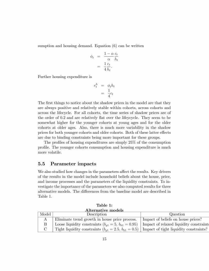
We also studied how changes in the parameters a¤ect the results. Key driversof the results in the model include household beliefs about the house, price,and income processes and the parameters of the liquidity constraints. To in-vestigate the importance of the parameters we also computed results for threealternative models. The di¤erences from the baseline model are described inTable 1.
Table 1:Alternative models
Model Description QuestionA Eliminate trend growth in house price process. Impact of beliefs on house prices?B Loose liquidity constraints (by1 = 5; bh1 = 0:95) Impact of relaxed liquidity constraints?C Tight liquidity constraints (by1 = 2:5; bh1 = 0:5) Impact of tight liquidity constraints?
15
In Model A, we eliminate the trend growth rate in housing prices. Thisresults in signi�cantly lower values of expected house price growth. There stillis some expected house price growth because the house price is an exponentialfunction of a shock. We report results of this experiment for the 1940 Cohort,High Education group. Results of this experiment are summarised in Figures45 and 46. These can be compared with the baseline results for this group inFigures 31 and 32. As one would expect, the growth in wealth in this modelis much smaller. Also, cross-sectional variability in wealth is much smaller.Also housing consumption in the low growth model is roughly half as largeas housing consumption in the baseline model. In terms of welfare, utility ishigher in the high expected house price growth world.In Model B, we investigate the impact of relaxed liquidity constraints.
A summary of these results is shown in Figures 47 and 48. With relaxedconstraints, household wealth grows much more quickly. The median levelreaches £ 150,000 by model period 32 versus £ 110,000 in the baseline model.After that, median and 90% quantile wealth levels remain higher throughoutlife. Much of this increased wealth is supported by larger investment inhousing than the baseline model and in turn supports a higher consumptionlevel than the baseline model. Also, the cross sectional variation in housingconsumption is much larger in Model B than in the baseline model. Figure 50displays the impact on utility and on the shadow price. Utility is signi�cantlyhigher in the model with relaxed constraints as one would expect. Thisdi¤erence diminishes near the end of life. Also the cross-sectional variationof utility is higher than the baseline model. For the shadow price, the shadowprice is somewhat lower at young ages. But then the 90% quantile increasesdramatically at older ages as the fraction who are constrained increases.Results from Model C are displayed in Figures 49 and 50. The di¤erences
from the baseline model are less stark but are visible. Average investment inhousing is higher in model C at younger ages. Larger quantities are requiredto borrow than in the baseline model. The cross-sectional variation in housingconsumption is also larger at young ages. Those who are more constrained arelikely to invest more in housing in order to borrow. The impact on utilityis unclear. Everything else equal, tight constraints cannot increase ex antutility however, could lead to ex post higher utility is household behaviouris forced to be more conservative.
16
6 Conclusion
In this paper we calibrate a lifecycle model of demand for housing. Themodel has stochastic house prices, interest rates, and incomes along withconstraints on borrowing that depend on household income and on the housevalue. The model is calibrated to parameters from the literature and todata from the UK FES/EFS. We use the model to study how demand forhousing and consumption as well as the welfare depend on wealth, houseprices, interest rates, income, age and birth cohort. We also use the modelto estimate shadow prices for housing.We �nd that house prices (excluding endowment income e¤ects) have
small impacts on consumption but that wealth impacts on consumption aresigni�cant. Both house price impacts and wealth impacts on housing demandare signi�cant. The shadow price of housing is an increasing function of houseprices. The impact is stronger when wealth is low.We also simulate lifecycle pro�les for 18 groups, 9 cohorts and 2 educa-
tion groups per cohort. The model produces reasonable lifecycle pro�les ofconsumption and housing demand.We �nd that reduced expectations about house price growth reduce in-
vestment in housing and reduce the rate of wealth accumulation. We also�nd that either tightening or loosening liquidity constraints have impacts onhousing, wealth and utility as one would expect.Much work remains to be done to improve the modeling approach. First,
more work can be done to �t the model to data. Our work in this dimen-sion was limited by data quality and computational considerations. Sec-ond, further investigations about alternative assumptions about the stochas-tic processes driving the model are required. Finally, several features ofthe housing market can be added to the model including transaction costs,taxes, depreciation and maintenance, choice of rental vs. ownership., andalternative assumptions about credit market conditions. These features canbe incorporated in the present model and o¤er several promising avenues forfuture work.
17

A Tables
Table A.1:Summary of notation
Variable Descriptionwt total wealth at tht quantity of housing at tct quantity of other consumption at tst bank savings (or borrowing) at tpt price of housing at trt gross interest rate at tyt income at tqt vector of (pt; rt; yt)wLt minimum feasible wealth level (see section 10 on bankruptcy)
18
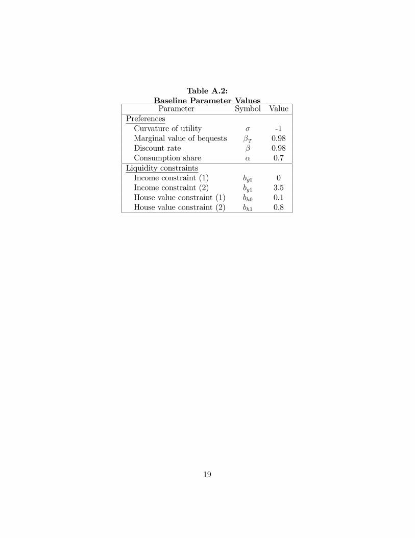
Table A.2:Baseline Parameter ValuesParameter Symbol Value
PreferencesCurvature of utility � -1Marginal value of bequests �T 0.98Discount rate � 0.98Consumption share � 0.7
Liquidity constraintsIncome constraint (1) by0 0Income constraint (2) by1 3.5House value constraint (1) bh0 0.1House value constraint (2) bh1 0.8
19
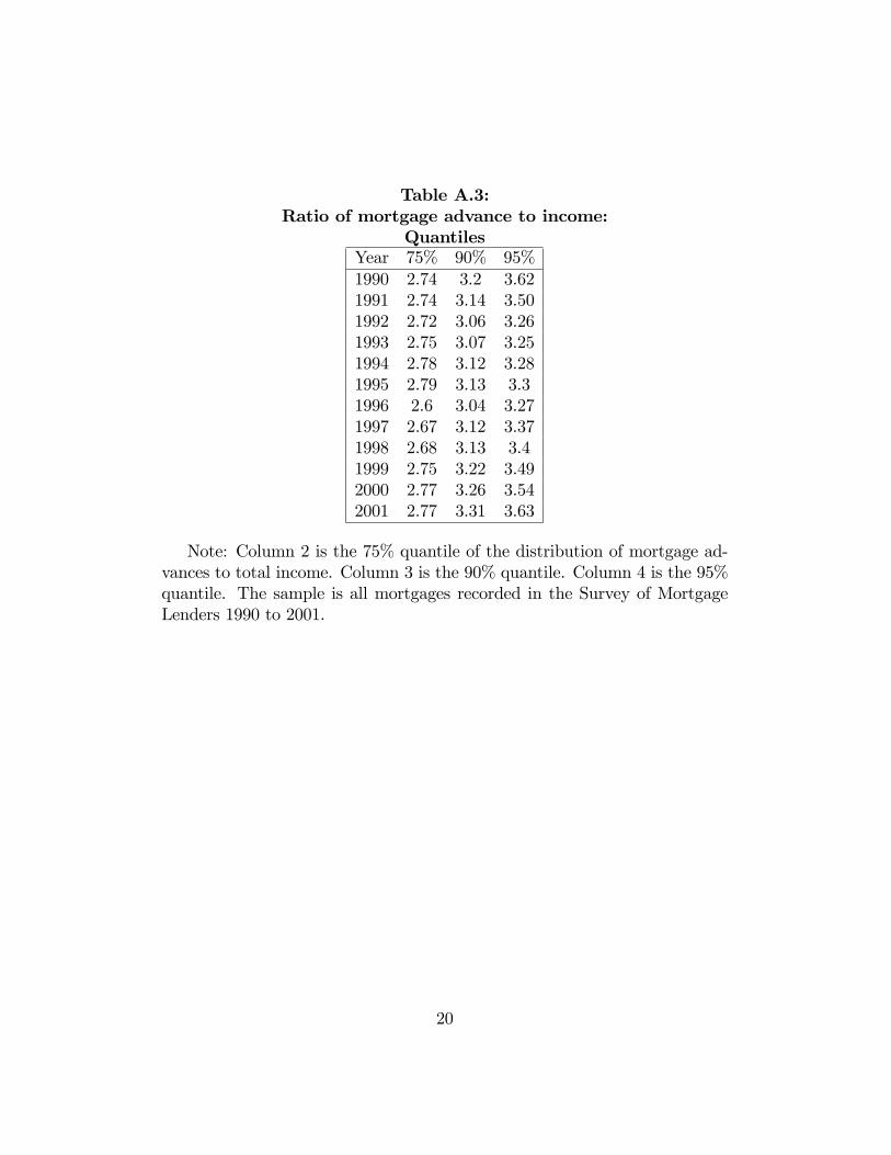
Table A.3:Ratio of mortgage advance to income:
QuantilesYear 75% 90% 95%1990 2.74 3.2 3.621991 2.74 3.14 3.501992 2.72 3.06 3.261993 2.75 3.07 3.251994 2.78 3.12 3.281995 2.79 3.13 3.31996 2.6 3.04 3.271997 2.67 3.12 3.371998 2.68 3.13 3.41999 2.75 3.22 3.492000 2.77 3.26 3.542001 2.77 3.31 3.63
Note: Column 2 is the 75% quantile of the distribution of mortgage ad-vances to total income. Column 3 is the 90% quantile. Column 4 is the 95%quantile. The sample is all mortgages recorded in the Survey of MortgageLenders 1990 to 2001.
20
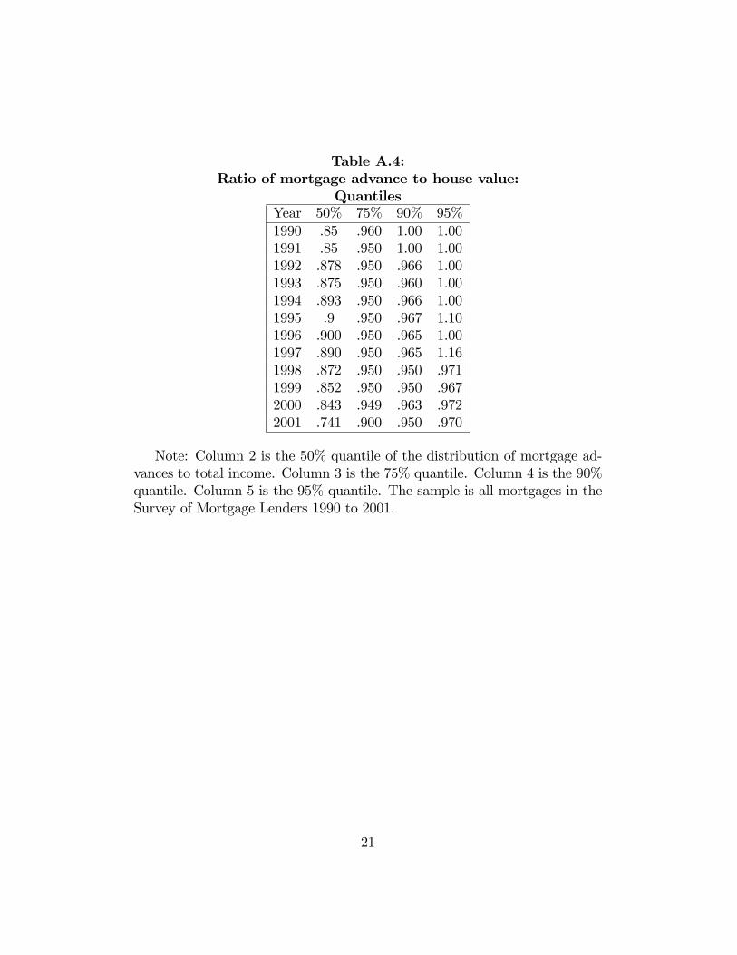
Table A.4:Ratio of mortgage advance to house value:
QuantilesYear 50% 75% 90% 95%1990 .85 .960 1.00 1.001991 .85 .950 1.00 1.001992 .878 .950 .966 1.001993 .875 .950 .960 1.001994 .893 .950 .966 1.001995 .9 .950 .967 1.101996 .900 .950 .965 1.001997 .890 .950 .965 1.161998 .872 .950 .950 .9711999 .852 .950 .950 .9672000 .843 .949 .963 .9722001 .741 .900 .950 .970
Note: Column 2 is the 50% quantile of the distribution of mortgage ad-vances to total income. Column 3 is the 75% quantile. Column 4 is the 90%quantile. Column 5 is the 95% quantile. The sample is all mortgages in theSurvey of Mortgage Lenders 1990 to 2001.
21
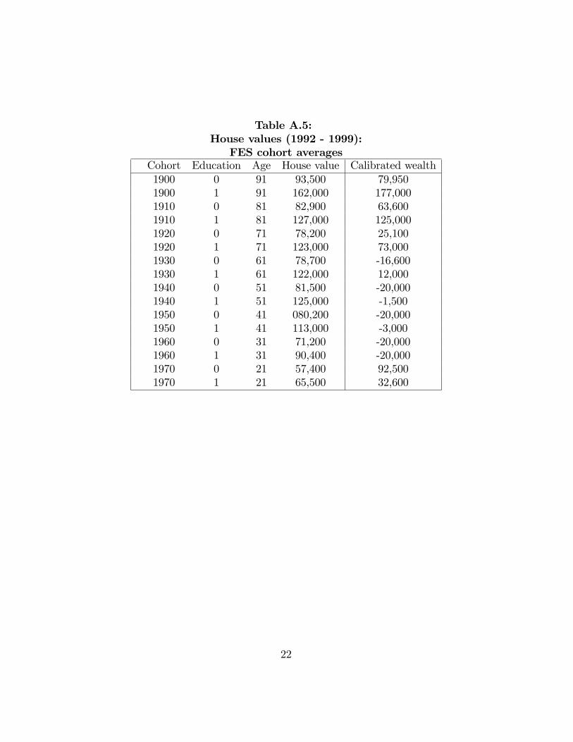
Table A.5:House values (1992 - 1999):
FES cohort averagesCohort Education Age House value Calibrated wealth1900 0 91 93,500 79,9501900 1 91 162,000 177,0001910 0 81 82,900 63,6001910 1 81 127,000 125,0001920 0 71 78,200 25,1001920 1 71 123,000 73,0001930 0 61 78,700 -16,6001930 1 61 122,000 12,0001940 0 51 81,500 -20,0001940 1 51 125,000 -1,5001950 0 41 080,200 -20,0001950 1 41 113,000 -3,0001960 0 31 71,200 -20,0001960 1 31 90,400 -20,0001970 0 21 57,400 92,5001970 1 21 65,500 32,600
22
B Computation
Let V (wt; qt; t) be the value function for a household in period t with wealthwt facing prices qt where qt = (pt; rt; yt) :6 That is, V measures the maximumlevel of utility or welfare obtainable by a household when wealth is w andprices are q in period t: Further let c (wt; qt; t) ; s (wt; qt; t) ; and h (wt; qt; t)be the optimal policy functions of such a household. These describe optimalchoices of consumption, savings, and housing as functions of wealth, prices,and time.Our computational methods compute numerical approximations to these
four functions. Because the approximation technique for each of the fourfunctions is similar. We only detail approximation of the value function V:We will approximate V with the function
bV (w; q; t) = JXj=1
aj (t)�j (w; q)
where the functions �j (w; q) j = 1; :::; J are suitably chosen basis functions(tensor products of univariate spline functions) and the coe¢ cients aj (t)j = 1; :::; J are computed by solving the problem
minfag
8<:NXi=1
!i
"V (wi; qi; t)�
JXj=1
aj (t)�j (wi; qi)
#29=; (10)
where f!igNi=1 are appropriately chosen weights.The following algorithm is used to compute these approximations.
1. Fix a grid (wi; qi) for i = 1; :::; N: Each point in this grid is an elementof R4:
2. Fix a set of basis functions �j (w; q) for j = 1; :::; J:
3. Set t = T:
4. For each i; set wT = wi and qT = qi and compute the solution to thehousehold�s period T problem: The result is a set of values for the valuefunction V (wi; qi; T ) :
6When there are no �xed costs, the value function does not depend on h explicitly.
23
5. Compute the coe¢ cients aj (T ) that solve problem (10) :
6. Set t = T � 1:
7. For each i; set wT�1 = wi and qT�1 = qi and compute the solution to thehousehold�s period T �1 problem with bV (w; q; T ) replacing V (w; q; T )and with the integral computed by Gaussian quadrature techniques.The result is a set of values for the value function V (wi; qi; T � 1) :
8. Compute the coe¢ cients aj (T � 1) that solve problem (10) :
This process is repeated for each period. In practice, values for the policyfunctions are saved as well and the actual grid chosen varies with each period.Additionally, our baseline model requires us to approximate a three di-
mensional integral. We approximate this using Gaussian quadrature. Ex-tensions to the baseline model require approximation of a six dimensionalintegral. Again we will use Gaussian quadrature to approximate these inte-grals.Compute code for this model is published can be found at
24
References
[1] Attanasio, O., Blow, L., Hamilton, R., and A. Leicester (2004), �Boomsand Busts: Consumption, House Prices and Expectations,� Bank ofEngland Working Paper.
[2] Attanasio, O. and Weber, G. (1994), �The UK Consumption Boom ofthe Late 1980�s: Aggregate Implications of Microeconomic Evidence,"The Economic Journal, 104(427): 1269-1302.
[3] Banks, J., Blundell, R., Smith, J., and Z. Smith (2004), �House PriceVolatility and Housing Ownership over the Lifecycle,�University CollegeLondon, Department of Economics Discussion Paper 04-09.
[4] Blundell, R., Browning, M. and C. Meghir (1994), �Consumer Demandand the Life-Cycle Allocation of Household Expenditure�, Review ofEconomic Studies, 61, 57-80.
[5] Campbell, John and Cocco, João (2007), �How Do House Prices A¤ectConsumption: Evidence from Microdata," Journal of Monetary Eco-nomics, 54: 591-621.
[6] Crawford, I. (1994), �UK household cost-of-living indices, 1979-1992�,Institute for Fiscal Studies Commentary C44.
[7] Deaton, A. (1991), �Saving and Liquidity Constraints�, Econometrica,59(5): 1221-1248.
[8] Díaz, Antonia, and Luengo-Prado, María José (2007), �On the User Costand Homeownership," Review of Economic Dynamics, 11: 584-613.
[9] Disney, R., Henley, A. and Jevons, D. (2003) �House price shocks, neg-ative equity and household consumption in the UK�, mimeo, Universityof Nottingham.
[10] Fernandez-Villaverde, J. and D. Krueger (2001), �Consumption andSaving over the Life Cycle: How Important are Consumer Durables?�,mimeo.
[11] Goodman, A. and Old�eld, Z. (2004) �Permanent di¤erences? Incomeand expenditure inequality in the 1990s and 2000s�, IFS Reports, R66.
25
[12] Judd, K. (1998), Numerical Methods in Economics, The MIT Press:Cambridge.
[13] Li, Wenli and Yao, Rui (2007), �The Life-Cycle E¤ects of House PriceChanges," Journal of Money, Credit and Banking, 39(6): 1375-1409.
[14] Muellbauer, J. and A. Murphy (1997), �Booms and Busts in the UKHousing Market,�The Economic Journal, 107(445): 1701-1727.
[15] Nesheim, Lars. and Skrainka, Ben (2009), "Fortran Code to Simulatea Lifecycle Housing Model," CEMMAP Software CS2009/01, http://cemmap.ac.uk.
[16] Poterba, J. (1992), �Taxation and Housing: Old Questions, New An-swers,�The American Economic Review, 82(2): 237-242.
[17] Robinson, B. and Skinner, T. (1989), �Reforming the RPI: a bettertreatment of housing costs".
26
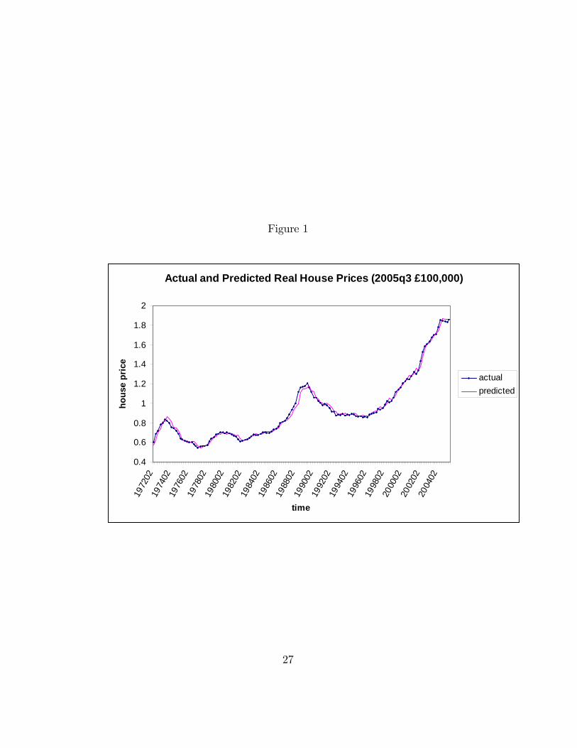
Figure 1
Actual and Predicted Real House Prices (2005q3 £100,000)
0.4
0.6
0.8
1
1.2
1.4
1.6
1.8
2
1972
0219
7402
1976
0219
7802
1980
0219
8202
1984
0219
8602
1988
0219
9002
1992
0219
9402
1996
0219
9802
2000
0220
0202
2004
02
time
hous
e pr
ice
actualpredicted
27
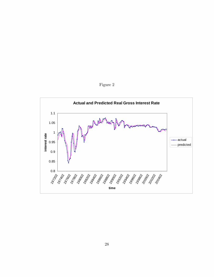
Figure 2
Actual and Predicted Real Gross Interest Rate
0.8
0.85
0.9
0.95
1
1.05
1.1
1972
0219
7402
1976
0219
7802
1980
0219
8202
1984
0219
8602
1988
0219
9002
1992
0219
9402
1996
0219
9802
2000
0220
0202
2004
02
time
inte
rest
rate
actualpredicted
28
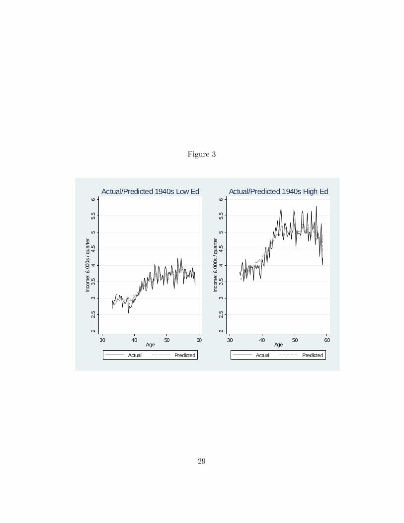
Figure 3
22.
53
3.5
44.
55
5.5
6In
com
e: £
000
s / q
uarte
r
30 40 50 60Age
Actual Predicted
Actual/Predicted 1940s Low Ed
22.
53
3.5
44.
55
5.5
6In
com
e: £
000
s / q
uarte
r
30 40 50 60Age
Actual Predicted
Actual/Predicted 1940s High Ed
29
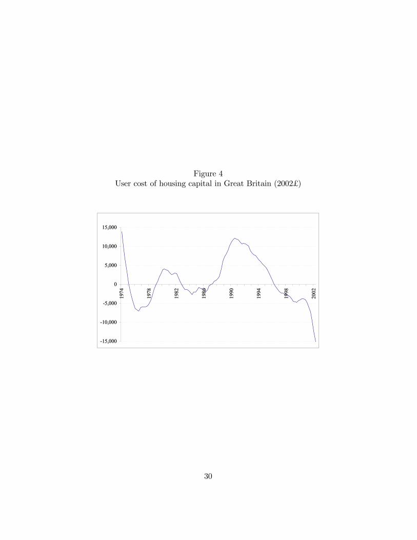
Figure 4User cost of housing capital in Great Britain (2002£ )
30
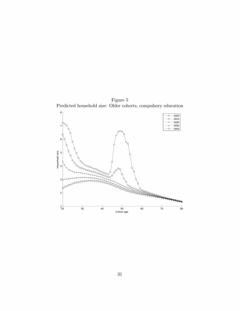
Figure 5Predicted household size: Older cohorts, compulsory education
20 30 40 50 60 70 801
2
3
4
5
6
7
8
Cohort age
Hou
seho
ld s
ize
19001910192019301940
31
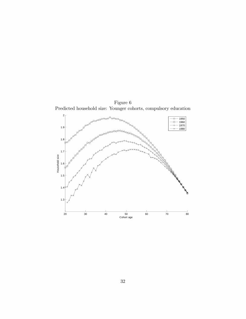
Figure 6Predicted household size: Younger cohorts, compulsory education
20 30 40 50 60 70 80
1.3
1.4
1.5
1.6
1.7
1.8
1.9
2
Cohort age
Hou
seho
ld s
ize
1950196019701980
32
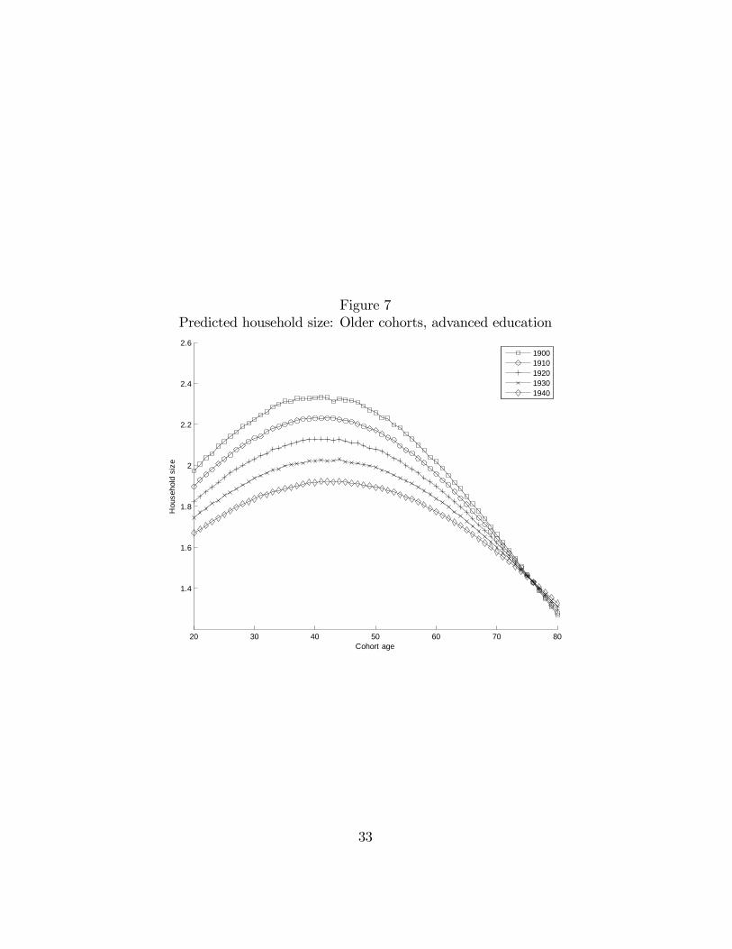
Figure 7Predicted household size: Older cohorts, advanced education
20 30 40 50 60 70 80
1.4
1.6
1.8
2
2.2
2.4
2.6
Cohort age
Hou
seho
ld s
ize
19001910192019301940
33
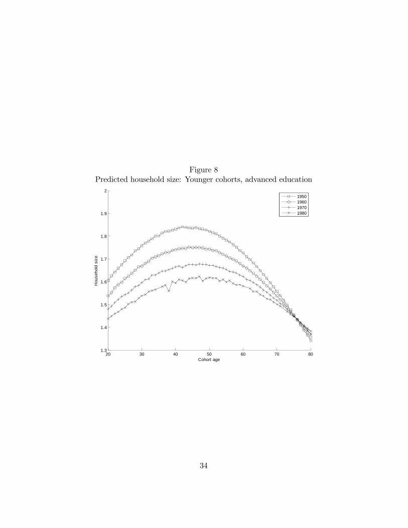
Figure 8Predicted household size: Younger cohorts, advanced education
20 30 40 50 60 70 801.3
1.4
1.5
1.6
1.7
1.8
1.9
2
Cohort age
Hou
seho
ld s
ize
1950196019701980
34
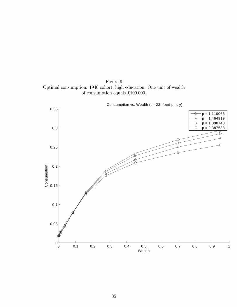
Figure 9Optimal consumption: 1940 cohort, high education. One unit of wealth
of consumption equals £ 100,000.
0 0.1 0.2 0.3 0.4 0.5 0.6 0.7 0.8 0.9 10
0.05
0.1
0.15
0.2
0.25
0.3
0.35
Wealth
Con
sum
ptio
n
Consumption vs. Wealth (t = 23; fixed p, r, y)
p = 1.110066p = 1.464919p = 1.890743p = 2.387538
35
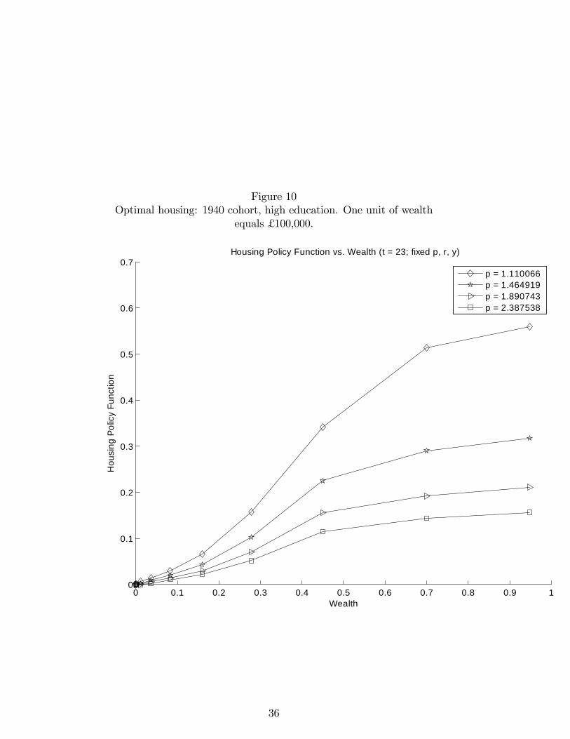
Figure 10Optimal housing: 1940 cohort, high education. One unit of wealth
equals £ 100,000.
0 0.1 0.2 0.3 0.4 0.5 0.6 0.7 0.8 0.9 10
0.1
0.2
0.3
0.4
0.5
0.6
0.7
Wealth
Hou
sing
Pol
icy
Func
tion
Housing Policy Function vs. Wealth (t = 23; fixed p, r, y)
p = 1.110066p = 1.464919p = 1.890743p = 2.387538
36
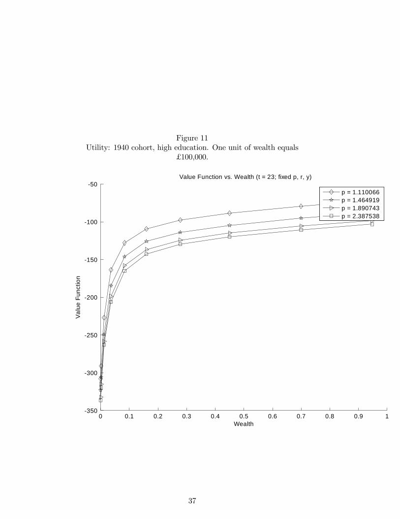
Figure 11Utility: 1940 cohort, high education. One unit of wealth equals
£ 100,000.
0 0.1 0.2 0.3 0.4 0.5 0.6 0.7 0.8 0.9 1350
300
250
200
150
100
50
Wealth
Valu
e Fu
nctio
n
Value Function vs. Wealth (t = 23; fixed p, r, y)
p = 1.110066p = 1.464919p = 1.890743p = 2.387538
37
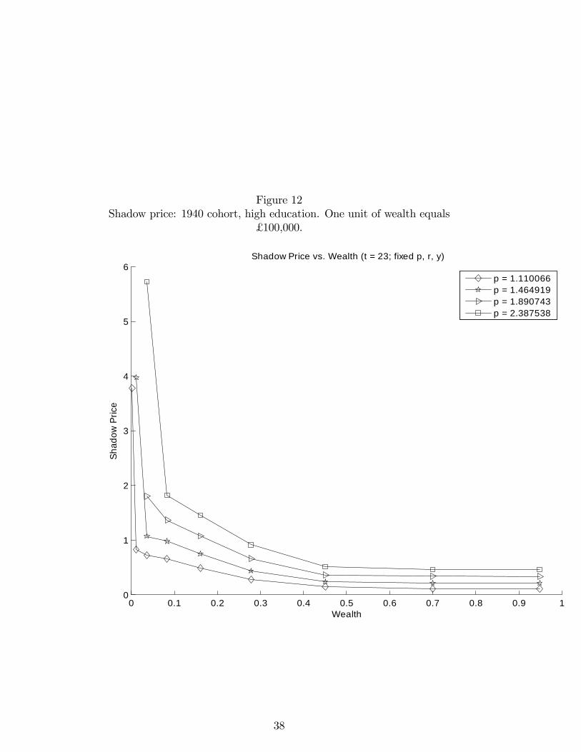
Figure 12Shadow price: 1940 cohort, high education. One unit of wealth equals
£ 100,000.
0 0.1 0.2 0.3 0.4 0.5 0.6 0.7 0.8 0.9 10
1
2
3
4
5
6
Wealth
Shad
ow P
rice
Shadow Price vs. Wealth (t = 23; fixed p, r, y)
p = 1.110066p = 1.464919p = 1.890743p = 2.387538
38

Figure 13Wealth, housing and consumption: 1900 Cohort, Low Education
66 68 70 72 74 76 78 80 82 840
0.5
1
1.5
T ime Period
Wea
lth
mean10th Quantile50th Quantile90th Quantile
66 68 70 72 74 76 78 80 82 840
0.5
1
1.5
T ime Period
Hou
sing
mean10th Quantile50th Quantile90th Quantile
66 68 70 72 74 76 78 80 82 840
0.1
0.2
0.3
0.4
T ime Period
Con
sum
ptio
n mean10th Quantile50th Quantile90th Quantile
Figure 14Utility and the shadow price: 1900 Cohort, Low Education
66 68 70 72 74 76 78 80 82 8480
60
40
20
0
20
T ime Period
Val
ue F
unct
ion
mean10th Quantile50th Quantile90th Quantile
66 68 70 72 74 76 78 80 82 840
0.1
0.2
0.3
0.4
0.5
T ime Period
Sha
dow
Pric
e
mean10th Quantile50th Quantile90th Quantile
39
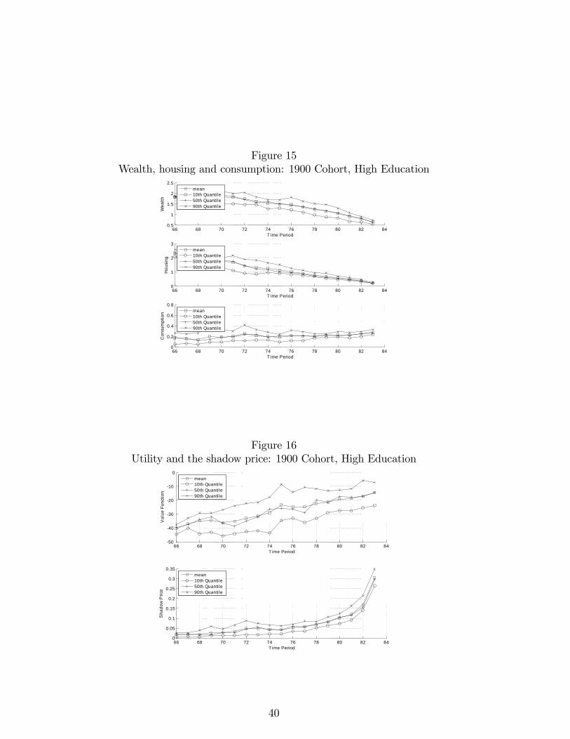
Figure 15Wealth, housing and consumption: 1900 Cohort, High Education
66 68 70 72 74 76 78 80 82 840.5
1
1.5
2
2.5
T ime Period
Wea
lth
mean10th Quantile50th Quantile90th Quantile
66 68 70 72 74 76 78 80 82 840
1
2
3
T ime Period
Hou
sing
mean10th Quantile50th Quantile90th Quantile
66 68 70 72 74 76 78 80 82 840
0.2
0.4
0.6
0.8
T ime Period
Con
sum
ptio
n mean10th Quantile50th Quantile90th Quantile
Figure 16Utility and the shadow price: 1900 Cohort, High Education
66 68 70 72 74 76 78 80 82 8450
40
30
20
10
0
T ime Period
Val
ue F
unct
ion
mean10th Quanti le50th Quanti le90th Quanti le
66 68 70 72 74 76 78 80 82 840
0.05
0.1
0.15
0.2
0.25
0.3
0.35
T ime Period
Sha
dow
Pric
e
mean10th Quanti le50th Quanti le90th Quanti le
40
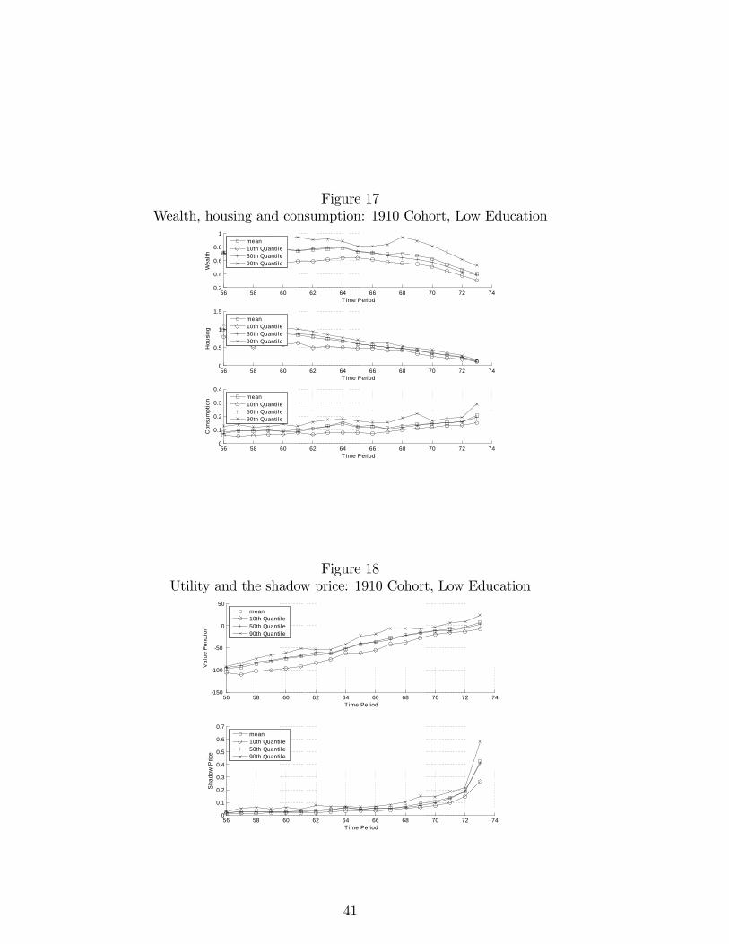
Figure 17Wealth, housing and consumption: 1910 Cohort, Low Education
56 58 60 62 64 66 68 70 72 740.2
0.4
0.6
0.8
1
T ime Period
Wea
lth
mean10th Quantile50th Quantile90th Quantile
56 58 60 62 64 66 68 70 72 740
0.5
1
1.5
T ime Period
Hou
sing
mean10th Quantile50th Quantile90th Quantile
56 58 60 62 64 66 68 70 72 740
0.1
0.2
0.3
0.4
T ime Period
Con
sum
ptio
n mean10th Quantile50th Quantile90th Quantile
Figure 18Utility and the shadow price: 1910 Cohort, Low Education
56 58 60 62 64 66 68 70 72 74150
100
50
0
50
T ime Period
Val
ue F
unct
ion
mean10th Quantile50th Quantile90th Quantile
56 58 60 62 64 66 68 70 72 740
0.1
0.2
0.3
0.4
0.5
0.6
0.7
T ime Period
Sha
dow
Pric
e
mean10th Quantile50th Quantile90th Quantile
41
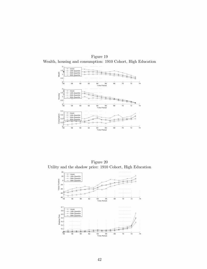
Figure 19Wealth, housing and consumption: 1910 Cohort, High Education
56 58 60 62 64 66 68 70 72 740
0.5
1
1.5
2
T ime Period
Wea
lth
mean10th Quantile50th Quantile90th Quantile
56 58 60 62 64 66 68 70 72 740
0.5
1
1.5
2
T ime Period
Hou
sing
mean10th Quantile50th Quantile90th Quantile
56 58 60 62 64 66 68 70 72 740
0.1
0.2
0.3
0.4
T ime Period
Con
sum
ptio
n mean10th Quantile50th Quantile90th Quantile
Figure 20Utility and the shadow price: 1910 Cohort, High Education
56 58 60 62 64 66 68 70 72 7480
60
40
20
0
20
40
T ime Period
Val
ue F
unct
ion
mean10th Quantile50th Quantile90th Quantile
56 58 60 62 64 66 68 70 72 740
0.1
0.2
0.3
0.4
0.5
0.6
0.7
T ime Period
Sha
dow
Pric
e
mean10th Quantile50th Quantile90th Quantile
42
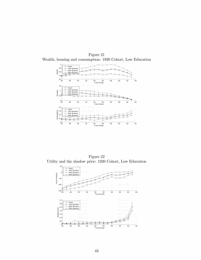
Figure 21Wealth, housing and consumption: 1920 Cohort, Low Education
46 48 50 52 54 56 58 60 62 640.2
0.4
0.6
0.8
1
T ime Period
Wea
lth
mean10th Quantile50th Quantile90th Quantile
46 48 50 52 54 56 58 60 62 640
0.5
1
1.5
T ime Period
Hou
sing
mean10th Quantile50th Quantile90th Quantile
46 48 50 52 54 56 58 60 62 640
0.1
0.2
0.3
0.4
T ime Period
Con
sum
ptio
n mean10th Quantile50th Quantile90th Quantile
Figure 22Utility and the shadow price: 1920 Cohort, Low Education
46 48 50 52 54 56 58 60 62 64150
100
50
0
50
T ime Period
Val
ue F
unct
ion
mean10th Quantile50th Quantile90th Quantile
46 48 50 52 54 56 58 60 62 640
0.1
0.2
0.3
0.4
0.5
0.6
0.7
T ime Period
Sha
dow
Pric
e
mean10th Quantile50th Quantile90th Quantile
43
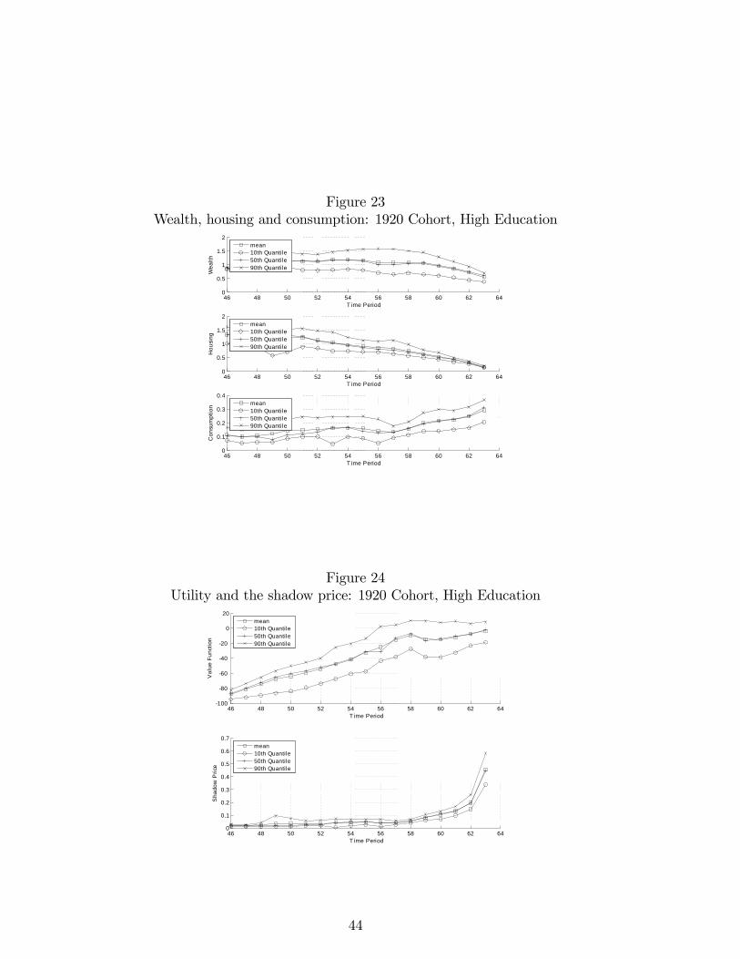
Figure 23Wealth, housing and consumption: 1920 Cohort, High Education
46 48 50 52 54 56 58 60 62 640
0.5
1
1.5
2
T ime Period
Wea
lth
mean10th Quantile50th Quantile90th Quantile
46 48 50 52 54 56 58 60 62 640
0.5
1
1.5
2
T ime Period
Hou
sing
mean10th Quantile50th Quantile90th Quantile
46 48 50 52 54 56 58 60 62 640
0.1
0.2
0.3
0.4
T ime Period
Con
sum
ptio
n mean10th Quantile50th Quantile90th Quantile
Figure 24Utility and the shadow price: 1920 Cohort, High Education
46 48 50 52 54 56 58 60 62 64100
80
60
40
20
0
20
Time Period
Val
ue F
unct
ion
mean10th Quantile50th Quantile90th Quantile
46 48 50 52 54 56 58 60 62 640
0.1
0.2
0.3
0.4
0.5
0.6
0.7
T ime Period
Sha
dow
Pric
e
mean10th Quantile50th Quantile90th Quantile
44
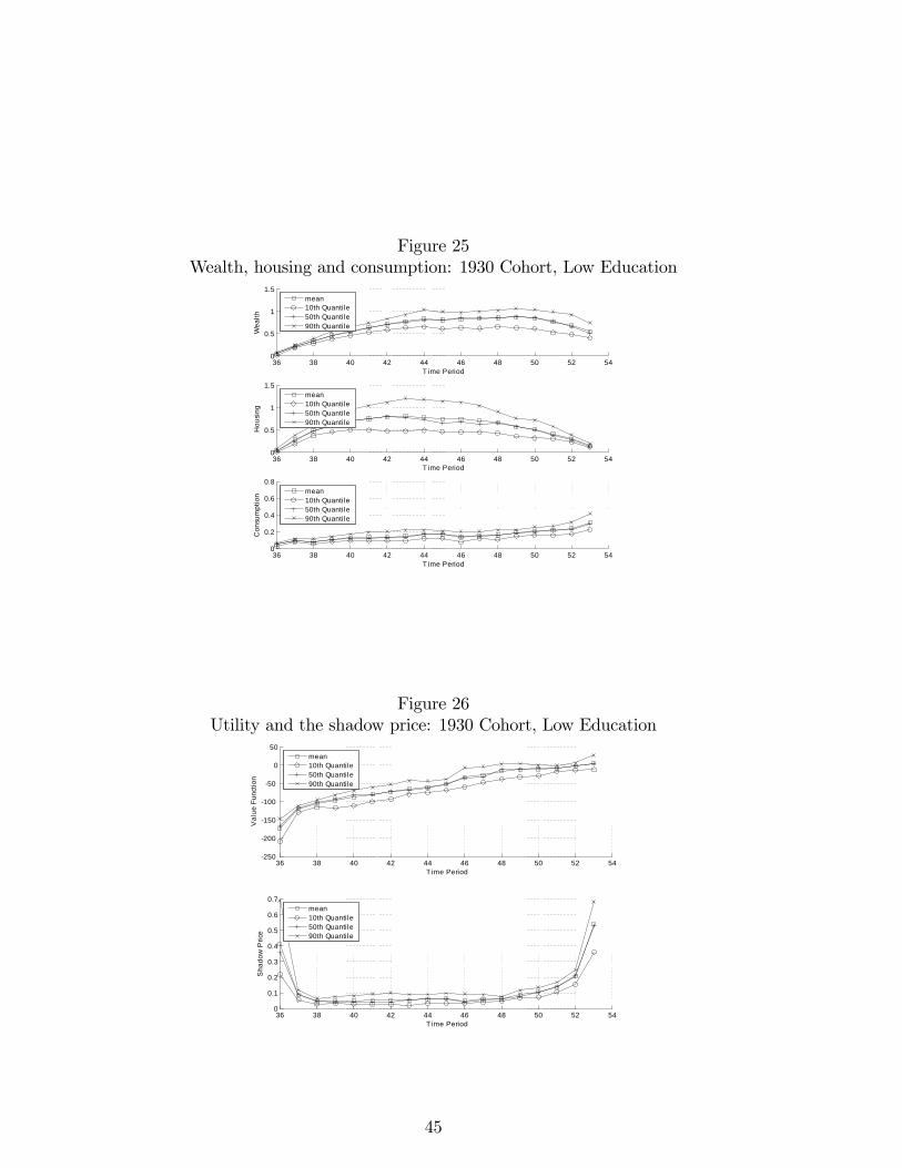
Figure 25Wealth, housing and consumption: 1930 Cohort, Low Education
36 38 40 42 44 46 48 50 52 540
0.5
1
1.5
T ime Period
Wea
lth
mean10th Quantile50th Quantile90th Quantile
36 38 40 42 44 46 48 50 52 540
0.5
1
1.5
T ime Period
Hou
sing
mean10th Quantile50th Quantile90th Quantile
36 38 40 42 44 46 48 50 52 540
0.2
0.4
0.6
0.8
T ime Period
Con
sum
ptio
n mean10th Quantile50th Quantile90th Quantile
Figure 26Utility and the shadow price: 1930 Cohort, Low Education
36 38 40 42 44 46 48 50 52 54250
200
150
100
50
0
50
T ime Period
Val
ue F
unct
ion
mean10th Quantile50th Quantile90th Quantile
36 38 40 42 44 46 48 50 52 540
0.1
0.2
0.3
0.4
0.5
0.6
0.7
T ime Period
Sha
dow
Pric
e
mean10th Quantile50th Quantile90th Quantile
45
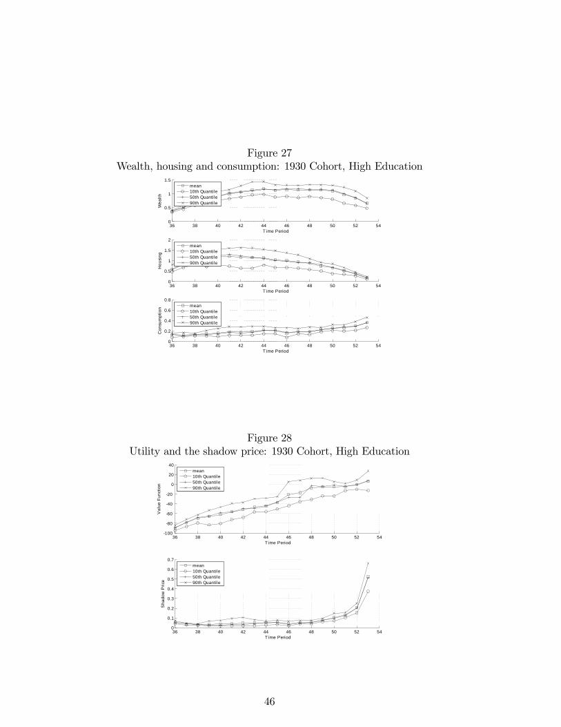
Figure 27Wealth, housing and consumption: 1930 Cohort, High Education
36 38 40 42 44 46 48 50 52 540
0.5
1
1.5
T ime Period
Wea
lth
mean10th Quantile50th Quantile90th Quantile
36 38 40 42 44 46 48 50 52 540
0.5
1
1.5
2
T ime Period
Hou
sing
mean10th Quantile50th Quantile90th Quantile
36 38 40 42 44 46 48 50 52 540
0.2
0.4
0.6
0.8
T ime Period
Con
sum
ptio
n mean10th Quantile50th Quantile90th Quantile
Figure 28Utility and the shadow price: 1930 Cohort, High Education
36 38 40 42 44 46 48 50 52 54100
80
60
40
20
0
20
40
Time Period
Val
ue F
unct
ion
mean10th Quantile50th Quantile90th Quantile
36 38 40 42 44 46 48 50 52 540
0.1
0.2
0.3
0.4
0.5
0.6
0.7
T ime Period
Sha
dow
Pric
e
mean10th Quantile50th Quantile90th Quantile
46
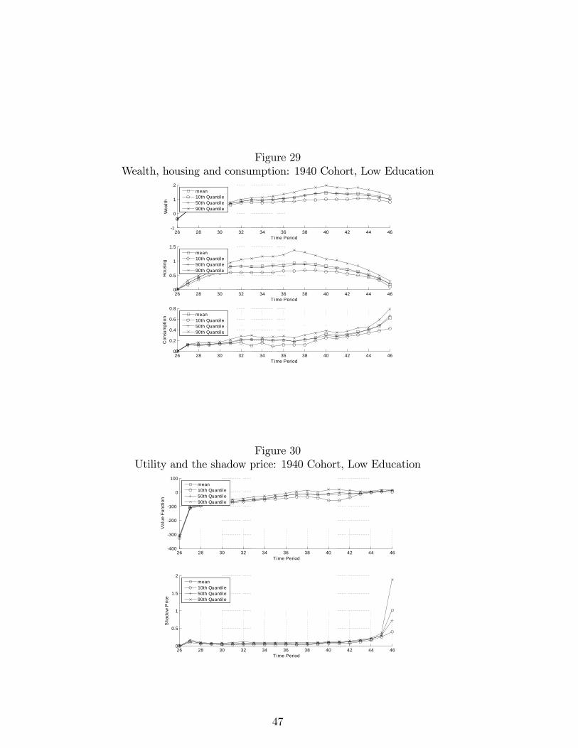
Figure 29Wealth, housing and consumption: 1940 Cohort, Low Education
26 28 30 32 34 36 38 40 42 44 461
0
1
2
T ime Period
Wea
lth
mean10th Quantile50th Quantile90th Quantile
26 28 30 32 34 36 38 40 42 44 460
0.5
1
1.5
T ime Period
Hou
sing
mean10th Quantile50th Quantile90th Quantile
26 28 30 32 34 36 38 40 42 44 460
0.2
0.4
0.6
0.8
T ime Period
Con
sum
ptio
n mean10th Quantile50th Quantile90th Quantile
Figure 30Utility and the shadow price: 1940 Cohort, Low Education
26 28 30 32 34 36 38 40 42 44 46400
300
200
100
0
100
T ime Period
Val
ue F
unct
ion
mean10th Quantile50th Quantile90th Quantile
26 28 30 32 34 36 38 40 42 44 460
0.5
1
1.5
2
T ime Period
Sha
dow
Pric
e
mean10th Quantile50th Quantile90th Quantile
47
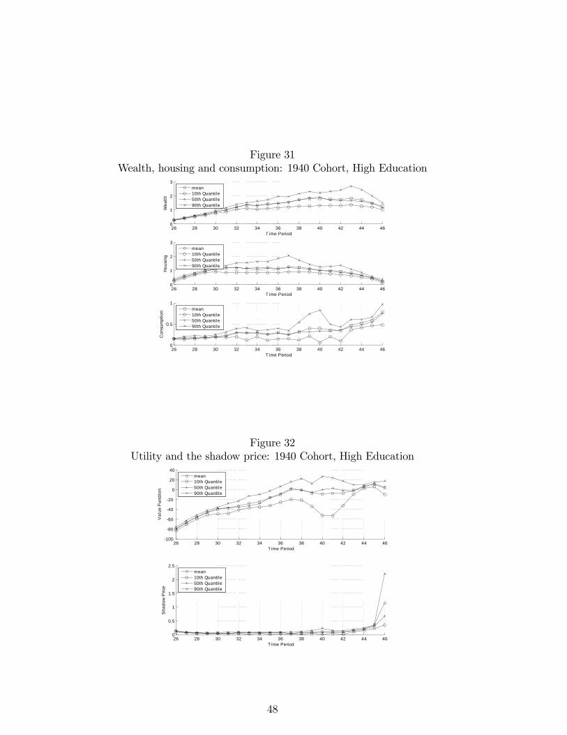
Figure 31Wealth, housing and consumption: 1940 Cohort, High Education
26 28 30 32 34 36 38 40 42 44 460
1
2
3
T ime Period
Wea
lth
mean10th Quantile50th Quantile90th Quantile
26 28 30 32 34 36 38 40 42 44 460
1
2
3
T ime Period
Hou
sing
mean10th Quantile50th Quantile90th Quantile
26 28 30 32 34 36 38 40 42 44 460
0.5
1
T ime Period
Con
sum
ptio
n mean10th Quantile50th Quantile90th Quantile
Figure 32Utility and the shadow price: 1940 Cohort, High Education
26 28 30 32 34 36 38 40 42 44 46100
80
60
40
20
0
20
40
T ime Period
Val
ue F
unct
ion
mean10th Quantile50th Quantile90th Quantile
26 28 30 32 34 36 38 40 42 44 460
0.5
1
1.5
2
2.5
T ime Period
Sha
dow
Pric
e
mean10th Quantile50th Quantile90th Quantile
48
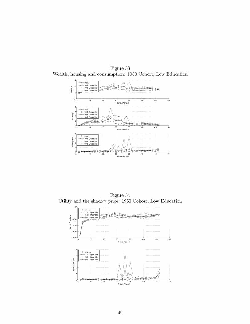
Figure 33Wealth, housing and consumption: 1950 Cohort, Low Education
15 20 25 30 35 40 45 502
0
2
4
T ime Period
Wea
lth
mean10th Quantile50th Quantile90th Quantile
15 20 25 30 35 40 45 500
1
2
3
4
T ime Period
Hou
sing
mean10th Quantile50th Quantile90th Quantile
15 20 25 30 35 40 45 500
1
2
3
4
T ime Period
Con
sum
ptio
n mean10th Quantile50th Quantile90th Quantile
Figure 34Utility and the shadow price: 1950 Cohort, Low Education
15 20 25 30 35 40 45 50400
300
200
100
0
100
T ime Period
Val
ue F
unct
ion
mean10th Quantile50th Quantile90th Quantile
15 20 25 30 35 40 45 500
1
2
3
4
5
T ime Period
Sha
dow
Pric
e
mean10th Quantile50th Quantile90th Quantile
49
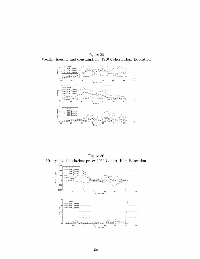
Figure 35Wealth, housing and consumption: 1950 Cohort, High Education
15 20 25 30 35 40 45 500
1
2
3
4
T ime Period
Wea
lth
mean10th Quanti le50th Quanti le90th Quanti le
15 20 25 30 35 40 45 500
1
2
3
T ime Period
Hou
sing
mean10th Quanti le50th Quanti le90th Quanti le
15 20 25 30 35 40 45 500
1
2
3
T ime Period
Con
sum
ptio
n mean10th Quanti le50th Quanti le90th Quanti le
Figure 36Utility and the shadow price: 1950 Cohort, High Education
15 20 25 30 35 40 45 501000
500
0
500
1000
1500
T ime Period
Val
ue F
unct
ion
mean10th Quantile50th Quantile90th Quantile
15 20 25 30 35 40 45 500
2
4
6
8
T ime Period
Sha
dow
Pric
e
mean10th Quantile50th Quantile90th Quantile
50
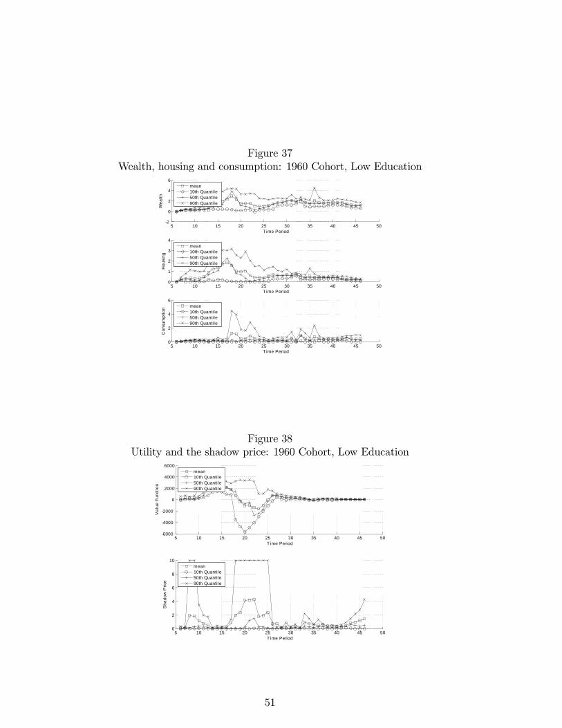
Figure 37Wealth, housing and consumption: 1960 Cohort, Low Education
5 10 15 20 25 30 35 40 45 502
0
2
4
6
T ime Period
Wea
lth
mean10th Quantile50th Quantile90th Quantile
5 10 15 20 25 30 35 40 45 500
1
2
3
4
T ime Period
Hou
sing
mean10th Quantile50th Quantile90th Quantile
5 10 15 20 25 30 35 40 45 500
2
4
6
T ime Period
Con
sum
ptio
n mean10th Quantile50th Quantile90th Quantile
Figure 38Utility and the shadow price: 1960 Cohort, Low Education
5 10 15 20 25 30 35 40 45 506000
4000
2000
0
2000
4000
6000
T ime Period
Val
ue F
unct
ion
mean10th Quantile50th Quantile90th Quantile
5 10 15 20 25 30 35 40 45 500
2
4
6
8
10
T ime Period
Sha
dow
Pric
e
mean10th Quantile50th Quantile90th Quantile
51
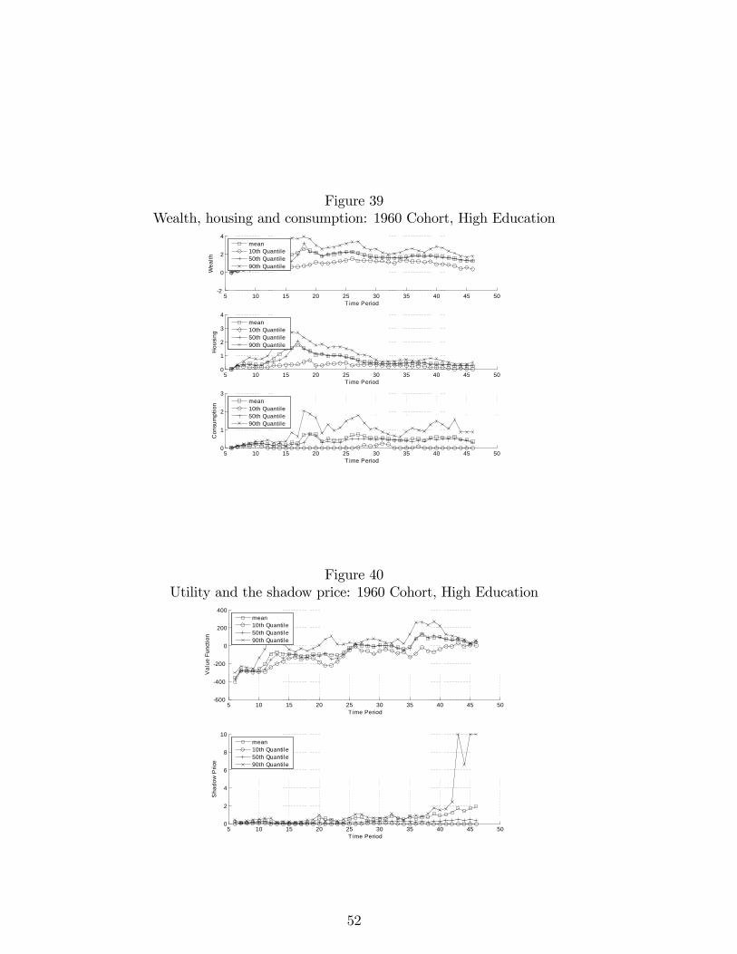
Figure 39Wealth, housing and consumption: 1960 Cohort, High Education
5 10 15 20 25 30 35 40 45 502
0
2
4
T ime Period
Wea
lth
mean10th Quantile50th Quantile90th Quantile
5 10 15 20 25 30 35 40 45 500
1
2
3
4
T ime Period
Hou
sing
mean10th Quantile50th Quantile90th Quantile
5 10 15 20 25 30 35 40 45 500
1
2
3
T ime Period
Con
sum
ptio
n mean10th Quantile50th Quantile90th Quantile
Figure 40Utility and the shadow price: 1960 Cohort, High Education
5 10 15 20 25 30 35 40 45 50600
400
200
0
200
400
T ime Period
Val
ue F
unct
ion
mean10th Quantile50th Quantile90th Quantile
5 10 15 20 25 30 35 40 45 500
2
4
6
8
10
T ime Period
Sha
dow
Pric
e
mean10th Quantile50th Quantile90th Quantile
52
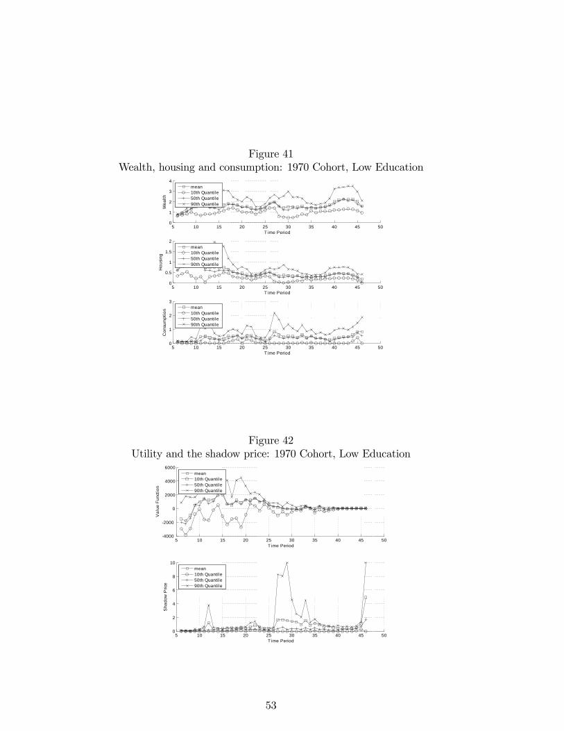
Figure 41Wealth, housing and consumption: 1970 Cohort, Low Education
5 10 15 20 25 30 35 40 45 500
1
2
3
4
T ime Period
Wea
lth
mean10th Quantile50th Quantile90th Quantile
5 10 15 20 25 30 35 40 45 500
0.5
1
1.5
2
T ime Period
Hou
sing
mean10th Quantile50th Quantile90th Quantile
5 10 15 20 25 30 35 40 45 500
1
2
3
T ime Period
Con
sum
ptio
n mean10th Quantile50th Quantile90th Quantile
Figure 42Utility and the shadow price: 1970 Cohort, Low Education
5 10 15 20 25 30 35 40 45 504000
2000
0
2000
4000
6000
T ime Period
Val
ue F
unct
ion
mean10th Quantile50th Quantile90th Quantile
5 10 15 20 25 30 35 40 45 500
2
4
6
8
10
T ime Period
Sha
dow
Pric
e
mean10th Quantile50th Quantile90th Quantile
53
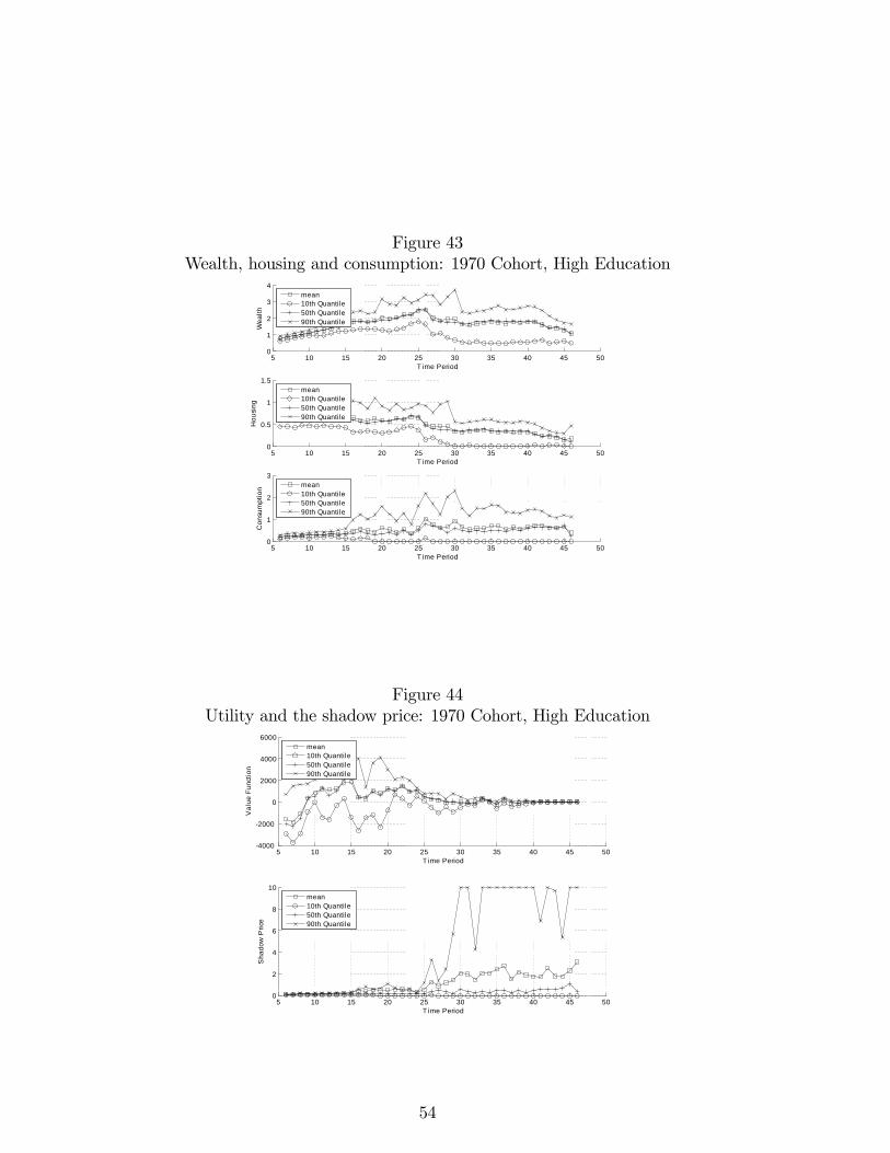
Figure 43Wealth, housing and consumption: 1970 Cohort, High Education
5 10 15 20 25 30 35 40 45 500
1
2
3
4
T ime Period
Wea
lth
mean10th Quantile50th Quantile90th Quantile
5 10 15 20 25 30 35 40 45 500
0.5
1
1.5
T ime Period
Hou
sing
mean10th Quantile50th Quantile90th Quantile
5 10 15 20 25 30 35 40 45 500
1
2
3
T ime Period
Con
sum
ptio
n mean10th Quantile50th Quantile90th Quantile
Figure 44Utility and the shadow price: 1970 Cohort, High Education
5 10 15 20 25 30 35 40 45 504000
2000
0
2000
4000
6000
T ime Period
Val
ue F
unct
ion
mean10th Quantile50th Quantile90th Quantile
5 10 15 20 25 30 35 40 45 500
2
4
6
8
10
T ime Period
Sha
dow
Pric
e
mean10th Quantile50th Quantile90th Quantile
54
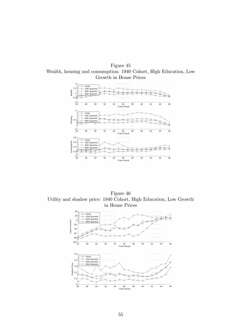
Figure 45Wealth, housing and consumption: 1940 Cohort, High Education, Low
Growth in House Prices
26 28 30 32 34 36 38 40 42 44 460
0.5
1
1.5
2
T ime Period
Wea
lth
mean10th Quantile50th Quantile90th Quantile
26 28 30 32 34 36 38 40 42 44 460
0.5
1
T ime Period
Hou
sing
mean10th Quantile50th Quantile90th Quantile
26 28 30 32 34 36 38 40 42 44 460
0.2
0.4
0.6
0.8
T ime Period
Con
sum
ptio
n mean10th Quantile50th Quantile90th Quantile
Figure 46Utility and shadow price: 1940 Cohort, High Education, Low Growth
in House Prices
26 28 30 32 34 36 38 40 42 44 46100
80
60
40
20
0
20
40
T ime Period
Val
ue F
unct
ion
mean10th Quantile50th Quantile90th Quantile
26 28 30 32 34 36 38 40 42 44 460
0.1
0.2
0.3
0.4
0.5
T ime Period
Sha
dow
Pric
e
mean10th Quantile50th Quantile90th Quantile
55
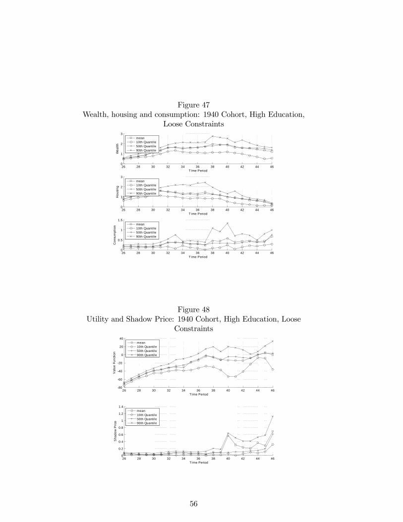
Figure 47Wealth, housing and consumption: 1940 Cohort, High Education,
Loose Constraints
26 28 30 32 34 36 38 40 42 44 460
1
2
3
T ime Period
Wea
lth
mean10th Quantile50th Quantile90th Quantile
26 28 30 32 34 36 38 40 42 44 460
1
2
3
T ime Period
Hou
sing
mean10th Quantile50th Quantile90th Quantile
26 28 30 32 34 36 38 40 42 44 460
0.5
1
1.5
T ime Period
Con
sum
ptio
n mean10th Quantile50th Quantile90th Quantile
Figure 48Utility and Shadow Price: 1940 Cohort, High Education, Loose
Constraints
26 28 30 32 34 36 38 40 42 44 4680
60
40
20
0
20
40
T ime Period
Val
ue F
unct
ion
mean10th Quantile50th Quantile90th Quantile
26 28 30 32 34 36 38 40 42 44 460
0.2
0.4
0.6
0.8
1
1.2
1.4
T ime Period
Sha
dow
Pric
e
mean10th Quantile50th Quantile90th Quantile
56
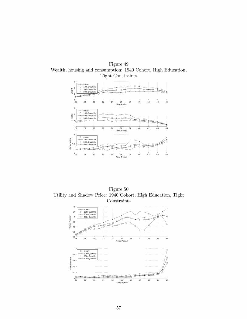
Figure 49Wealth, housing and consumption: 1940 Cohort, High Education,
Tight Constraints
26 28 30 32 34 36 38 40 42 44 460
1
2
3
T ime Period
Wea
lth
mean10th Quantile50th Quantile90th Quantile
26 28 30 32 34 36 38 40 42 44 460
1
2
3
T ime Period
Hou
sing
mean10th Quantile50th Quantile90th Quantile
26 28 30 32 34 36 38 40 42 44 460
0.5
1
T ime Period
Con
sum
ptio
n mean10th Quantile50th Quantile90th Quantile
Figure 50Utility and Shadow Price: 1940 Cohort, High Education, Tight
Constraints
26 28 30 32 34 36 38 40 42 44 4680
60
40
20
0
20
40
T ime Period
Val
ue F
unct
ion
mean10th Quantile50th Quantile90th Quantile
26 28 30 32 34 36 38 40 42 44 460
0.2
0.4
0.6
0.8
1
T ime Period
Sha
dow
Pric
e
mean10th Quantile50th Quantile90th Quantile
57