Applied Mathematics, 2014, 5, 2612-2618 Published Online September 2014 in SciRes. http://www.scirp.org/journal/am http://dx.doi.org/10.4236/am.2014.516249

How to cite this paper: Moustapha, M.V.O. (2014) Heat, Resolvent and Wave Kernels with Multiple Inverse Square Poten-tial on the Euclidian Space n . Applied Mathematics, 5, 2612-2618. http://dx.doi.org/10.4236/am.2014.516249

Heat, Resolvent and Wave Kernels with Multiple Inverse Square Potential on the Euclidian Space n Mohamed Vall Ould Moustapha Unité de Recherche: Analyse, EDP et Modélisation (AEDPM), Département de Mathématiques et Informatique, Faculté des Sciences et Techniques, Université des Sciences, de Technologie et de la Médecine (USTM), Nouakchott, Mauritanie Email: khames@ustm.mr Received 26 June 2014; revised 30 July 2014; accepted 8 August 2014

Copyright © 2014 by author and Scientific Research Publishing Inc. This work is licensed under the Creative Commons Attribution International License (CC BY). http://creativecommons.org/licenses/by/4.0/

Abstract In this paper, the heat, resolvent and wave kernels associated to the Schrödinger operator with multi-inverse square potential on the Euclidian space n are given in explicit forms.

Keywords Heat Kernel, Wave Kernel, Resolvent Kernel, Multiple-Inverse Square Potential, Bessel Function, Lauricella Hypergeometric Function

1. Introduction This article is devoted to the explicit formulas for the Schwartz integral kernels of the heat, resolvent and wave

operators et ν∆ , ( ) 12ν λ

−∆ + and cos t ν−∆ attached to the Schrödinger operator with Multiple-inverse

square potential on the Euclidian space n :

22

2 21 1

1 4n nj

j jj jx xν

ν

= =

−∂∆ = +

∂∑ ∑ (1.1)

where ( )1 2, , , nnν ν ν ν= ∈ .

Note that the Schrödinger operator with bi-inverse square potential in the Euclidian plane is considered in Boyer [1] and Ould Moustapha [2].

M. V. O. Moustapha

2613

For future use we recall the following formulas for the modified Bessel function of the first kind Iν and the Hankel function of the first kind ( )1Hν .

( ) ( )( )

( )1 1 220

2 ee 1 d

π 1 2

zztz

I z t t tν

νν ν

−−= − Γ + ∫ (1.2)

(see Temme [3], p. 237).

( ) ( )( )

20 1, 2,

1x

I x xν

ν νν

→ ≠ − −Γ +

(1.3)

(see Temme [3], p. 234).

( ) ( ) 1 2e 2πxI x x xν− → ∞ (1.4)

(see Temme [3], p. 240).

( ) ( )( )

( ) ( ) 1 21 21

2 2 e 1 dπ 1 2

iztH z z t ti

ννν ν

− −∞−= −Γ − ∫ (1.5)

(see Erdély et al. [4], p. 83).

( ) ( ) ( )2

2 21 2 π 2 2 10

e e dπ

zi ttiiH z t tα

νν νν α α

+ ∞− − − −

= ∫ (1.6)

0mz > and 2 0m zα > (see Magnus et al. [5], p. 84). Recall also that the n variables Lauricella

hypergeometric function ( ) ( ), , ,nAF zα β γ is given by (see Appell et al. [6], p. 114)

( ) ( )( ) ( )( )0

, , ,!

m mn mA

m m

F z zm

α βα β γ

γ= ∑ (1.7)

where ( )1 2, , , nnm m m m= ∈ , 1 2 nm m m m= + + +

, α ∈ ; ( )1 2, , , nβ β β β= , ( )1 2, , , nγ γ γ γ=

and ( )1 2, , , nz z z z=

are in nR . In the sekel we use the integral representation (see Appell et al. [6], p. 115)

( ) ( ) ( ) 11 1 1 1

0 0 011

, , , 1 1 dj j jj n j n

nA j j j j j

jjF z c u u u z u

αγ β βα β γ

−= =− − −

==

= − −

∑∏∫ ∫ ∫ (1.8)

where

( )( ) ( )

1

1

.n

jjn

j j jj

cγ

β γ β=

=

Γ=

Γ Γ −

∏∏

(1.9)

For 2n = we have ( ) ( ) ( )2

2 1 2 1 2 1 2, , , , , , , , ,AF z F z zα β γ α β β γ γ= (1.10)

where 2F is the Apple hyprgeometric function of two variables. Recall also the following formulas for the heat kernel associated to the Schrödinger operator with inverse

square potential 2 2

2 2

1 4Lx xν

ν∂ −= +∂

.

(see Calin et al. [7], p. 68).

( ) ( )2 21 2

4e e2 2

x xtL t

xx xxIt t

νν

′− +′ ′ =

(1.11)

where Iν is the modified Bessel function of the first kind.

M. V. O. Moustapha

2614

Proposition 1.1. The Schwartz integral kernel of the heat operator with multiple-inverse square potential et ν∆ can be written for ( )1 2, , , np x x x=

, ( )1 2, , , nnp x x x +′ ′ ′ ′= ∈ and t +∈ as

( )( ) ( ) ( )

2 21 2

4

1, , e 2

2j j

j

n x x tj jj j

j

x xH t p p I x x t

tν ν

′− +

=

′′ ′=∏ (1.12)

where j

Iν is the modified Bessel function of the first kind and of order jν . Proof. The Formula (1.12) is a direct consequence of the Formula (1.11) and the properties of the operator

(1.1).

2. Resolvent Kernel with Multiple-Inverse Square Potential on the Euclidian Space n

Theorem 2.1. The Schwartz integral kernel for the resolvent operator ( ) 12ν λ

−∆ + is given by the formula.

( ) ( )

( ) ( )

1

1 2 1 1 11 1 0 0 0 2

1

1 2211

1 1

, ,4

4 1 d

j

j

n

nj jj n

j j jj

nn

j j j j j jnj j

G p p c x xp p x x u

H p p x x u u u u

ν

ν

ν

ν

ν

λλ

λ

+ −

+

=

=

−

+ −= =

′ ′=

′ ′ − +

′ ′× − + −

∏ ∫ ∫ ∫∑

∑ ∏

(2.1)

where ( )1Hν is the Hankel function of the first kind and ( )

( ) ( )1 π 21

1 2 2 21

2 eπ 1 2

i n

nn njj

ci

νν

ν ν

− +−

+ − −=

=Γ +∏

.

Proof. We use the well known formula connecting the resolvent and the heat kernels:

( ) ( )2 20

, , e , ; d ; 0.tG p p H t p p t eλν νλ λ

∞′ ′= <∫ (2.2)

We combine the Formulas (2.2), (1.12) and (1.2) then use the Formulas (1.3) and (1.4) to appley the Fubini theorem and in view of the Formula (1.6) we get the Formula (2.1) and the proof of the Theorem 2.1 is finished.

Theorem 2.2. The Schwartz integral kernel of the resolvent operator ( ) 12ν λ

−∆ + can be written as

( ) ( ) ( ) ( ) ( )1 2 222

1, , e , , 2 , dj

nni s

j j Ap pj

G p p c x x s p p F z sαν λ

ν λ α β β−+ ∞

′−=

′ ′ ′= − −∏ ∫ (2.3)

with 1 2 ,nα ν= − + 1 2j jβ ν= + , 22

41, ,j j

j

x xz j n

s p p

′= =

′− − and

( )

( ) ( )( )( )

1 π 22 1

2 11 21

1 22 e2 1π 3 2

i nn n j

nnj

cn i

νν

ν

ν

νν

− ++ −

+ −−=

Γ + = Γ +Γ − −

∏ (2.4)

where ( ) ( ), , 2 ,nAF zα β β is the n-variables Lauricella hypergeometric function given in (1.7).

Proof. We use the Formulas (2.1) and (1.5) as well as the Fubini theorem to arrive at the announced Formula (2.3).

3. Wave Kernel with Multiple-Inverse Square Potential on the Euclidian Space It is known that the energy and information can only be transmitted with finite speed, smaller or equal to the speed of light. The mathematical framework, which allows an analysis and proof of this phenomenon, is the theory the wave equation. The result, which may be obtained, runs under the name finite propagation speed (see Cheeger et al. [8]). The following theorem illustrates the principle of the finite propagation speed in the case of the Schrödinger operator with multiple-inverse square potential.

M. V. O. Moustapha

2615

Theorem 3.1. (Finite propagation speed) Let ( ), ,W t p pν ′ be the Schwartz integral kernel of the wave oper-

ator sin t ν

ν

−∆

−∆, then we have

( ), , 0 whenever .W t p p p p tν ′ ′= − > (3.1)

Proof. The proof of this result use an argument of analytic continuation from the identity

sin 1 e e .2

it itti

ν νν

ν ν ν

−∆ − −∆ −∆ = − −∆ −∆ −∆

(3.2)

We recall the formula [9], p. 50

2 21 2 40

e 1 e e d .π

tut uu u

t

λλ

−∞ − − −= ∫ (3.3)

By setting t ν= −∆ and sλ = in (3.3) we can write

2 4 1 20

1e e e dπ

s us uu uν ν∞− −∆ ∆− −= ∫ (3.4)

and let ( ), ,P s p pν ′ be the integral kernel of e s ν− −∆ then we can write

( ) ( )2 4 1 20

1, , e , , dπ

s zP s p p z H z p p zν ν∞ − −′ ′= ∫ (3.5)

where ( ), ,H z p pν ′ is the heat kernel with the multiple-inverse square potential given by (1.12). Consider the integral

( ) ( ) ( )2 4 1 20

1, , e , , dπ

zJ P p p z H z p p zτν ντ τ

∞ − −′ ′= = ∫ (3.6)

using (1.12) we have

( )( ) ( ) ( )( )

2 22

1 241 4 1 2

01

e e 2 d .π2 j

nnp p sj jj s n

j jnj

x xJ s I x x s sτ

ντ′− +∞= − − −

=

′′=

∏∏∫ (3.7)

From (3.2) we have

( ) ( ) ( )( ) ( ) ( )( )1 1, , , , , , .2 2

W t x x P p p it P p p it J it J iti iν ν ν′ ′ ′= − − = − − (3.8)

Now set

( ) ( ) ( )1 2J J Jτ τ τ= + (3.9)

where

( )( ) ( ) ( )( )

2 22

1 2411 4 1 2

1 01

e e 2 dπ2 j

nnp p sj jj s n

j jnj

x xJ s I x x s sτ

ντ′− += − − −

=

′′=

∏∏∫ (3.10)

( )( ) ( ) ( )( )

2 22

1 241 4 1 2

2 11

e e 2 d .π2 j

nnp p sj jj s n

j jnj

x xJ s I x x s sτ

ντ′− +∞= − − −

=

′′=

∏∏∫ (3.11)

Using the Formula (1.3) we see that the last integral ( )2J τ converge absolutely and is analytic in τ for

1 2 0n ν− + > .

M. V. O. Moustapha

2616

For the first integral ( )1J τ we obtain

( )( ) ( ) ( )( )

2 22

1 241 4 3 2

1 11

e e 2 dπ2 j

nnp p yj jj y n

j jnj

x xJ y I x x y yτ

ντ′− +∞= − − +

=

′′=

∏∏∫ (3.12)

and from the Formula (1.4) we see that

( )( ) ( )( )2 2

1 24 41 3 2

1 1e d

π2

ny p pj jj n

n

x xJ y y

τ ντ′− − +∞= − + +

′=∏

∫ (3.13)

is analytic in τ and converge if 22 0e p pτ ′+ − > , hence the integral ( )J it± is absolutely convergent

if ( ) 22 0it p p′± + − > (i.e.) p p t′− > and in view of (3.8) we have ( ), , 0W t p pν ′ = for p p t′− > and the proof of the Theorem 3.1 is finished.

Theorem 3.2. The Schwartz integral kernel for the wave operator cos t ν−∆ with multiple-inverse square potential on the Euclidian space can be written on the two following forms

( )( ) ( )

1 20 2 21 2 1 2

2 221

, , exp d22 2π j

nnj jj j j n

nj

x x x xuw t p p p p t I u u ut ti tν ν

+= −

−∞=

′ ′ ′ ′= − + −

∏∏∫ (3.14)

and

( )( ) ( )

1 2

2 21 2 1 22 22 0

1, , 2 exp d

22π j

nnj jj j j n

nj

x x x xuw t p p p p t I u u ut ttν ν

∞= −

=

′ ′− ′ ′= − + −

∏∏∫ (3.15)

where j

Iν is the first kind modified Bessel functions of order ν . Proof. We start by recalling the formula (see Magnus et al. [5], p. 73).

( )1 2cos π 2z z J z−= (3.16)

where ( ).Jν is the Bessel function of first kind and of order ν defined by (see Magnus et al. [5], p. 83).

( ) ( )( )20 2 1e d2 π

t z tzJ z t ti

να ν

ν α+ − − −

−∞= ∫ (3.17)

provided that 0eα > and argz ≤ π . Here we should note that the integral in (3.17) can be extended over a contour starting at ∞ , going clockwise around 0, and returning back to ∞ without cutting the real negative semi-axis.

For 1 2ν = − the Equation (3.17) can be combined with Equation (3.16) to derive the following formula.

( )( )20 2 1 21cos e d .2 2π

u z uz u u

iα

α+ − −

−∞= ∫ (3.18)

Putting 1α = and replacing the variable z by the symbol t ν−∆ in (3.18) we obtain

( )( )22 20 1 21cos e d .2 2π

u t ut u u

iν

ν

+ ∆+ −

−∞−∆ = ∫ (3.19)

Finally making use of (1.12) in (3.19), we get the Formula (3.14). To see the Formula (3.15) set

( )0 2 2 2 1 22 2

1exp d

2 j

nj j n

j

x xuJ p p t I u u ut tν

+ −

−∞=

′ ′= − + − ∏∫ (3.20)

and

( )2 2 2 1 22 20

1exp d

2 j

nj j n

j

x xuI p p t I u u ut tν

∞ −

=

′ ′= − + − ∏∫ (3.21)

M. V. O. Moustapha

2617

we have

1 2 3J J J J= + + (3.22)

( )1

2 2 2 1 21 2 2

1exp d

2 j

nj j n

j

x xuJ p p t I u u ut tνγ

−

=

′ ′= − + − ∏∫ (3.23)

( )2

2 2 2 1 22 2 2

1exp d

2 j

nj j n

j

x xuJ p p t I u u ut tνγ

−

=

′ ′= − + − ∏∫ (3.24)

and

( )3

2 2 2 1 23 2 2

1exp d

2 j

nj j n

j

x xuJ p p t I u u ut tνγ

−

=

′ ′= − + − ∏∫ (3.25)

where the paths 1γ , 2γ and 3γ are given by

( )π1 : e ; above the cutiz r rγ = ≤ < ∞

( )π2 : e ; below the cutiz r rγ −= ∞ > ≥

( )3 : e ; π π rund the small circleiz θγ θ= − < <

as 0→ , we have ( )1 21 e n iJ I+ π→ , ( )1 2

2 e n iJ I− + π→ and 3 0J → . Adding the integrals establishes the required results ( )2 sin 1 2J i n I= + π .

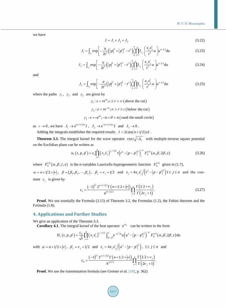
Theorem 3.3. The integral kernel for the wave operator cos t ν−∆ with multiple-inverse square potential on the Euclidian plane can be written as

( ) ( ) ( ) ( ) ( )1 2 223

1, , , , 2 ,j

nn

j j Aj

w t p p c x x t t p p F zαν

ν α β β−+

+=

′ ′ ′= − −∏ (3.26)

where ( ) ( ), , ,nAF zα β γ is the n-variables Lauricella hypergeometric function ( )n

AF given in (1.7),

1 2nα ν= + + , ( )1 2, , , nβ β β β= , 1 2j jβ ν= + and ( )224 1j j jz x x t p p j n′ ′= − − ≤ ≤ and the con-

stant jc is given by

( ) ( )( )

( )( )

1 2

3 1 21

1 21 2 1 2.

2 1π

n n j

nj j

nc

ν ν νν

ν

+ +

+=

Γ +− Γ + +=

Γ +∏ (3.27)

Proof. We use essetially the Formula (3.15) of Theorem 3.2, the Formulas (1.2), the Fubini theorem and the Formula (1.8).

4. Applications and Further Studies We give an application of the Theorem 3.3.

Corollary 4.1. The integral kernel of the heat operator et ν∆ can be written in the form

( ) ( ) ( ) ( ) ( )21 2 24 24

1, , e , , 2 , dj

nnu t

j j Ap pj

cH t p p x x u u p p F z ut

αν

ν α β β−+ ∞ −

′−=

′ ′ ′= − −∏ ∫

with 1 2nα ν= + + , 1 2j jβ ν= + and ( )224j j jz x x u p p′ ′= − − , 1 j n≤ ≤ and

( ) ( ) ( )( )

1 2

4 2 11

1 21 2 1 2.

π 2 1

n n jn

j j

nc

ν ν νν

ν

+ +

+=

Γ +− Γ + +=

Γ +∏

Proof. We use the transmutation formula (see Greiner et al. [10], p. 362)

M. V. O. Moustapha

2618

2 40

1e e cos d .π

t u t u ut

νν

∞∆ −= −∆∫

We suggest here a certain number of open related problems connected to this paper. For example the semi- linear wave and heat equations associated to the multiple-inverse square potential and its global solution and a possible blow up of the solution in finite times.

We can also to look for the dispersive and Strichartz estimates for the Schrödinger and the wave equations with multiple-inverse square potential, for the case of inverse square potential (Burg et al. [11] and Planchon et al. [12]).

References

[1] Boyer, C.P. (1976) Lie Theory and Separation of Variables for the Equation 2 21 2

0tiU Ux xα β

+ + =

. SIAM Journal on

Mathematical Analysis, 7, 230-263. http://dx.doi.org/10.1137/0507019 [2] Ould Moustapha, M.V. (2014) The Heat, Resolvent and Wave Kernels with Bi-Inverse Square Potential on the Eucli-

dean Plane. International Journal of Applied Mathematics, 27, 127-136. [3] Temme, N.M. (1996) Special Functions: An Introduction to the Classical Functions of Mathematical Physics. John

Wiley and Sons, Inc., New-York. [4] Erdélyi, A., Magnus, W., Oberhettinger, F. and Tricomi, F.G. (1954) Transcendental Functions, Tome II. New York. [5] Magnus, W., Oberhettinger, F. and Soni, R.P. (1966) Formulas and Theorems for the Special Functions of Mathemati-

cal Physics. Springer-Verlag, New York. http://dx.doi.org/10.1007/978-3-662-11761-3 [6] Appell, P. and Kampe de Feriet, M.J. (1926) Fonctions Hypergeometriques et Hyperspheriques. Polynôme d’Hermite.

Gauthier-Villars, Paris. [7] Calin, O., Chang, D., Furutani, K. and Iwasaki, C. (2011) Heat Kernels for Elliptic and Sub-Elliptic Operators Methods

and Techniques. Springer, New York. http://dx.doi.org/10.1007/978-0-8176-4995-1 [8] Cheeger, J. and Taylor, M. (1982) On the Diffraction of Waves by Canonical Singularites I. Communications on Pure

and Applied Mathematics, 35, 275-331. http://dx.doi.org/10.1002/cpa.3160350302 [9] Strichartz, R. (2003) A Guide to Distribution Theory and Fourier Transform, Studies in Advanced Mathematics. CRC

Press, Boca Racon. [10] Greiner, P.C., Holocman, D. and Kannai, Y. (2002) Wave Kernels Related to the Second Order Operator. Duke Ma-

thematical Journal, 114, 329-387. http://dx.doi.org/10.1215/S0012-7094-02-11426-4 [11] Burg, N., Planchon, F., Stalker, J. and Tahvildar-Zadeh, A.S. (2002) Strichartz Estimate for the Wave Equation with

the Inverse Square Potential. arXiv:math.AP/0207152v3. [12] Planchon, F., Stalker, J. and Tahvildar-Zadeh, A.S. (2003) Dispersive Estimate for the Wave Equation with the Inverse

Square Potential. Discrete and Continuous Dynamical Systems, 9, 1337-1400.