Health and Income Inequality: An Analysis of Publicversus Private Health Expenditure

Ayona Bhattacharjee ∗ Jong Kook Shin † Chetan Subramanian‡

April 16, 2015

Abstract

This paper examines the link between income inequality and health expenditure

under public and private health regimes. We investigate this issue in a two period

overlapping generations model in which mortality is endogenous and human capital

is the engine of growth.

We find that under the public regime, while rich countries will exhibit high

income growth and low income inequality, poor countries will converge to a vicious

cycle of poor health and low income. Under the private health regime, initial differ-

ences in economic and health status get exacerbated over time. The income growth

rate depends on the initial distribution of income. Finally, we use panel cointe-

gration techniques to assess the impact of public health expenditure on income

inequality.

JEL classification: I14, I15, O11

Keywords: Public and Private Health, Longevity, Income inequality, Growth

∗Department of Economics and Social Sciences, IIM, Bangalore, Bannerghatta Road, Bangalore560076, India, ayona.bhattacharjee10@iimb.ernet.in†Newcastle University Business School, 5 Barrack Road, Newcastle upon Tyne, NE1 4SE, U.K,

jong.shin@newcastle.ac.uk‡Department of Economics and Social Sciences, IIM, Bangalore, Bannerghatta Road, Bangalore

560076, India, chean.s@iimb.ernet.in

1

1 Introduction

This paper contributes to the growing debate on whether the delivery of health care

should be public or private by examining the interplay between health investment and

income inequality under both public and private health care regimes. Our objective is to

examine the role that investment in health plays under the two regimes in explaining the

intergenerational transmission of inequality and its persistence. We examine this issue

in a two period overlapping generations growth model in which mortality is endogenous

and human capital is the engine of growth.

Our work in this paper is motivated by two strands of empirical research. First is

the substantial evidence showing a positive relation between inequality and intergen-

erational correlation of economic status in both developed and developing economies

(Corak 2013). Countries with greater inequality of incomes also tend to be countries

in which there is greater persistence of income across generations. This relationship

between income inequality and income persistence, termed as the “The Great Gatsby

Curve”by Alan Krueger is depicted in Figure 1. The figure ranks countries along two

dimensions. The horizontal axis shows income inequality in a country as measured

by the Gini coeffi cient while the vertical axis has a measure of the persistence of in-

come. Countries like Brazil, China and Chile that have high income inequality tend to

be characterized by high intergenerational correlation in income. On the other hand

countries like Denmark, Norway and Finland which are characterized by low income

inequality tend to have low intergenerational income persistence.

Secondly, there is considerable evidence that points to the fact that poor health

in childhood lowers future income through its effects on schooling and labour force

participation. What is less understood is the effect of the type of health care system

(public vs. private) on health and persistence of income inequality. This is the gap in

the literature that we attempt to address in this paper.

Our paper extends Glomm and Ravikumar (1992) model of endogenous growth, to

include investment in health. Mortality is endogenous in our setup where the length

of life of the adult depends upon the investment in health. Each parent has a bequest

motive and invests in the health of the offspring. Each agent’s stock of human capital

1

depends on the parent’s stock of human capital, time spent in school, and parental

investment in health. As in Glomm and Ravikumar (1992), under the public health

regime, a government levies taxes on the income of the old and uses tax revenues

to provide “free” public health. Public health investment is therefore an increasing

function of the tax revenues. Under the private health regime, every parent decides on

the health investment to be made on the offspring.

The linkage across generations in our model stems from two distinct channels.

Firstly, as mentioned earlier, the stock of human capital of the parent directly af-

fects the human capital stock of the young. Secondly, the stock of human capital of

the parent indirectly affects the human capital accumulation choices of the young by

impacting their old age longevity. The lower the stock of human capital of the older

generation, the lower is the amount they invest in the health of their progeny. The

consequent reduction in length of life increases the rate at which children discount the

future, thereby impacting their investment in human capital.

We begin by comparing the equilibrium paths of per capita income for the two

health regimes when the distribution of income is degenerate. Our results show the

existence of multiple steady states under both regimes depending on the initial levels of

income. High mortality reduces returns on education which results in lower income and

“poverty traps”under both regimes. Interestingly, we find that the threshold “growth

takeoff”income levels are lower and per capita incomes are higher in the private when

compared to the public regime. Intuitively, in the private health regime, each individual

accounts for the fact that an additional unit of time spent toward learning increases

her future earnings and thereby her ability to invest in health of her offspring. In

the public health regime, the latter benefit is not taken into account. This results in

underinvestment in human capital under the public regime.

Next, we seek to understand the impact of health investment on income inequality

under the two health regimes. We demonstrate that in an economy where the income

distribution is skewed and per-capita income is above a threshold, income inequality

decreases over time under the public regime whereas it increases under the private

regime. Intuitively, in such an economy with a high per capita income, expenditure

2

on health under the public regime is high. The higher old age longevity incentivises

increased investment in human capital by the young. In particular, due to diminishing

returns to human capital, low income individuals enjoy higher earnings growth than

high income individuals in transition causing income inequality to shrink under this

regime. By contrast, under the private regime high income individuals invest more in

health and grow faster whereas low income individuals get stuck in the vicious cycle

of poor health and low income. Hence any differences in the initial level of income are

exacerbated over time under the private regime.

It also follows that when the initial per capita income is low, health expenditure

under the public regime tends to be low, leading to a vicious cycle of poor health

and low income for all individuals in the economy. Since all individuals in the econ-

omy converge to low income equilibrium, income inequality falls over time under this

regime. Under the private regime once again, income inequality would rise, with high

income individuals converging to high income growth rates and low income individuals

experiencing falling incomes over time.

This paper is linked to a growing volume of literature that has sought to examine

the link between income inequality and income growth. While traditional channels have

mainly focused on credit market constraints and non-convexities in technology (Galor

and Zeira 1993, Piketty 1997 and others), the role of health in explaining income in-

equality has been less explored. Chakraborty (2004), in a seminal paper explores the

link between public health expenditure and economic growth. Castelló-Climent and

Doménech (2008) and Chakraborty and Das (2005) extend the work of Chakraborty

(2004) to examine the link between income inequality and health in an endogenous

growth framework. Chakraborty and Das (2005) introduce endogenous mortality and

accidental bequests in an otherwise standard overlapping generations model with pro-

duction; in particular, the probability with which a young agent survives into old

age depends on the private health investment made by the young. Owing to lower

longevity, children from poorer households are more likely to receive low bequests and

the resultant wealth effect sets off a cycle of poor health and income. Castelló-Climent

and Doménech (2008) quantitatively and empirically analyze the relationship between

3

inequality in the distribution of education, life expectancy and human capital accumu-

lation. Our paper complements both these papers and focuses instead on the dynamics

of income inequality under private and public health regimes. The key linkage between

generations in our model occurs through parental investment in the progeny’s health

and we abstract away from issues related to accidental bequests.

Moreover, this paper also contributes to the emerging empirical literature that

analyses the influence of health expenditure on income inequality. A number of papers

have examined the link between income inequality and health outcomes (See Deaton,

2003 for a review). Our work complements this literature by examining the link between

public health spending and income inequality.1 We examine this issue using data from

a sample of OECD countries. There are two key empirical issues in the literature

which we attempt to address in this paper. Firstly, several studies have pointed to

the possible non-stationarity in health care spending and income inequality (Baltagi

and Moscone 2010, Herzer and Nunnenkamp 2014 and others). Secondly, when income

and health interactions are important, health can not only be a consequence but can

also be a cause of income inequality. This issue of endogeneity is something that the

literature has pointed out but not addressed adequately. Our work addresses both

these issues by applying panel cointegration techniques. Results show a statistically

significant negative long-run effect of public health spending on Gini coeffi cient. These

appear consistent with our theoretical findings.

The rest of the paper is structured as follows: Section 2 discusses the theoretical

model, with the private and public health regimes discussed in Sections 2.1 and 2.2

respectively. Section 2.3 looks at outcomes for homogeneous individuals and Section 2.4

illustrates the same for heterogeneous individuals. Section 3 is the empirical evidence

for a proposition of the model. Section 3.1 discusses the empirical strategy of using

panel cointegration. Section 3.2 discusses the preliminary results in support of our

proposition. Section 4 contains the concluding remarks.

1Such a relation has been studied in the context of education. Glomm and Ravikumar (1992)theoretically show declining income inequality in a public education regime.

4

2 Model

Our model and its structure follow Glomm and Ravikumar (1992). We extend their

two-period overlapping generations framework to include endogenous mortality. We

abstract away from issues related to fertility or population growth and assume that at

the end of one’s youth an individual gives birth to a single offspring. Individuals born

at time period t have identical preferences over leisure when young, consumption when

old, and the opportunity to invest in health of their offspring.

All young individuals survive to the second period but are alive only for a fraction

φ(.) of the second period.2 We term φ(.) as the longevity function, which depends

on the health investment incurred by the parental generation. As in Bhattacharya

and Qiao (2007) we interpret these as preventive medicines that extend the length of

life. These investments may be privately or publicly funded. We assume a constant

elasticity form for φ. It is strictly increasing and concave in health spending.

φ(.) with φ(0) = 0; φ′ > 0; φ′′ ≤ 0; limh→∞φ(h) = φ ≤ 1

We follow the literature in assuming the longevity function to be,

φ(h) = Ahε for h < h (1)

φ(h) = φ for h > h

where A > 0, indicates the state of medical technology. h is the health investment,

with returns given by ε lying between (0, 1). The parameter φ denotes the maximum

longevity (under current medical technology) and (h, e) is the corresponding critical

level of health investment and earnings.

Under the public health regime, the health investment on the young in time period t

is financed by levying a tax on the income of the old. Under this regime, all individuals

face the same health care investment. By contrast, in the case of private health regime,

2As in Bhattacharya and Qiao (2007), ours is a model of longevity in old age as opposed to child orinfant mortality. This allows us to abstract away from issues relating to unintended bequests, which isthe focus of Chakraborty and Das (2005).

5

every adult allocates her income between own consumption and health investment on

her offspring. Young individuals at time t accumulate human capital, et+1 according

to,

et+1 = ξ (1− nt)eδthνt (2)

where et is the stock of human capital of the corresponding parent. ξ denotes the

productivity parameter associated with human capital accumulation. The income of

the individual during the second period of life is equal to the stock of human capital,

et+1. When young, individuals allocate nt units of their unit time endowment towards

leisure and the remaining towards accumulating human capital. Parental knowledge

and health are also critical inputs in our human capital accumulation equation. The

importance of parental knowledge as an input in the process of human capital accu-

mulation is a feature that has been well documented. The seminal work by Becker

and Tomes (1979) attribute intergenerational income persistence not only to genetic

factors but also to parental human capital. Recent work by Black and Devereux (2011)

has highlighted the link between parental human capital and income persistence. The

effect of health status on human capital accumulation is also well established. Numer-

ous studies have shown that poor health adversely affects cognitive skills, productivity

and educational outcomes. Currie and Hyson (1999) use British cohort data and find a

positive relation between birth weight and educational outcomes. More recently, Figlio

et.al (2013) using US data provide evidence on the long-term effects of birth weight

on cognitive development. They find that increases in birth weight can have a positive

effect on cognitive skills, and hence on adult earnings.

2.1 Private Health Regime

Formally, the preferences of an individual born at time t is represented by

U = ln(nt) + φ(ht)[ln(ct+1) + αln(ht+1)] (3)

where nt is leisure at time t, ct+1 is consumption at time t+ 1, and ht+1 is the health

investment at time t + 1. The parameter α captures parental altruism. The budget

6

constraint is then given by

et+1 = ct+1 + ht+1 (4)

The optimisation follows a two-step maximisation procedure. In the first step, an

individual maximizes her second period utility function subject to the budget constraint

to obtain

ct+1 =1

1 + αet+1; ht+1 =

α

1 + αet+1 (5)

Both second period consumption and health investment by the adult are a rising func-

tion of human capital. From equation (5), it follows that health investment varies

positively with the degree of altruism, α. In the second step we substitute the optimal

level of second period consumption and health spending back into the lifetime utility

function and solve for optimal leisure to obtain

nt =1

1 + (1 + α)φ(ht)(6)

Equation (6) shows that leisure choice varies inversely with parental health expenditure,

dntdht

< 0. Intuitively, with a rise in health expenditure, the longevity of the young rises,

thereby incentivising investment in human capital.

Next we proceed to formulate the human capital accumulation equation under the

private health regime. Unlike most of the literature which assumes some form of non-

convexity of technology to study the issue of development traps, we assume constant

returns to scale, i.e. δ + ν = 1. Substituting equations (5) and (6) into equation (2)

gives,

J(et) = et+1 =

θ1θ2e

ε+1t

1+θ1eεtfor eϕ ≤ et < e

θ1θ2eε

1+θ1eεet for et ≥ e

(7)

where θ1 = A( α1+α)ε(1 + α) and θ2 = ξ( α

1+α)ν are positive constant terms. Notice that

J′(e) > 0 for any e; J

′′(e) > 0 for e < e ; but J

′′(e) = 0 for e ≥ e. The above equation

indicates that the income locus has a convex portion till the critical health spending h

(corresponding to e), is reached, beyond which the locus starts following a linear path.

7

2.2 Public Health Regime

Under the public regime an individual takes health spending as given and chooses nt

and ct+1 to maximize

U = ln(nt) + φ(Ht)[ln(ct+1) + αln(Ht+1)] (8)

subject to,

ct+1 = (1− τ t+1)et+1 (9)

where τ t+1 is the income tax rate imposed on the adults in period t+ 1; Ht+1 is public

health spending in period t+1 and is given by τ t+1Et+1 where Et+1 =∫et+1dFt+1(et+1)

is the per capita earnings as of period t + 1 and F denotes the earnings distribution.Following Glomm and Ravikumar (1992), we solve for the preferred tax rate by max-

imising the second period utility,

[ln((1− τ t+1)et+1) + αln(τ t+1Et+1)]

to obtain

τ t+1 =α

1 + α, (10)

The optimal tax rate is therefore independent of the level of individual income and is

constant over time. It varies positively with α, indicating the more altruistic a society

is the higher the tax individuals are willing to pay. On substituting equation (10) into

equation (9) we find the second period optimal consumption level is,

ct+1 =1

1 + αet+1 (11)

It is easy to see that the time allocated to leisure under the public regime is,

nt =1

1 + φ(Ht)(12)

8

Unlike in the private health regime, individuals here do not factor health investment

on their progeny. They therefore compare only the marginal benefit of leisure with

marginal cost of future consumption. The opportunity cost of leisure consumption

being lower makes the individuals invest lesser time for education in this regime. This

results in lower future stream of income under the public regime. Substituting equations

(10) and (12) into equation (2) gives,

M(et, Et) = et+1 =

θ2θ3E

ε+νt eδt

1+θ3Eεtfor eϕ ≤ Et < e

θ2θ3eε

1+θ3eεEνt e

δt for Et ≥ e

(13)

where θ3 = A(

α1+α

)ε< θ1. To facilitate comparison of this income locus with that

under the private regime, consider the case of homogeneous individuals under which,

Et = et. Notice that in this case, it follows from equation (13), M′(e) > 0 for any e;

M′′(e) > 0 for e < e; but M

′′(e) = 0 for e ≥ e. Therefore, as in the private regime, the

income locus has a convex portion till the critical human capital, e is reached, beyond

which the locus starts following a linear path.

2.3 Homogeneous individuals

The objective of this section is to analyse the paths of earnings under the two health

regimes when individuals are homogeneous. The problem therefore reduces to com-

paring equations (7) and (13) which are the income loci under the private and public

regimes respectively. The key results are summarised in the proposition below,

Proposition 1 Under the assumption of homogeneous individuals in the economy with

the same initial level of income,

(A) Per capita income is lower in the public regime compared to the private regime

(B) The threshold income at which the private regime (er = [θ1 (θ2 − 1)]−1ε > 0) en-

ters into endogenous sustained growth is less than that in the public regime (eu =

[θ3 (θ2 − 1)]−1ε > 0)

(C) Under endogenous sustained growth path (e ≥ e), the income growth rate under the

private regime (gr = θ1θ2eε

1+θ1eε) is higher than under the public regime (gu = θ2θ3eε

1+θ3eε)

9

Proof. See Appendix A.1

Figure 2 plots the income loci under the two regimes. The dotted line represents

the private income locus and the solid line represents the public income locus. If indi-

viduals start off with the same human capital under the two regimes, human capital

accumulation under the private regime will always be greater than that in the pub-

lic regime. The young under the private regime take into account the fact that their

health investment impacts the income of their progeny. This in turn leads to higher

time investment for accumulating human capital compared to the public regime. As

individuals choose to accumulate less human capital under the public regime, the econ-

omy requires higher initial income to attain the sustained endogenous growth path.

Once the income crosses the critical level and attains endogenous growth, the long-run

income growth rate becomes constant. This growth rate is higher under the private

compared to the public regime. Once again this is due to the fact that under the private

regime health investments are fully internalised unlike the public regime.

Interestingly, if we assume away the endogenous longevity function, our model will

not generate income persistence results. In this case φ(.) is assumed to be a constant,

and hence leisure no longer responds to health investments. Without loss of generality,

we assume φ = 1 for this analysis. The income loci under the two regimes get modified

to,

J(et) = et+1 = ξ1 + α

2 + α

(α

1 + α

)νet ≷ et under the private regime (14)

M(et) = et+1 = ξ1

2

(α

1 + α

)νet ≷ et under the public regime.

Equation (14) denotes the income locus in each case. Depending on the magnitude

of the coeffi cients on et, two cases may arise. It follows that in either case, the path

of income is independent of the initial level of human capital, thus no persistence in

earnings over generations.

We next proceed to discuss the steady states and their stability properties under

the two regimes. This can be summarised in the Proposition below,

Proposition 2 The dynamic system described by equations (7) and (13) may possess

10

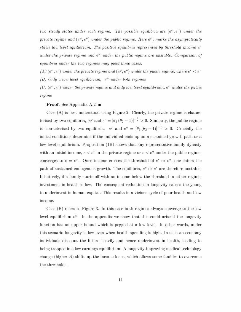
two steady states under each regime. The possible equilibria are (eϕ, er) under the

private regime and (eϕ, eu) under the public regime. Here eϕ, marks the asymptotically

stable low level equilibrium. The positive equilibria represented by threshold income er

under the private regime and eu under the public regime are unstable. Comparison of

equilibria under the two regimes may yield three cases:

(A) (eϕ, er) under the private regime and (eϕ, eu) under the public regime, where er < eu

(B) Only a low level equilibrium, eϕ under both regimes

(C) (eϕ, er) under the private regime and only low level equilibrium, eϕ under the public

regime

Proof. See Appendix A.2

Case (A) is best understood using Figure 2. Clearly, the private regime is charac-

terised by two equilibria, eϕ and er = [θ1 (θ2 − 1)]−1ε > 0. Similarly, the public regime

is characterised by two equilibria, eϕ and eu = [θ3 (θ2 − 1)]−1ε > 0. Crucially the

initial conditions determine if the individual ends up on a sustained growth path or a

low level equilibrium. Proposition (1B) shows that any representative family dynasty

with an initial income, e < er in the private regime or e < eu under the public regime,

converges to e = eϕ. Once income crosses the threshold of er or eu, one enters the

path of sustained endogenous growth. The equilibria, eu or er are therefore unstable.

Intuitively, if a family starts off with an income below the threshold in either regime,

investment in health is low. The consequent reduction in longevity causes the young

to underinvest in human capital. This results in a vicious cycle of poor health and low

income.

Case (B) refers to Figure 3. In this case both regimes always converge to the low

level equilibrium eϕ. In the appendix we show that this could arise if the longevity

function has an upper bound which is pegged at a low level. In other words, under

this scenario longevity is low even when health spending is high. In such an economy

individuals discount the future heavily and hence underinvest in health, leading to

being trapped in a low earnings equilibrium. A longevity-improving medical technology

change (higher A) shifts up the income locus, which allows some families to overcome

the thresholds.

11

Case (C) corresponds to the case of only low level equilibrium under the public

regime and multiple equilibria in the private regime (see Figure 4). This case arises

when the maximum attainable longevity is bounded between the values defined in

Cases (A) and (B). For such intermediate levels of medical infrastructure, the private

regime could potentially enter a path of sustained growth, whereas the public regime

would always converge to the low level equilibrium irrespective of its initial level of

income. Our results indicate that the “state of medical infrastructure”as proxied by

the longevity function in an economy, is a key determinant of the income dynamics. In

countries with intermediate levels of medical infrastructure, the private regime appears

to outperform a public regime. On the other hand if the state of medical infrastructure

is well developed both public and private regimes exhibit similar income dynamics. If

the initial income is greater than a given threshold then economies under both regimes

converge to sustained growth paths. Recall that gr > gu, the private regime has a

higher growth rate than the public regime, given homogeneous population (Proposition

1C). In the next section we relax the assumption of homogeneous individuals to discuss

the impact of health investment on income inequality.

2.4 Heterogeneous individuals

In this section we compare the income inequality dynamics when the initial income

distribution is not degenerate.3 Proposition 3 summarises the results pertaining to the

two regimes.

Proposition 3 (A) Under the private health regime, income inequality rises over time

(B) Under the public health regime, income inequality declines over time

Proof. See Appendix A.3

We restrict our attention to the case where we have multiple equilibria under both

regimes (case A from A.2). Consider the case of a private regime (see Figure 5). If

income is less than the threshold er, one’s income growth rate would be negative,

resulting in income converging to the low level equilibrium. On the other hand if

3 Irrespective of the health regime under study, we ignore the trivial case of all individuals lying onthe same side of an income distribution.

12

the income is above the threshold, the income growth rate would be positive and the

individual would eventually be on a sustained growth path. Thus given any initial

income, income of the individuals above the threshold will keep increasing while those

below the threshold will keep decreasing. This will result in an increase in income

inequality.

Next we examine the equilibrium long-run growth rate under the private regime.

Let λ be the proportion of the population with an initial income below the threshold,

er. The long run growth rate is therefore given by,

gr = (1− λ)θ1θ2e

ε

1 + θ1eε(15)

It follows from equation (15) that the higher the value of λ, the lower is the income

growth rate in the economy in the long-run. The income growth rate under the private

regime is therefore crucially dependent on the initial distribution of income.

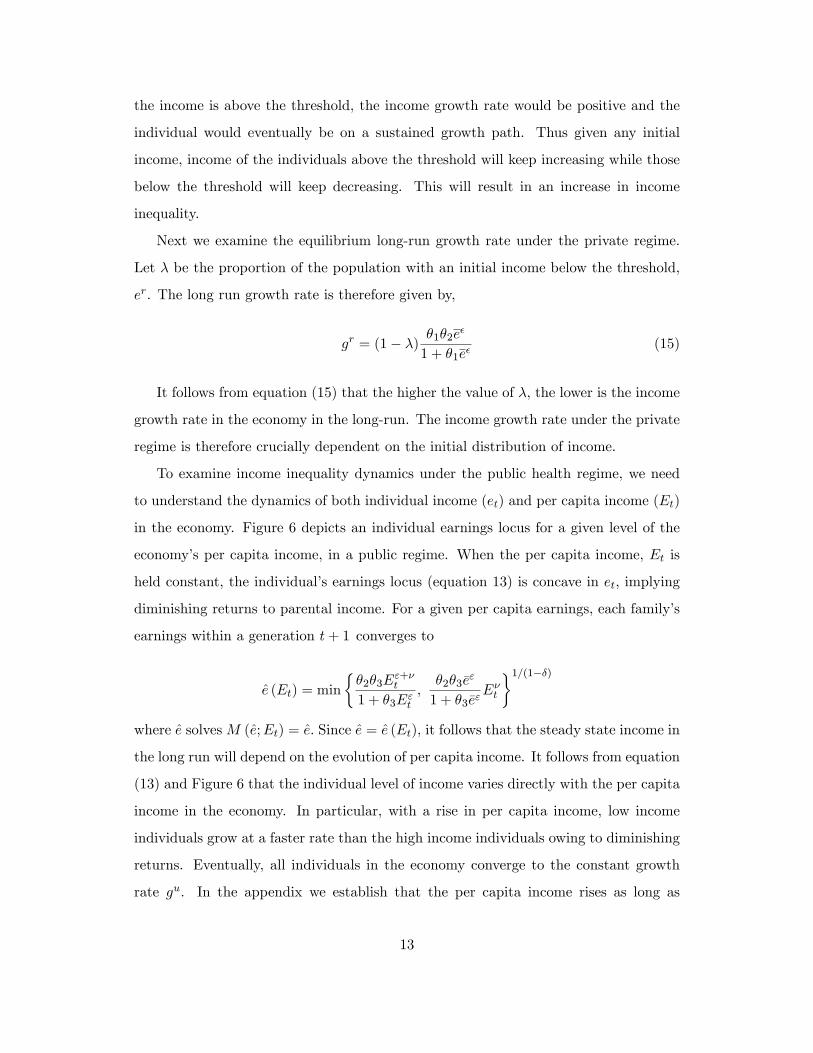
To examine income inequality dynamics under the public health regime, we need

to understand the dynamics of both individual income (et) and per capita income (Et)

in the economy. Figure 6 depicts an individual earnings locus for a given level of the

economy’s per capita income, in a public regime. When the per capita income, Et is

held constant, the individual’s earnings locus (equation 13) is concave in et, implying

diminishing returns to parental income. For a given per capita earnings, each family’s

earnings within a generation t+ 1 converges to

e (Et) = min

{θ2θ3E

ε+νt

1 + θ3Eεt,θ2θ3e

ε

1 + θ3eεEνt

}1/(1−δ)where e solvesM (e;Et) = e. Since e = e (Et), it follows that the steady state income in

the long run will depend on the evolution of per capita income. It follows from equation

(13) and Figure 6 that the individual level of income varies directly with the per capita

income in the economy. In particular, with a rise in per capita income, low income

individuals grow at a faster rate than the high income individuals owing to diminishing

returns. Eventually, all individuals in the economy converge to the constant growth

rate gu. In the appendix we establish that the per capita income rises as long as

13

the initial per capita income is greater than a threshold eu′

= [θ3 (θ2χ0 − 1)]−1ε > eu

where χt =

∫eδtdF (et)/E

δt ≤ 1 measures earnings inequality. The threshold in turn

is negatively related to the initial income inequality, χ0. Under the public regime, the

equilibrium long-run growth rate would depend upon the initial per capita income

and income distribution. If the initial per capita income is greater than eu′, then the

economy converges to a growth rate given by gu = θ2θ3eε

1+θ3eε. It follows from the discussion

above, that unlike the homogeneous case, it is possible that in the heterogeneous case

growth rate under the public regime exceeds that of the private regime. Conversely, if

the initial per capita income is below eu′, the per capita income declines over time and

individual incomes converge to the poverty trap. Importantly, in both these cases, the

income inequality as measured by the dispersion of income is reduced under the public

regime.

Our findings in this section are able to relate the Great Gatsby curve in Figure

1, with the type of the health care system and specifically suggests that high income

countries with predominantly public health regimes, such as Denmark and Norway,

exhibit low income inequality whereas middle income countries such as Brazil and

Chile with largely private health regimes exhibit high income inequality.

We next proceed to test empirically our hypothesis that countries with high per

capita income and predominant public healthcare system will experience decreasing

income inequality. In Section 3, we use data on OECD countries to carry out the

empirical analysis.

3 Empirical Evidence

In this section we try to examine the long-run relation between public health spending

and income inequality. There is large literature which looks at the impact of income

inequality on health outcomes. However our theoretical model shows that as income and

health interact, income inequality and health spending get determined simultaneously.

Even though such endogeneity is commonly acknowledged, not many papers address it

empirically. So we create an empirical framework wherein we show that causality can

14

run both ways. An econometric concern in executing this arises since literature has

shown that these variables are likely to be non-stationary.4 We try to correct for both

these limitations by applying panel cointegration and vector error correction models.

Section 3.1 outlines the basic steps and Section 3.2 summarises the results.5

3.1 Methodology & Data sources

One of the challenges of addressing this problem is the lack of data availability. We

therefore select a group of OECD countries for which data is available for an extended

period of time. Specifically we select a sample of OECD countries with at least 20

continuous annual observations on public health spending and income inequality. Pe-

droni (2004) reports that the nuisance parameters associated with serial correlation

properties are eliminated asymptotically as T grows large relative to N . Hence we give

more importance to the time dimension and ensure that T is suffi ciently larger than

N . Our bivariate regression of interest is,

Giniit = ηi + %it+ β(Public health expenditure)it + εit (16)

i = 1, 2, . . . , N denotes the number of OECD countries as the cross-sectional units,

and t = 1, 2, . . . ., T represents the time periods. We use two samples of 8 countries

each. We restrict our sample years to either 1980-2011 or 1988-2011, depending on

data availability in each case.

Gini is a proxy for income inequality. The intercept ηi controls for country-specific

time invariant factors. %i represents the country-specific time trends. β captures the

permanent change in the income inequality measure associated with a unit percentage

increase in public health spending share.

We use cross-country Gini coeffi cients from a recently developed dataset, the Stan-

dardized World Income Inequality Database SWIID (2013) by Solt (2009). The SWIID

dataset was developed using a missing-data algorithm to standardise the Luxembourg

4Several studies point to the possible non-stationarity of health care spending and income inequality.Non-stationary variables may yield spurious regressions.

5We execute all our econometric exercises on EVIEWS8.

15

Income Study (LIS) and the World Income Inequality Database (WIID). The indices

are reported on a scale of 0 to 100 with higher values indicating higher extent of

income inequality. We obtain public health expenditure from the OECD Health Sta-

tistics (2014). We proxy for the public health share by the percentage of public health

expenditure in total health expenditure (henceforth represented as PUBHE).

The public health expenditure and the inequality measures are assumed non-stationary

integrated processes. We verify this assumption from panel unit root tests. Then we

use the Pedroni cointegration test to check for presence of any long-run relation. We

address endogeneity by using fully modified OLS (FMOLS) estimator. The residuals

from FMOLS are then used in the panel vector error correction model (PVECM).

As a final step we use the error correction mechanism (equation 17). When two

variables are cointegrated, at least one of them adjusts next period to correct for the

disequilibrium. We estimate the following PVECM,4Giniit = η1i + λ1iei,t−1 +

∑j β11ij4Ginii,t−j +

∑j β12ij4PUBHEi,t−j+ε1i,t

4PUBHEit = η2i + λ2iei,t−1 +∑

j β21ij 4Ginii,t−j+∑j β22ij4PUBHEi,t−j + ε2i,t

(17)

where 4 represents the first difference. η1i and η2i are the intercept terms; λ1i and λ2i

are the speeds of adjustments; ei,t−1 is the disequilibrium error term from the previous

period estimated via FMOLS. β represents the respective slope coeffi cients, ε1i,t and

ε2i,t are the white noise terms.

3.2 Empirical results

Table 1 provides details on each sample. The samples are classified mainly by data

availability. Canada, Finland, Norway, Spain and Sweden are in both samples, Nether-

lands, Denmark, the Republic of Korea are only in Sample 1 whereas Austria, Italy and

Switzerland are only in Sample 2. Covering the time period between 1980-2011, Sample

1 uses Gini coeffi cient of disposable income. Sample 2 uses the Gini coeffi cient of total

income over 1988-2011 period. Table 2 provides the average values of the variables over

16

the respective time periods. All countries in our samples had more than 50% of total

health spending provided by public sources, except the Republic of Korea.

We begin by checking the stationarity of variables. To this end, we follow Levin

et.al (2002, LLC) and Im et.al (2003, IPS) panel unit root tests. The LLC unit root

test allows for fixed effects and individual deterministic trends. The null hypothesis of

this test is that each individual time series contains a unit root against the alternative

that each time series is stationary. One problem with this methodology is that rejection

of the null would imply that the autocorrelation coeffi cient across all countries is the

same. The IPS test overcomes this problem by averaging ADF tests. This test allows

for heterogeneous coeffi cients. The null hypothesis of the IPS test is that each series has

a unit root against the alternative that some of the individual series have unit roots. In

other words there are at least some cross-sectional units which have a stationary series

but not necessarily all. Since ours is a cross-country balanced data, we use both LLC

and IPS tests and check if the variables are I(1) processes.

Panel unit root tests in each sample with individual intercept and trend are reported

in Table 3. The two variables in each sample are non-stationary at levels but stationary

at first difference. Thus the unit root test statistics indicate that the two variables follow

I(1) processes. A caveat is that we do not assume either income inequality or public

health expenditure to be inter-related across our sample of countries. So we do not

correct for any cross-sectional dependence.

Any two variables are said to be cointegrated when they share a common stochastic

drift. Pedroni (2004) extended the Engle-Granger two step residual based procedure

to test for the null of no cointegration. This test provides “panel” and “group” test

statistics. The panel statistics assume that the first order autoregressive parameters

are same for all countries. Rejection of the null hypothesis implies that the variables

are cointegrated for all the countries. The group statistics allow for heterogeneous

autoregressive parameters. The alternative is in favour of cointegration for at least one

country. Following Pedroni (2004), we use the group and panel ADF tests only, since

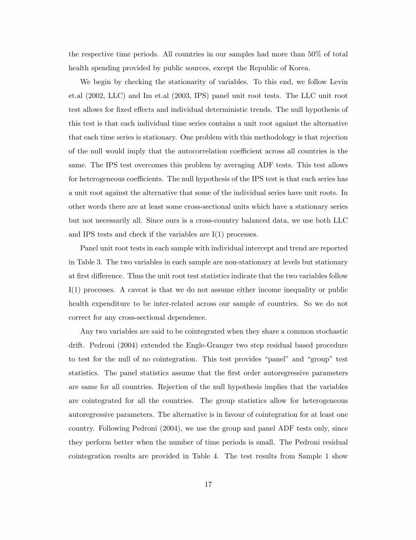
they perform better when the number of time periods is small. The Pedroni residual

cointegration results are provided in Table 4. The test results from Sample 1 show

17

that the null hypothesis of no cointegration is rejected around 10% level of significance.

Although the unweighted ADF cannot reject the null at 10%, its p-value barely exceeds

10% (0.118). Sample 2 shows stronger statistical significance. All tests reject the null

of no cointegration at 5%. The test based on group ADF statistics rejects the null at

1%.

Given the evidence of long-run linear relationship between income inequality and

public health expenditure, we estimate the equilibrium equation using FMOLS. As

mentioned earlier, our model indicates possible endogeneity between public health ex-

penditure and earnings inequality. To address endogeneity problem, literature has

largely employed the use of instrumental variables (IV). As it is diffi cult to find an ap-

propriate IV for a panel setting here, we apply FMOLS (Pedroni, 2001) to correct for

endogeneity and serial correlation. Table 5 reports the FMOLS results. The negative

effect of public health expenditure on inequality is evident in both the samples. The

coeffi cient is statistically significant.

Table 6 reports the results. The first and third columns indicate causality running

from public health spending to the respective inequality measure. The second and

fourth columns indicate causality from income inequality to public health spending.

The statistically significant coeffi cient of the cointegrating vector in the first and third

columns indicate that previous disequilibrium in income inequality is corrected every

period. The short-run effects of public expenditure are however insignificant. This

shows that public health spending and income inequality have a long-run rather than a

short-run relation. When checking for the other direction of causality, from inequality

to public health spending, we observe statistically insignificant coeffi cients. Further

the estimated λ2i is about one order of magnitude smaller than λ1i. It can thus be

concluded that public health spending is weakly exogenous and has a long-run negative

causal effect on income inequality. This effect is consistent with our theoretical result

of declining income inequality under the public health regime. Our finding specifically

implies that measures which equalize health conditions across the population, are likely

to narrow the income distribution.

18

4 Conclusion

In this paper we seek to explain the persistence of health status and income inequality

across generations. Specifically, we contrast the dynamics of the economy under a

public and a private health care regime. We show that under the private regime,

income inequality generally rises; with the affl uent converging to high income growth

and the lower income segment getting stuck in a vicious cycle of poor health and low

income growth. By contrast, income inequality always falls under the public health

regime. It is however worth noting that all individuals under the public regime end up

converging to either a “high”growth or a “low”growth equilibrium depending upon

the initial distribution of income. In other words, reduced income inequality could be

potentially accompanied by a low income growth rate under a public regime.

Interestingly, our analysis would suggest that should the state of medical infrastruc-

ture as proxied by our longevity function be “good” and the income distribution be

such that the initial per capita income is suffi ciently high, the public regime would be

preferred by a majority of the population. We establish that under these circumstances

the public regime would result in an increase in longevity while reducing income in-

equality. The private regime on the other hand would also see increased longevity for a

section of the population but this might come at the cost of higher income inequality.

However, in the case where the state of medical infrastructure is “intermediate”, the

public regime would result in all individuals in the economy converging to a low income,

poor longevity equilibrium. The private health regime on the other hand would deliver

high growth and longevity for the high income individuals.

Empirically, we use data from a group of OECD countries where health care spend-

ing is predominantly public to investigate the relationship between health expenditure

and income inequality. We do find evidence that suggests that higher public health

expenditure leads to a decline in income inequality over time in these countries.

One critical handicap that we face in understanding the relation between health

expenditure and income inequality is the lack of data availability for an extensive

period. This is particularly the case for developing countries. Ideally, we would also like

to investigate how the share of private health expenditure impacts income inequality.

19

This would then help us test the validity of our theoretical predictions more directly.

We leave this for future research.

20

References

[1] Baltagi, B. H. and F. Moscone (2010). Health care expenditure and income in the

OECD reconsidered: Evidence from panel data. Economic Modelling 27 (4), 804-

811.

[2] Becker, G. S. and N. Tomes (1979). An equilibrium theory of the distribution

of income and intergenerational mobility. Journal of Political Economy 87 (6),

1153-1189.

[3] Bhattacharya, J. and X. Qiao (2007). Public and private expenditures on health

in a growth model. Journal of Economic Dynamics and Control 31 (8), 2519-2535.

[4] Black, S. E. and P. J. Devereux (2011). Recent developments in intergenerational

mobility. Handbook of labor economics Volume 4, 1487-1541.

[5] Castelló-Climent, A. and R. Doménech (2008). Human capital inequality, life ex-

pectancy and economic growth. The Economic Journal 118 (528), 653-677.

[6] Chakraborty, S. (2004). Endogenous lifetime and economic growth. Journal of

Economic Theory 116, 119-137.

[7] Chakraborty, S. and M. Das (2005). Mortality, Human Capital and Persistent

Inequality. Journal of Economic Growth 10, 159-192.

[8] Corak, M. (2013). Income inequality, equality of opportunity, and intergenerational

mobility. The Journal of Economic Perspectives, 79-102.

[9] Currie, J. and R. Hyson (1999). Is the impact of health shocks cushioned by

socioeconomic status? The case of low birthweight. National Bureau of Economic

Research.

[10] Deaton, A. (2003). Health, inequality and economic development. Journal of Eco-

nomic Literature 41, 113-158.

21

[11] Figlio, D. N., J. Guryan, K. Karbownik, and J. Roth (2013). The effects of poor

neonatal health on children’s cognitive development. National Bureau of Economic

Research.

[12] Galor, O. and J. Zeira (1993). Income distribution and macroeconomics. The re-

view of economic studies 60 (1), 35-52.

[13] Glomm, G. and B. Ravikumar (1992). Public versus Private investment in Human

Capital: Endogenous growth and Income Inequality. Journal of Political Economy,

818-834.

[14] Herzer, D. and P. Nunnenkamp (2014). Income inequality and health: Evidence

from developed and developing countries.

[15] Im, K. S., M. H. Pesaran, and Y. Shin (2003). Testing for unit roots in heteroge-

neous panels. Journal of econometrics 115 (1), 53-74.

[16] Levin, A., C.F. Lin, and C.S. James Chu (2002). Unit root tests in panel data:

asymptotic and finite-sample properties. Journal of econometrics 108 (1), 1-24.

[17] OECD Health Statistics, 2014.

[18] Pedroni, P. (2000). Fully modified OLS for heterogeneous cointegrated panels in

Nonstationary Panels, Panel Cointegration and Dynamic Panels, Volume 15, Pages

93-130.

[19] Pedroni, P. (2004). Panel cointegration: asymptotic and finite sample properties of

pooled time series tests with an application to the PPP hypothesis. Econometric

theory 20 (03), 597-625.

[20] Piketty, T. (1997). The dynamics of the wealth distribution and the interest rate

with credit rationing. The Review of Economic Studies 64 (2), 173-189.

[21] Solt, F. (2009). Standardizing the world income inequality database. Social Science

Quarterly 90 (2), 231-242.

22

A Appendix

In this section, we provide proofs of the propositions.

A.1 Proof of Proposition 1

For this proposition, we focus on the homogenous agent case in which et = Et for allindividuals.

Proposition (1A)Given that θ1 > θ3, it follows from (7) and (13) that J (e) > M (e) and J ′ (e) >

M ′ (e) for any e.

Proposition (1B)If the economy does not reach the threshold earnings over the convex part (e < e),

it can never enter the sustained growth path. Therefore, the threshold value must lieon the convex part of the earnings locus. To see this, consider the private regime.When J(e) ≥ e, J (e) is on or above the 45 degree line. This implies that the growthrate for e ≥ e is J ′ (e) ≥ 1. This means a sustained constant growth in steady state.Conversely, if J(e) < e, J ′ (e) < 1. Thus the growth rate for e < e is negative.

To obtain the threshold level of earnings, we set et+1 = J(et) = et. Solving for etusing the convex part of J , we get

ert =

[1

θ1 (θ2 − 1)

] 1ε

> 0 (A.1)

for the private regime. Similarly, under the public regime the threshold income isattained when,

eut =

[1

θ3 (θ2 − 1)

] 1ε

> 0 (A.2)

Comparing equations (A.1) and (A.2), we see that, ert < eut because θ1 > θ3. Thusthe threshold earnings to attain sustained endogenous growth is higher under the publicregime.

Proof of Proposition (1C)J (e) > M (e) for any e also implies this. Furthermore, J and M imply that the

earnings growth rates et+1et

along the sustained growth paths are,

gr =θ1θ2e

ε

1 + θ1eε(A.3)

under the private regime and

gu =θ3θ2e

ε

1 + θ3eε(A.4)

23

under public regime. Clearly, gr > gu because θ1 > θ3.

A.2 Proposition 2

Proposition (2A)The case of (eϕ, er) and (eϕ, eu) under the private and the public regimes can happen

ifJ ′(e) > M ′(e) ≥ 1.

Given Proposition 1, the first part is satisfied when, M ′(e) =ξ A( α

1+α)ε+νeε

1+A( α1+α

)εeε ≥ 1,

which implies that

φ ≥ 1

ξ( α1+α)ν − 1

= φ1 (A.5)

i.e. when the highest attainable longevity is greater than the above specified level.

Proposition (2B)The case of only a low level equilibrium under both regimes may arise when

1 > J ′(e) > M ′(e)

This case requires J ′(e) =ξ A( α

1+α)ε+ν(1+α)eε

1+A( α1+α

)ε(1+α)eε < 1 and thus,

φ <1

{ξ( α1+α)ν − 1}(1 + α)

= φ2 < φ1 (A.6)

i.e. when the highest attainable longevity is less than the above specified level.

Proposition (2C)This can arise if,

J ′(e) > 1 and M ′(e) < 1 (A.7)

Combining cases (A) and (B), the case of (eϕ, er) under the private regime and onlyeϕ under the public regime may arise. This can happen if the maximum attainablelongevity lies within a range defined by, (φ2, φ1).

A.3 Proof of Proposition 3

Proposition (3A)Proposition 1 implies that, under the private regime, families whose initial earnings

are on or above er enters the sustained growth path with the growth rate of gr whereasthose with initial earnings below er enters the poverty trap for which the asymptoticgrowth rate is zero. Thus, the income inequality across two groups widens.

Proposition (3B)

24

It follows from equation (13), when the per capita earnings Et is held constant,the earnings locus under the public regime exhibits diminishing returns. This meansthat the individual earnings within generation t+ 1 converge to a certain level e (Et).Solving for e yields

e (Et) = min

{θ2θ3E

ε+νt

1 + θ3Eεt,θ2θ3e

εEνt1 + θ3eε

}1/(1−δ)

This implies that the earnings dynamics under the public regime depends on theevolution of Et where e′ > 0. The steady state equilibrium income will rise as the percapita income rises. Therefore, as Et increases over time, the public regime enters asustained growth path and vice versa.

Next we derive conditions under which per capita income rises every period. Thiswould imply that, Et+1 > Et and hence by induction, E1 > E0. Thus the conditionof rising per capita income is dependent on the initial level of per capita income. Tounderstand the dynamics of Et, we find

Et+1 =

∫M(et)dF (i) = h(Et)E

1−δt

∫eδitdF (i)6

where h(Et) =θ2θ3Eεt1+θ3Eεt

for eϕ < Et < e and h(Et) = θ2θ3eε

1+θ3eεfor Et ≥ e. This can further

be simplified as,Et+1 = h(Et)Et.χt

where χt =

∫eδitdFt(i)

Eδt. However, Et =

∫eitdFt(i). By concave transformation and

using Jensen’s inequality, Eδt ≥∫eδitdFt(i).

Thus we will have E1 > E0, when h(E0)E0χ0 > E0. When solved for E0,

E0 > eu′

=

[1

θ3 (θ2χ0 − 1)

] 1ε

(A.8)

In the case of a degenerate income distribution, with χ0 = 1, we have eu′

= eu, thesteady state equilibrium derived in Section 2.3 for the homogeneous individuals.

From equation (A.8), we find that as long as the initial income is greater than thisdefined threshold level, it will keep rising every period. This will lead to all householdsconverging to a high income growth rate in the long-run, resulting in declining incomeinequality. The reverse will happen when E0 < eu

′, and all households will converge

to the poverty trap in the long-run. This case will also be characterised by decliningincome inequality.

6When the distribution F is defined over the income order instead of income levels, F is triviallytime-invariant in the absence of stochastic shocks. Thus it has no time subscript.

25

26

Figures

Figure 1: Intergenerational earnings persistence and income inequality

Source: Corak (2013), data from the State of Working America

(http://stateofworkingamerica.org/chart/swa-mobility-figure-3q-intergenerational/), accessed on

25/12/2014.

Argentina

Australia

Brazil

Canada

Chile

China

Denmark

Finland

France

Germany

Italy

Japan

New Zealand

Norway

Pakistan

Peru

Singapore

Spain

Sweden

Switzerland

UK

US

0.1

0.2

0.3

0.4

0.5

0.6

0.7

0.20 0.30 0.40 0.50 0.60

Inte

rge

ne

rati

on

al e

arn

ings

ela

scit

ies

GINI Coefficient

27

Figure 2: Case (A), Both regimes may have a low level equilibrium or an unstable positive

equilibrium

et

et +1

er eu 7ee'

Private

Public

28

Figure 3: Case (B), Both regimes have only one equilibrium, the low level equilibrium

et

et+ 1

7ee'

Private

Public

29

Figure 4: Case (C), Private regime has two equilibria. Public regime has only low level

equilibrium

et

et+ 1

er 7ee'

Private

Public

30

Figure 5: Income divergence under private health regime with heterogeneous individuals

et

et +1

er 7ee'

31

Figure 6: Income convergence under public regime with heterogeneous individuals

et

et+ 1

ee'

32

Tables

Table 1: Country samples used for analysis

Appendix Sample 1 Sample 2

Countries Canada, Denmark, Finland, Rep. of

Korea, Netherlands, Norway, Spain,

Sweden

Austria, Canada, Finland, Italy,

Norway, Spain, Sweden, Switzerland

Time period 1980-2011 1988-2011

Number of observations 256 192

Key dependent variable Gini of disposable income Gini of total income

Key independent variable Public health expenditure

(%Total health expenditure)

Public health expenditure

(%Total health expenditure)

Table 2: Summary Statistics

Sample 1 (1980-2011) Average Gini of disposable income Average of Public health expenditure

(as %Total health spending)

Rep. of Korea 32.48 40.78

Spain 32.04 72.72

Canada 29.61 69.35

Netherlands 25.44 69.60

Denmark 23.97 80.86

Norway 23.53 78.96

Finland 22.85 71.87

Sweden 22.78 80.66

Sample 2 (1988-2011) Average Gini of total income Average of Public health expenditure

(as %Total health spending)

Austria 41.46 71.03

Canada 41.51 68.22

Finland 42.12 71.14

Italy 44.52 74.47

Norway 40.09 78.29

Spain 41.26 71.07

Sweden 45.05 79.68

Switzerland 38.78 56.15

33

Table 3: Panel unit root tests across the samples

Coefficients (p-values) Sample 1 Sample 2

LLC test IPS test LLC test IPS test

At level

Gini -0.241 (0.404) -0.075 (0.470) -1.049 (0.147) -0.185 (0.426)

Public health spending 0.660 (0.745) 1.039 (0.850) -0.434 (0.332) -0.038 (0.485)

At First Difference

Gini -5.758 (0.0000) -5.889 (0.0000) -3.778 (0.0001) -3.594 (0.0002)

Public health spending -11.886 (0.0000) -10.687 (0.0000) -7.571 (0.0000) -8.730 (0.0000)

Notes: Terms in parentheses are p-values, computed assuming asymptotic normality. Tests include country fixed

effects and country specific linear trends. An optimal lag of 4 is chosen by the Eview8 automatic lag length selection

based on SIC.

H0 for LLC: Unit root (common unit root process)

H0 for IPS: Unit root (individual unit root process)

Table 4: Pedroni residual cointegration tests across the samples

Statistic (p-values) Sample 1 Sample 2

Panel ADF-Statistic -1.18 (0.118) -2.14 (0.016)

Panel ADF-Statistic (weighted) -1.39 (0.0819) -1.84 (0.033)

Group ADF-Statistic -1.29 (0.098) -2.53 (0.006)

Notes: p-values based on Newey-West automatic bandwidth selection and Bartlett kernel. Tests include country

fixed effect and country specific linear trends. Optimal lags of 2 for Sample 1, and 4 for sample 2 are chosen by

Eview8 automatic lag length selection based on SIC.

H0: No cointegration

34

Table 5: FMOLS Results across the samples (estimates of the effect on Inequality measure)

Independent

Variable Sample 1 Sample 2

PUBHE

(p-value)

-0.116

(0.0008)

-0.177

(0.0673)

Adj. R2 0.869 0.414

Periods included (𝑇) 31 23

Cross-sections included (𝑁) 8 8

Total observations (𝑇 × 𝑁) 248 184

Notes: Long-run covariance estimates based on Bartlett kernel, Newey-West fixed bandwidth.

Table 6: Vector Error Correction Models across the samples

Sample 1 Sample 2

Dependent variable ∆𝐺𝑖𝑛𝑖 ∆𝑃𝑈𝐵𝐻𝐸 ∆𝐺𝑖𝑛𝑖 ∆𝑃𝑈𝐵𝐻𝐸

Cointegrating vector coefficient

(p-value)

-0.108

(0.0000)

-0.006

(0.9473)

-0.236

(0.0000)

0.084

(0.2105)

Adj. R2 0.195 0.006 0.309 0.0602

Significant short-run coefficient None None None ∆Ginit−1

Periods included (𝑇) 29 19

Cross-sections included (𝑁) 8 8

Total observations (𝑇 × 𝑁) 232 152

Notes: Lags of 2 for Sample 1 and 4 for Sample 2 are chosen based on Pedroni cointegration tests.