halt and reliability workshop · halt and reliability workshop halt and reliability workshop elite...
TRANSCRIPT

HALT and Reliability Workshop
HALT and Reliability Workshop
Elite Electronic Engineering Steve Laya
630-495-9770 x 119, [email protected]

Topics Covered
Reliability and Planning
Overview of Reliability Concepts‐ Distributions and life estimation
Reliability metrics: MTBF, failure rate, R (Reliability) and C (Confidence)
Accelerated Testing‐ Uses and cautions; Models for temperature and humidity
Accelerated vibration models; Other accelerated tests
Vibration Techniques‐ Electro‐dynamic, Repetitive Shock, Servo‐hydraulic
Characteristics of vibration produced, relative damage potential, recommended use.
How, When, and Why to use HALT and Accelerated Testing

How Do You Define Reliability?
“…the ability of a system or component to perform its required functions under
stated conditions for a specified period of time”
The probability of success
The capability to perform as designed
Reliability, Availability, Maintainability (RAM) , Safety, Testability
Number of failures over a period of time MTBF, MTTF, Failure Rate, Hazard Rate
Mathematical definition
Where h(t) is the hazard function or hazard rate

How Do You Evaluate Reliability?
Statistics
Probability Theory
Reliability Theory
Hazard Analysis
FEMA
FTA
Reliability Handbook Prediction
Weibull Analysis
Accelerated Life Testing
Maximum Likelihood Estimates
Markov Analysis
Physics of Failure
Design Review
Sneak Circuit Analysis
Reliability Demonstration /Growth
HALT/HASS
Which tool to use?
Which tool
to use?

Managing Reliability‐ The Core Elements of a Reliability Program.
1 Understand
Customer
Requirements
Environment
Duty Cycle
Reliability Goals
2 Feedback from Similar Components
FRACA- Test Failures, Production Failures, Field
Failures
Third Party Assessments- J.D. Powers &
Associates
Warranty Returns- Return Rates, Feedback from
Customers and Technicians
Development Testing 4 Intelligent Design
Use Design Guides
Incorporate lessons learned from previous work
Parameter Design- Choose design variable levels
to minimize effects of uncontrolled variables
Tolerance Design- Scientifically determine correct
drawing specifications
Schedule Periodic Design Reviews
Design with Information from Development
Activities
Sneak Circuit Analysis, HALT, Step-Stress to
Failure, Worst-Case Tolerance Analysis
5 Concept Validation & Design Validation
Early Design Phase Engineering Development Tests
Independent Verification Test (outside of
engineering)
Specify From List of Validated Subsystems &
Components
System Simulation
6 Manufacturing Production parts validation
Qualify production process with Cpk = 1.67
Ensure compliance with SPC program
100% sampling 1st week of production reduce
as necessary
Develop control plans for each drawing
Evaluate measurement error for in process
measurements
Qualify storage, transportation, and installation
systems
Ref: Accelerated Testing, Dodson & Schwab
3 Begin the FMEA
Update throughout the
process
7 Change Control Qualify all any changes in engineering,
production, or supply base.
Lets’ do some
testing!

Testing for Reliability
1. Customer Specified Requirements
Auto/Truck OEM, RTCA DO-160, MIL-810 (Qualitative)
2. Identify and Design-out Latent Defects
HALT and other early short duration tests (Qualitative)
3. Comparison of Products
Competitive or new products (Qualitative)
4. Estimation of Reliability Parameters (underlying distribution, point estimate, confidence
MTBF, MTTF (Quantitative)
Reliability & Confidence (Quantitative) (graphically or statistically)
5. Contractual Compliance to a Specific Metric
Reliability Demonstration (Quantitative)
Reliability Growth (Quantitative)

Estimation of Reliability Parameters
Specify the test Define Test Objective
Determine the MTTF and failure rate for…
Lab Test or Field Test Lab Test
Evaluate failure modes, failure mechanisms High impedance fault due to Electromigration
Specify Environments, DUT Configuration, Failure Criteria Temperature and Current
Assign Test Durations. Apply Acceleration Factors Arrhenius Model, Power Law Mode
Run Test and Collect Data
Record times to failure- Plot a Histogram
Fit the histogram shape to a failure distribution
Estimate distribution characteristics of interest by “parametric approach” Parametric means related to a distribution

Estimation of Reliability Parameters
Collect the data and plot a Histogram • Divide x-axis into intervals
• Count the number of failures occurring in each interval
• Scale the y-axis for the maximum number of counts
• Fit a curve to the plot
• Ex. Start with 100 samples on a powered elevated
temperature life test. Count remaining units at each interval.
Interval
(Hour)
Remaining
Units Failures
Cumul
Failure
1 90 10 10
2 81 9 19
3 73 8 27
4 66 7 34
5 59 7 41
6 53 6 47
7 48 5 52
8 43 5 57
9 39 4 61
10 35 4 65
11 31 3 69
12 28 3 72
13 25 3 75
14 23 3 77
15 21 2 79
16 19 2 81
17 17 2 83
18 15 2 85
19 14 2 86
20 12 1 88
21 11 1 89
22 10 1 90
23 9 1 91
24 8 1 92
25 7 1 93
26 6 1 94
27 6 1 94
28 5 1 95
29 5 1 95
30 4 0 96
31 4 0 96
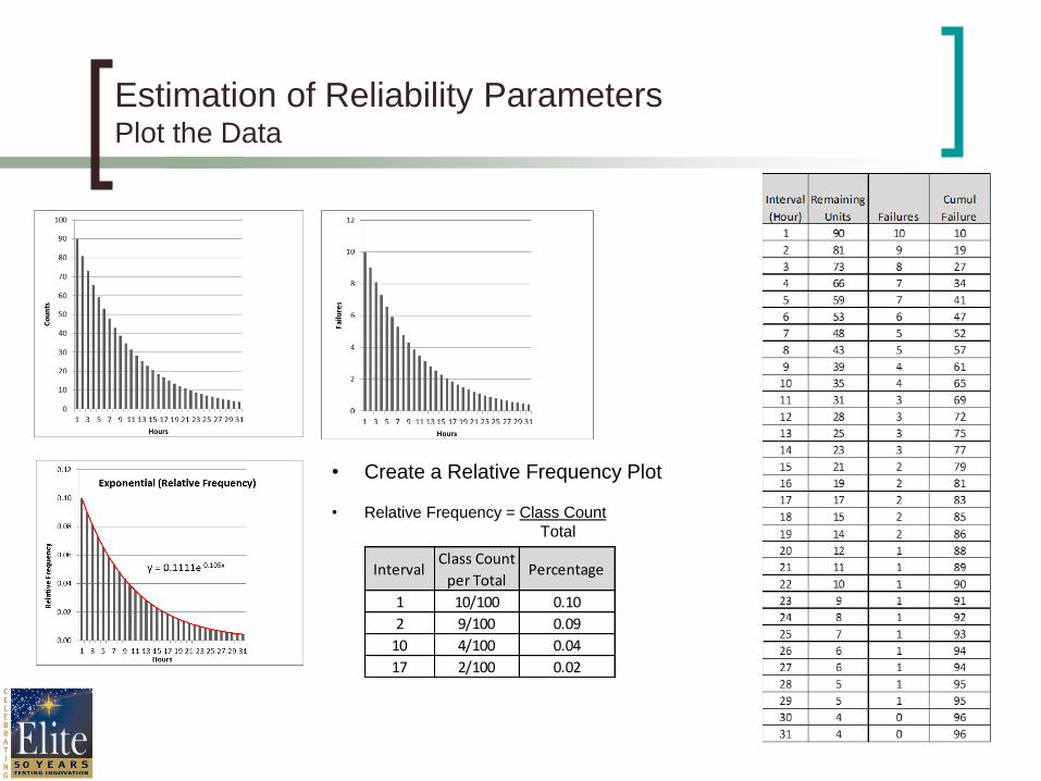
Estimation of Reliability Parameters Plot the Data
• Create a Relative Frequency Plot
• Relative Frequency = Class Count
Total • Evaluate the shape of the distribution
IntervalClass Count
per TotalPercentage
1 10/100 0.10
2 9/100 0.09
10 4/100 0.04
17 2/100 0.02

Estimation of Reliability Parameters
Probability Density Function (PDF)
• Relative likelihood for the variable to take on a given value.
• The probability density function is nonnegative everywhere,
and its integral over the entire space is equal to one
• Ex1:
• N=100
• = 0.1
• Evaluate at 10 hours
• f(10)= 0.036
• Ex2:
• N=100
• = 0.1
• Evaluate at 20 hours
• f(20)= 0.0135

Probability Density Functions (PDFs) to
Cumulative Distribution Functions (CDFs)
• Sum the area beneath the PDF
• CDF provides a probability of failure relative to x-
axis (time, cycles, life)
• The compliment of the CDF is the Reliability
Function.
• Reliability (x) = 1-CDF(x)
Reliability
Expression for
Exponential
Distribution Where
= failure rate
1/ = MTTF

Evaluate the Reliability Function
• Ex1:
• N=100
• = 0.1
• Evaluate at 10 hours
• R(10)= 0.36
• Ex2:
• N=100
• = 0.1
• Evaluate at 20 hours
• R(20)= 0. 135
Customer Provided Reliability Metrics
• = 1/MTTF
• Failure rate = 0.1
• MTTF = 10
Examples

Reliability Point Estimates and Confidence
• Calculate Confidence Intervals for Different Distributions
• Range of values bounded above and below within
which the true value is expected to fall.
• Measures the statistical precision of the estimate
• 90% confidence interval should contain the estimate
90% of the time
• Determine the interval within which the true
parametric values lies with a given probability for a
given sample size
• Determine the sample size required to assure with a
specified probability that the true parametric value
lies within a specific interval.
Exponential: Chi-Squared distribution
Normal: t-distribution
Weibull: See referenced resources…

Reliability Point Estimates and Confidence
Calculate Confidence Intervals
Exponential requires Chi-Squared Distribution
(Normal requires t-Distribution)
t* = time at which the life test is terminated
r = number of failures accumulated at time t*
T = total test time
a = acceptable risk of error
1 - a = confidence level
T = total test time
Note: Ref: 2
MTTF= 216hrs
115hrs 459hrs

Point Estimate for MTTF with Confidence Intervals
Example: Calculate MTTF with Confidence Intervals for Fixed
Truncation Time on 100 units, C=90%
n = number of items placed on test at time t = 0
t* = time at which the life test is terminated
r = number of failures accumulated at time t*
r* = preassigned number of failures
a = acceptable risk of error
1 - a = confidence level
T = total test time
Fixed Truncated Test
Lower One
Sided
Confidence
Bound
Two Sided
Confidence
Bound
= 1-CL
= 1-0.9 = 0.1
/2 = 0.05
r = 96
2r+2 = 194
2T c2(0.1, 194)
2T c2(0.05, 194)
2T c2(0.95, 192)
Lower One Sided Confidence Bound
Two Sided
Confidence
Bound
MTTF = 866 =9.02 hrs Total Test Time
96 Number of Failures
1732
219.633 (7.89, )
1732
227.496
1732
160.944
(7.61, 10.76)
Interval
(Hour)
Remain
Units Failures
Cumul
Failure
Cumul
Time
1 90 10 10 90
2 81 9 19 171
3 73 8 27 244
4 66 7 34 310
5 59 7 41 369
6 53 6 47 422
7 48 5 52 470
8 43 5 57 513
9 39 4 61 551
10 35 4 65 586
11 31 3 69 618
12 28 3 72 646
13 25 3 75 671
14 23 3 77 694
15 21 2 79 715
16 19 2 81 733
17 17 2 83 750
18 15 2 85 765
19 14 2 86 778
20 12 1 88 791
21 11 1 89 802
22 10 1 90 811
23 9 1 91 820
24 8 1 92 828
25 7 1 93 835
26 6 1 94 842
27 6 1 94 848
28 5 1 95 853
29 5 1 95 858
30 4 0 96 862
31 4 0 96 866
2T 1732

Chi Square Distribution Table
160.944 =CHIINV(0.95,20)
DF 0.995 0.975 0.2 0.1 0.05 0.025 0.02 0.01 0.005 0.002 0.001
190 143.545 153.721 206.182 215.371 223.16 230.064 232.146 238.266 243.959 250.977 255.976
191 144.413 154.621 207.225 216.437 224.245 231.165 233.251 239.386 245.091 252.124 257.135
192 145.282 155.521 208.268 217.502 225.329 232.265 234.356 240.505 246.223 253.271 258.292
193 146.15 156.421 209.311 218.568 226.413 233.365 235.461 241.623 247.354 254.418 259.45
194 147.02 157.321 210.354 219.633 227.496 234.465 236.566 242.742 248.485 255.564 260.607
195 147.889 158.221 211.397 220.698 228.58 235.564 237.67 243.86 249.616 256.71 261.763
196 148.759 159.122 212.439 221.763 229.663 236.664 238.774 244.977 250.746 257.855 262.92
197 149.629 160.023 213.482 222.828 230.746 237.763 239.877 246.095 251.876 259.001 264.075
198 150.499 160.925 214.524 223.892 231.829 238.861 240.981 247.212 253.006 260.145 265.231
199 151.37 161.826 215.567 224.957 232.912 239.96 242.084 248.329 254.135 261.29 266.386
200 152.241 162.728 216.609 226.021 233.994 241.058 243.187 249.445 255.264 262.434 267.541
201 153.112 163.63 217.651 227.085 235.077 242.156 244.29 250.561 256.393 263.578 268.695
202 153.984 164.532 218.693 228.149 236.159 243.254 245.392 251.677 257.521 264.721 269.849
203 154.856 165.435 219.735 229.213 237.24 244.351 246.494 252.793 258.649 265.864 271.002
204 155.728 166.338 220.777 230.276 238.322 245.448 247.596 253.908 259.777 267.007 272.155
205 156.601 167.241 221.818 231.34 239.403 246.545 248.698 255.023 260.904 268.149 273.308
P

Point Estimates for Reliability at Specified Time
with Confidence Intervals
• N=100
• = 0.1
• Evaluate at 10 hours
• R(10)= 0.36
Example
Fixed Truncated Test
Lower One
Sided
Confidence
Bound
Two Sided
Confidence
Bound7.61 10.758
R(10) =
R(10) = 0.268 0.395
2(866) c
2(0.95,192)
2(866) c
2(0.05,194)
2(866) 227.496
2(866) 160.994
Reliability
Expression for
Exponential
Distribution
Evaluate at 10 hours
R(10)= 0.36
2-sided 90% Confidence Intervals

Point Estimate for MTTF with Confidence Intervals
Example: Calculate MTTF with Confidence Intervals for Fixed
Number of Failures on 10 units, C=90%
n = number of items placed on test at time t = 0
t* = time at which the life test is terminated
r = number of failures accumulated at time t*
r* = preassigned number of failures
a = acceptable risk of error
1 - a = confidence level
T = total test time
= 1-CL
= 1-0.9 = 0.1
/2 = 0.05
r = 10
2r = 20
2T c2(0.1, 20)
2T c2(0.05, 20)
2T c2(0.95, 20)
Lower One Sided Confidence Bound
Two Sided
Confidence
Bound
MTTF = 961 =96.1 hrs Total Test Time
10 Number of Failures
Failure
Number
Operating
Time (Hrs)
1 8
2 20
3 34
4 46
5 63
6 86
7 111
8 141
9 186
10 266
Total 961
2T 1922
1922
28.412 (67.6, )
1922
31.41
1922
10.851
(61.19, 177.12)
Fixed Number of Failures
Lower One
Sided
Confidence
Interval
Two Sided
Confidence
Interval

Chi Square Distribution Table
10.85081 =CHIINV(0.95,20)
DF 0.995 0.975 0.2 0.1 0.05 0.025 0.02 0.01 0.005 0.002 0.001
1 3.93E-05 0.000982 1.642 2.706 3.841 5.024 5.412 6.635 7.879 9.55 10.828
2 0.01 0.0506 3.219 4.605 5.991 7.378 7.824 9.21 10.597 12.429 13.816
3 0.0717 0.216 4.642 6.251 7.815 9.348 9.837 11.345 12.838 14.796 16.266
4 0.207 0.484 5.989 7.779 9.488 11.143 11.668 13.277 14.86 16.924 18.467
5 0.412 0.831 7.289 9.236 11.07 12.833 13.388 15.086 16.75 18.907 20.515
6 0.676 1.237 8.558 10.645 12.592 14.449 15.033 16.812 18.548 20.791 22.458
7 0.989 1.69 9.803 12.017 14.067 16.013 16.622 18.475 20.278 22.601 24.322
8 1.344 2.18 11.03 13.362 15.507 17.535 18.168 20.09 21.955 24.352 26.124
9 1.735 2.7 12.242 14.684 16.919 19.023 19.679 21.666 23.589 26.056 27.877
10 2.156 3.247 13.442 15.987 18.307 20.483 21.161 23.209 25.188 27.722 29.588
11 2.603 3.816 14.631 17.275 19.675 21.92 22.618 24.725 26.757 29.354 31.264
12 3.074 4.404 15.812 18.549 21.026 23.337 24.054 26.217 28.3 30.957 32.909
13 3.565 5.009 16.985 19.812 22.362 24.736 25.472 27.688 29.819 32.535 34.528
14 4.075 5.629 18.151 21.064 23.685 26.119 26.873 29.141 31.319 34.091 36.123
15 4.601 6.262 19.311 22.307 24.996 27.488 28.259 30.578 32.801 35.628 37.697
16 5.142 6.908 20.465 23.542 26.296 28.845 29.633 32 34.267 37.146 39.252
17 5.697 7.564 21.615 24.769 27.587 30.191 30.995 33.409 35.718 38.648 40.79
18 6.265 8.231 22.76 25.989 28.869 31.526 32.346 34.805 37.156 40.136 42.312
19 6.844 8.907 23.9 27.204 30.144 32.852 33.687 36.191 38.582 41.61 43.82
20 7.434 9.591 25.038 28.412 31.41 34.17 35.02 37.566 39.997 43.072 45.315
21 8.034 10.283 26.171 29.615 32.671 35.479 36.343 38.932 41.401 44.522 46.797
22 8.643 10.982 27.301 30.813 33.924 36.781 37.659 40.289 42.796 45.962 48.268
23 9.26 11.689 28.429 32.007 35.172 38.076 38.968 41.638 44.181 47.391 49.728
24 9.886 12.401 29.553 33.196 36.415 39.364 40.27 42.98 45.559 48.812 51.179
25 10.52 13.12 30.675 34.382 37.652 40.646 41.566 44.314 46.928 50.223 52.62
P

Procedure for Calculating Point Estimates
and Confidence Intervals
IEC 60505-4 Statistical Procedures for
Exponential Distribution-
Point Estimates,
Confidence Intervals,
Prediction Intervals and
Tolerance Intervals

IEC Tools For Reliability Assessment
IEC 60300-3-5 Reliability Test Conditions and
Statistical Test Principles
IEC 11453 Point Estimate and Confidence
Intervals for the Binominal
Distribution
IEC 60605-4 Point Estimate and Confidence
Intervals for the Exponential
Distribution
IEC 11453
IEC 60605-4
IEC 61649 Point Estimate and Confidence
Intervals for the Weibull Distribution
IEC 61649 IEC 61164
IEC 60605-6

Important Distributions
Exponential • Constant Failure Rate
• Mixed Failure Modes
• Most Electronics
• Mean Life R(t)= 0.368
Normal • Wear-out
• Greater than 20 samples
• Mean Life R(t)= 0.5
Weibull • Can model a variety of
different data types
• Infant mortality, constant
failure rate, or wear-out.
• Good for limited samples

Weibull Analysis
Method for representing and interpreting data
Provides a Reliability metric directly from plot
Works well with small samples – life data
(failures) provide more information
(shape or slope), (characteristic life or scale),
(location or offset)
< 1 indicates infant mortality
= 1 indicates random failures
> 1 indicates wear out failures

Weibull Analysis
1. Acquire accurate time to failure data
2. Rank the data first failure to last
3. Plot the data on Weibull paper
4. Interpret the plot 1. Look for mixed modes
2. Measure slope to determine
3. Determine characteristic life
4. Read R(t)
Failure
Number
Operating
Time
(Hours)
Median
Rank 10
Samples
1 8 6.70
2 20 16.23
3 34 25.86
4 46 35.51
5 63 45.17
6 86 54.83
7 111 64.49
8 141 74.14
9 186 83.77
10 266 93.30
Rank Order 1 2 3 4 5 6 7 8 9 10
1 50.00 29.29 20.63 15.91 12.94 10.91 9.43 8.30 7.41 6.70
2 70.71 50.00 38.57 31.38 26.44 22.85 20.11 17.96 16.23
3 79.37 61.43 50.00 42.14 36.41 32.05 28.62 25.86
4 84.09 68.62 57.86 50.00 44.02 39.31 35.51
5 87.06 73.56 63.59 55.98 50.00 45.17
6 89.09 77.15 67.95 60.69 54.83
7 90.57 79.89 71.38 64.49
8 91.70 82.04 74.14
9 92.59 83.77
10 93.30
Sample Size
Median Rank Table
Median Rank Estimate
MR = (i-0.3) *100
(N+0.4)
i= rank order #
N=sample size

MTTF vs. MTBF
MTTF- Mean Time To Failure
Expected time to fail for a non-repairable system
Non-repairable systems can fail only once.
MTTF is equivalent to the mean of its failure time distribution.
Ex 16+12+14+6+8 = 56/5= 11.2
MTBF- Mean Time Between Failure
Expected time to fail for repairable systems
Expected time between two consecutive failures for a repairable system
MTBF= MTTF +MTTR
16hrs 12hrs 14hrs 6hrs 8hrs
Re
pai
r/R
est
ore
Re
pai
r/R
est
ore
Re
pai
r/R
est
ore
Re
pai
r/R
est
ore
Re
pai
r/R
est
ore
Re
pai
r/R
est
ore
Operational
Non-Operational
Time Between Failures
Repair Time
12hrs
16hrs
6hrs
14hrs
8hrs
StartFailure

100
20
Interval
(Hour)
Remaining
Units
(Exp)
Failures
(Exp)
Cumul
Failure
(Exp)
Cumul
Time
(Exp)
Failure
Rate
(Exp)
Rel Freq
(Exp)
1 80 20 20 80 0.20 0.20
2 64 16 36 144 0.20 0.16
3 51 13 49 195 0.20 0.13
4 41 10 59 236 0.20 0.10
5 33 8 67 269 0.20 0.08
6 26 7 74 295 0.20 0.07
7 21 5 79 316 0.20 0.05
8 17 4 83 333 0.20 0.04
9 13 3 87 346 0.20 0.03
10 11 3 89 357 0.20 0.03
11 9 2 91 366 0.20 0.02
12 7 2 93 373 0.20 0.02
13 5 1 95 378 0.20 0.01
14 4 1 96 382 0.20 0.01
15 4 1 96 386 0.20 0.01
16 3 1 97 389 0.20 0.01
17 2 1 98 391 0.20 0.01
18 2 0 98 393 0.20 0.00
19 1 0 99 394 0.20 0.00
20 1 0 99 395 0.20 0.00
21 1 0 99 396 0.20 0.00
22 1 0 99 397 0.20 0.00
23 1 0 99 398 0.20 0.00
24 0 0 100 398 0.20 0.00
25 0 0 100 398 0.20 0.00
26 0 0 100 399 0.20 0.00
27 0 0 100 399 0.20 0.00
28 0 0 100 399 0.20 0.00
29 0 0 100 399 0.20 0.00
30 0 0 100 400 0.20 0.00
31 0 0 100 400 0.20 0.00
Total 1.0
400 Lower Single-Sided Confidence Limit at 90%
100
0
90
0.1
199.80 4.0
100
227.09
235.08
167.36
Total Qty At Start of Test
% Failure Rate (Exponential)
4.8
Total Accumulated Test Time (T)
Number of Failures
Number of Suspensions
Confidence Limit
Alpha
2r
Lower 2-Sided Confidence Limit at
90 %
Upper 2-Sided Confidence Limit at
90%MTTF
r
Lower Single-Sided
Lower 2-Sided
Upper 2-Sided
3.5
3.4
0
10
20
30
40
50
60
70
80
90
1 3 5 7 9 11 13 15 17 19 21 23 25 27 29 31
Co
un
ts
Hours
Exponential
y = 0.25e-0.223x
0.00
0.05
0.10
0.15
0.20
0.25
1 3 5 7 9 11 13 15 17 19 21 23 25 27 29 31
Re
lati
ve F
req
ue
ncy
Hours
Exponential (Relative Frequency)
y = 0.2e-0.2x
0
0.02
0.04
0.06
0.08
0.1
0.12
0.14
0.16
0.18
0 10 20 30
Pro
bab
ility
De
nsi
ty
Hours
Exponential PDF
-0.2
0
0.2
0.4
0.6
0.8
1
1.2
0 5 10 15 20 25 30
Cu
mu
lati
ve D
en
sity
Fu
nct
ion
Re
liab
ility
Fu
nct
ion
Exponential CDF & Reliability Function

Reliability Bathtub Curve
Exponential Distribution
= failure rate = constant
Weibull Distribution
< 1 indicates infant mortality
= 1 indicates random failures
> 1 indicates wear out failures

System Reliability
Rsystem = Rsubsystem1 *Rsubsystem2 *Rsubsystem3… *Ri
Block Diagrams
Series
Parallel-Series
.97
.93 .98 .95 R System = 0.84
.97 .93
.93
.98 .95 R System = 0.90

Success Run Test to Establish R & C
Success Run Test, Test to a Bogey
Based on a Binomial Distribution
Test Results are Either Success or Failure
Prove a Target Reliability with an assigned Confidence Level
Don’t care about continuous measurement or calculating a parametric value, ie
MTTF or failure rate
Define the test conditions to represent 1 or more lives
Operate without failure for a specified time
Reliability, Confidence, and Sample Size related by Success Run Formula N= Sample Size, R= Reliability, C= Confidence Level

Success Run Test to Establish R & C
Calculate required number of samples based on R and C
Example
R= 97%, C= 50%
Example
R= 97.7%, C= 90%

Binomial Distribution
Nomograph for
R/C/N
HALT/HASS and Accelerated Testing
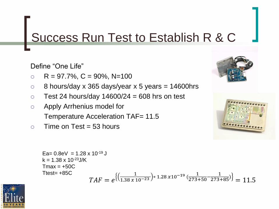
Success Run Test to Establish R & C
Define “One Life”
R = 97.7%, C = 90%, N=100
8 hours/day x 365 days/year x 5 years = 14600hrs
Test 24 hours/day 14600/24 = 608 hrs on test
Apply Arrhenius model for
Temperature Acceleration TAF= 11.5
Time on Test = 53 hours
Ea= 0.8eV = 1.28 x 10⁻¹⁹ J
k = 1.38 x 10⁻²³J/K
Tmax = +50C
Ttest= +85C

Time Dependent Failure Mechanisms
Loss of signal Silicon Diffusion Temperature
Power Failure Dielectric Breakdown Electric Field
Loss of signal Electromigration Temperature & Power Cycling
Intermittent Output Corrosion & Oxidation of Fractures Humidity, Voltage, Temperature
Loss of signal Dendrite Growth Humidity, Temperature
Water Intrusion Seal Leaks Pressure
Cracked Solder Joint Fatigue Thermal cycling & vibration
Failure Mechanism Accelerating Factors Failure Mode
Overstress- ESD, Mechanical Shock, Thermal Breakdown
Time Dependent- Fatigue, Wear, Corrosion

Accelerated Stress Testing
Acceleration Factors
o Temperature
o Arrhenius Model
o Humidity
o Lawson Model
o Coffin-Manson
o Vibration
o Power Law and Miner
Criteria m= S-N slope
o Voltage
o Inverse Power Law
o Product Life Cycling o CALT Testing
o Test to Failure & Apply
Weibull Analysis

MIL-HDBK-338 Table 8-7.1

Product Life Cycling
Calibrated Accelerated Life Testing (CALT)
Suggest primary fatigue mechanism
Simulate loads at three stress levels
90% of foolish load (first test)
80% of first test load
Third stress level
Depends on first two and ultimate life
Test all units to failure
Plot S-N curve, Determine AF’s
Generate Weibull Plot
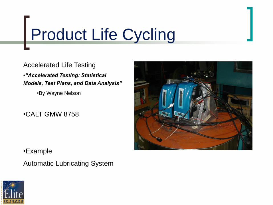
Product Life Cycling
Accelerated Life Testing
•“Accelerated Testing: Statistical
Models, Test Plans, and Data Analysis”
•By Wayne Nelson
•CALT GMW 8758
•Example
Automatic Lubricating System

CALT Test Example
•Simulate loads
at three stress
levels
•Monitor test
counting cycles
to failure

CALT Test Example Stress Cycles To Failure
36 3121
36 1075
36 629
36 9452
31 11386
31 1104
31 6624
31 1577
25 11044
25 15405
25 19257
25 28723
Pump S-N Curve
y = 3050953219559.39x-5.93
100
1000
10000
100000
10 100Applied Stress (PSI)C
ycle
s t
o F
ailu
re
•Collect Failure Data
•Plot and determine Inverse
Power Relationship
•AF = (Saccel/Snormal)b
Determine AF's
Condition
High Stress
Mid Stress
Confirm Stress
Normal Stress
Accel Factor
180
74
21
Stress Value (PSI)
36
31
25
15 N/A
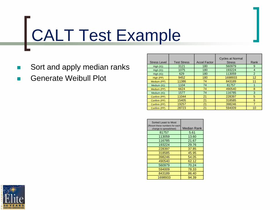
CALT Test Example
Stress Level Test Stress Accel Factor Rank
High (IG) 3121 180 9
High (IG) 1075 180 4
High (IG) 629 180 2
High (PP) 9452 180 12
Medium (PP) 11386 74 11
Medium (IG) 1104 74 1
Medium (PP) 6624 74 8
Medium (IG) 1577 74 3
Confirm (PP) 11044 21 5
Confirm (PP) 15405 21 6
Confirm (PP) 19257 21 7
Confirm (PP) 28723 21 10
Cycles at Normal
Stress
560979
193224
113059
1698933
398246
594009
843189
81757
490540
116785
228397
318585
Median Rank
5.61
13.60
21.67
29.76
37.85
45.95
54.05
62.12
70.24
78.33
86.40
94.39
81757
228397
594009
843189
1698933
Sorted Least to Most (Resort these numbers for each
change to spreadsheet)
318585
398246
490540
560979
113059
116785
193224
Sort and apply median ranks
Generate Weibull Plot

HALT/HASS and Accelerated Testing
CALT Test Example
Weibull Plot
•Obtain distribution parameters
•Reliability metrics
•B1, B10
•Reliability vs life

Vibration Testing Techniques
Servo-Hydraulic Electro-Dynamic Repetitive Shock
• Frequency Range 3Hz-2,500Hz
• Programmable vibration
characteristics; Sine, Random, Sine-on-
Random, Random-on-Random, Field
Data Replay, Mechanical Shock
• Displacement generally limited to 2-3” p-p
• Single axis motion
• Frequency Range 0.5Hz-300Hz
• Programmable vibration
characteristics; Sine, Random, Sine-
on-Random, Random-on-Random, Field
Data Replay, Mechanical Shock
• Displacement generally up to 12” p-p
• Multi-axis motion from multiple cylinders
• Frequency Range 20Hz-10,00Hz
• Vibration output quasi-random with
limited PSD shaping
• Six-axis simultaneous vibration
• High G peak levels • Displacement generally limited to 0.5”

Electro-Dynamic Vibration Machine
Armature Field coil Field
Current
Thrust
Armature
Center Pole Base
Body
Thermotron armature and
cut-away illustration here???

Vibration Time & Frequency Domain
G2/Hz
0.1
Hz
G pk
2
Hz50
1
2
Hz100
1G pk
Power
Spectral
Density
(PSD)
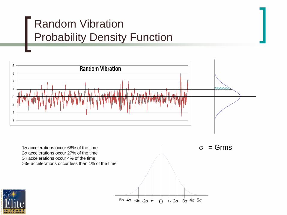
Random Vibration
Probability Density Function
o 2 3 -2 - -3 -4 -5 4 5
1 accelerations occur 68% of the time
2 accelerations occur 27% of the time
3 accelerations occur 4% of the time
>3 accelerations occur less than 1% of the time
= Grms

Random Vibration
Power Spectral Density Plots
Which is the more severe test?
G2/HzG2/Hz
G2/Hz
0.1 0.1 0.1
0.2 0.2 0.2 0.2 0.20.2 0.2 0.2 0.2
Hz Hz Hz

Power Spectral Density Plots

Vibration Testing
Vibration fatigue failures are caused by stress reversals
Vibration at resonance amplifies damage
High accelerations generate proportional Displacements,
Velocities, and Forces, and damage
A higher concentration of High G peak accelerations has the
potential for greater damage
Most ED vibration testing limits peak accelerations to 3-sigma
RS vibration generates a greater proportion of High G peak
accelerations
HALT/HASS and Accelerated Testing

Which Tests To Run
Input from all departments
Determine failure modes (FMEA)
Consider complete life cycle of product
Suggest stresses that will precipitate failures Maximum Stress vs Time Dependent
Develop test plan
Execute test

Failure of Electronic Equipment
20 year U.S. Air Force Study
55% of failures due to high temperature and thermal
cycling
20% of failures due to vibration and shock
20% due to humidity

New Product Development Testing Screens
Qualitative Testing
Qualification
Testing Qual Retest
Quantitative Testing Manufacturing
Screen
New
Product
HALT, HAST, ESD,
Power Cycle, EMI RTCA DO-160
MIL-810,
SAE J1455
Temp, Vibration, Shock,
Waterproofness,
Altitude, Humidity
HASS Analysis
Phase
Development
Phase

Essential Reliability Reference Documents
Vibration Analysis For Electronic Equipment, David S. Steinberg, Third Edition
MIL-HDBK-338B Oct 1998 Military Handbook- Electronic Reliability Design Handbook
The New Weibull Handbook, R.B. Abernathy
Practical Reliability Engineering, Patrick O'Connor
IEC 60300-3-5 Reliability Test Conditions and Statistical Test Principles
GMW 3172:2010
HALT/HASS and Accelerated Testing

HALT and Relaibility Workshop
Any Questions?
Thank You!