Hadoop­GIS: A High Performance Spatial DataWarehousing System over MapReduce

Ablimit Aji1 Fusheng Wang2 Hoang Vo1 Rubao Lee3 Qiaoling Liu1 Xiaodong Zhang3 Joel Saltz2

1Department of Mathematics and Computer Science, Emory University2Department of Biomedical Informatics, Emory University

3Department of Computer Science and Engineering, The Ohio State University

ABSTRACTSupport of high performance queries on large volumes of spatialdata becomes increasingly important in many application domains,including geospatial problems in numerous fields, location basedservices, and emerging scientific applications that are increasinglydata- and compute-intensive. The emergence of massive scale spa-tial data is due to the proliferation of cost effective and ubiquitouspositioning technologies, development of high resolution imagingtechnologies, and contribution from a large number of communityusers. There are two major challenges for managing and queryingmassive spatial data to support spatial queries: the explosion of spa-tial data, and the high computational complexity of spatial queries.In this paper, we present Hadoop-GIS – a scalable and high per-formance spatial data warehousing system for running large scalespatial queries on Hadoop. Hadoop-GIS supports multiple typesof spatial queries on MapReduce through spatial partitioning, cus-tomizable spatial query engine RESQUE, implicit parallel spatialquery execution on MapReduce, and effective methods for amend-ing query results through handling boundary objects. Hadoop-GISutilizes global partition indexing and customizable on demand localspatial indexing to achieve efficient query processing. Hadoop-GISis integrated into Hive to support declarative spatial queries withan integrated architecture. Our experiments have demonstrated thehigh efficiency of Hadoop-GIS on query response and high scal-ability to run on commodity clusters. Our comparative experi-ments have showed that performance of Hadoop-GIS is on par withparallel SDBMS and outperforms SDBMS for compute-intensivequeries. Hadoop-GIS is available as a set of library for processingspatial queries, and as an integrated software package in Hive.

1. INTRODUCTIONThe proliferation of cost effective and ubiquitous positioning

technologies has enabled capturing spatially oriented data at an un-precedented scale and rate. Collaborative spatial data collection ef-forts, such as OpenStreetMap [8], further accelerate the generationof massive spatial information from community users. Analyzinglarge amounts of spatial data to derive values and guide decisionmaking have become essential to business success and scientific

Permission to make digital or hard copies of all or part of this work forpersonal or classroom use is granted without fee provided that copies arenot made or distributed for profit or commercial advantage and that copiesbear this notice and the full citation on the first page. To copy otherwise, torepublish, to post on servers or to redistribute to lists, requires prior specificpermission and/or a fee. Articles from this volume were invited to presenttheir results at The 39th International Conference on Very Large Data Bases,August 26th ­ 30th 2013, Riva del Garda, Trento, Italy.Proceedings of the VLDB Endowment, Vol. 6, No. 11Copyright 2013 VLDB Endowment 2150­8097/13/09... $ 10.00.

discoveries. For example, Location Based Social Networks (LB-SNs) are utilizing large amounts of user location information toprovide geo-marketing and recommendation services. Social sci-entists are relying on such data to study dynamics of social systemsand understand human behavior.

The rapid growth of spatial data is driven by not only industrialapplications, but also emerging scientific applications that are in-creasingly data- and compute- intensive. With the rapid improve-ment of data acquisition technologies such as high-resolution tis-sue slide scanners and remote sensing instruments, it has becomemore efficient to capture extremely large spatial data to supportscientific research. For example, digital pathology imaging hasbecome an emerging field in the past decade, where examinationof high resolution images of tissue specimens enables novel, moreeffective ways of screening for disease, classifying disease states,understanding disease progression and evaluating the efficacy oftherapeutic strategies. Pathology image analysis offers a meansof rapidly carrying out quantitative, reproducible measurements ofmicro-anatomical features in high-resolution pathology images andlarge image datasets. Regions of micro-anatomic objects (millionsper image) such as nuclei and cells are computed through imagesegmentation algorithms, represented with their boundaries, andimage features are extracted from these objects. Exploring theresults of such analysis involves complex queries such as spatialcross-matching, overlay of multiple sets of spatial objects, spatialproximity computations between objects, and queries for globalspatial pattern discovery. These queries often involve billions ofspatial objects and heavy geometric computations.

A major requirement for the data intensive spatial applicationsis fast query response which requires a scalable architecture thatcan query spatial data on a large scale. Another requirement is tosupport queries on a cost effective architecture such as commodityclusters or cloud environments. Meanwhile, scientific researchersand application developers often prefer expressive query languagesor interfaces to express complex queries with ease, without worry-ing about how queries are translated, optimized and executed. Withthe rapid improvement of instrument resolutions, increased accu-racy of data analysis methods, and the massive scale of observeddata, complex spatial queries have become increasingly compute-and data-intensive due to following challenges.

The Big Data Challenge. High resolution microscopy imagesfrom high resolution digital slide scanners provide rich informa-tion about spatial objects and their associated features. For ex-ample, whole-slide images (WSI) made by scanning microscopeslides at diagnostic resolution are very large: A typical WSI con-tains 100,000x100,000 pixels. One image may contain millions ofobjects, and hundreds of image features can be extracted for eachobject. A study may involve hundreds or thousands of images ob-

1009

tained from a large cohort of subjects. For large scale interrelatedanalysis, there may be dozens of algorithms - with varying parame-ters - to generate many different result sets to be compared and con-solidated. Thus, derived data from images of a single study is oftenin the scale of tens of terabytes. A moderate-size hospital can rou-tinely generate thousands of whole slide images per day, which canlead to several terabytes of derived analytical results per day, andpetabytes of data can be easily created within a year. For the Open-StreetMap project, there have been more than 600,000 registeredcontributors, and user contributed data is increasing continuously.

High Computation Complexity. Most spatial queries involve ge-ometric computations which are often compute-intensive. Geomet-ric computation is not only used for computing measurements orgenerating new spatial objects, but also as logical operations fortopology relationships. While spatial filtering through minimumbounding rectangles (MBRs) can be accelerated through spatial ac-cess methods, spatial refinements such as polygon intersection ver-ification are highly expensive operations. For example, spatial joinqueries such as spatial cross-matching or overlaying multiple setsof spatial objects on an image or map can be very expensive toprocess.

The large amounts of data coupled with compute-intensive na-ture of spatial queries require a scalable and efficient solution. Apotential approach for scaling out spatial queries is through a paral-lel DBMS. In the past, we have developed and deployed a parallelspatial database solution – PAIS [35, 34, 9]. However, this approachis highly expensive on software licensing and dedicated hardware,and requires sophisticated tuning and maintenance efforts [29].

Recently, MapReduce based systems have emerged as a scalableand cost effective solution for massively parallel data processing.Hadoop, the open source implementation of MapReduce, has beensuccessfully applied in large scale internet services to support bigdata analytics. Declarative query interfaces such as Hive [32], Pig[21], and Scope [19] have brought the large scale data analysis onestep closer to the common users by providing high level, easy touse programming abstractions to MapReduce. In practice, Hive iswidely adopted as a scalable data warehousing solution in manyenterprises, including Facebook. Recently we have developed asystem YSmart [24], a correlation aware SQL to MapReduce trans-lator for optimized queries, and have integrated it into Hive.

However, most of these MapReduce based systems either lackspatial query processing capabilities or have limited spatial querysupport. While the MapReduce model fits nicely with large scaleproblems through key-based partitioning, spatial queries and an-alytics are intrinsically complex and difficult to fit into the modeldue to its multi-dimensional nature [11]. There are two major prob-lems to handle for spatial partitioning: spatial data skew problemand boundary object problem. The first problem could lead to loadimbalance of tasks in distributed systems and long response time,and the second problem could lead to incorrect query results if nothandled properly. In addition, spatial query methods have to beadapted so that they can be mapped into partition based query pro-cessing framework while preserving the correct query semantics.Spatial queries are also intrinsically complex which often rely oneffective access methods to reduce search space and alleviate highcost of geometric computations. Thus, there is a significant steprequired on adapting and redesigning spatial query methods to takeadvantage of the MapReduce computing infrastructure.

We have developed Hadoop-GIS [7] – a spatial data warehous-ing system over MapReduce. The goal of the system is to delivera scalable, efficient, expressive spatial querying system to supportanalytical queries on large scale spatial data, and to provide a fea-sible solution that can be afforded for daily operations. Hadoop-

GIS provides a framework on parallelizing multiple types of spa-tial queries and having the query pipelines mapped onto MapRe-duce. Hadoop-GIS provides spatial data partitioning to achievetask parallelization, an indexing-driven spatial query engine to pro-cess various types of spatial queries, implicit query parallelizationthrough MapReduce, and boundary handling to generate correctresults. By integrating the framework with Hive, Hadoop-GIS pro-vides an expressive spatial query language by extending HiveQL[33] with spatial constructs, and automates spatial query translationand execution. Hadoop-GIS supports fundamental spatial queriessuch as point, containment, join, and complex queries such as spa-tial cross-matching (large scale spatial join) and nearest neighborqueries. Structured feature queries are also supported through Hiveand fully integrated with spatial queries.

The rest of the paper is organized as follows. We first presentan architectural overview of Hadoop-GIS in Section 2. The spatialquery engine is discussed in Section 3, MapReduce based spatialquery processing is presented in Section 4, boundary object han-dling for spatial queries is discussed in Section 5, integration ofspatial queries into Hive is discussed in Section 6, performancestudy is discussed in Section 7, which followed by related workand conclusion.

2. OVERVIEW

2.1 Query CasesThere are five major categories of queries: i) feature aggregation

queries (non-spatial queries), for example, queries for finding meanvalues of attributes or distribution of attributes; ii) fundamental spa-tial queries, including point based queries, containment queries andspatial joins; iii) complex spatial queries, including spatial cross-matching or overlay (large scale spatial join) and nearest neighborqueries; iv) integrated spatial and feature queries, for example, fea-ture aggregation queries in a selected spatial regions; and v) globalspatial pattern queries, for example, queries on finding high den-sity regions, or queries to find directional patterns of spatial ob-jects. In this paper, we mainly focus on a subset of cost-intensivequeries which are commonly used in spatial warehousing appli-cations. Support of multiway join queries and nearest neighborqueries are discussed in our previous work [12], and we are plan-ning to study global spatial pattern queries in our future work.

In particular, spatial cross-matching/overlay problem involvesidentifying and comparing objects belonging to different observa-tions or analyses. Cross-matching in the domain of sky survey aimsat performing one-to-one matches in order to combine physicalproperties or study the temporal evolution of the source [26]. Herespatial cross-matching refers to finding spatial objects that overlapor intersect each other [36]. For example, in pathology imaging,spatial cross-matching is often used to compare and evaluate imagesegmentation algorithm results, iteratively develop high quality im-age analysis algorithms, and consolidate multiple analysis resultsfrom different approaches to generate more confident results. Spa-tial cross-matching can also support spatial overlays for combininginformation for massive spatial objects between multiple layers orsources of spatial data, such as remote sensing datasets from dif-ferent satellites. Spatial cross-matching can also be used to findtemporal changes of maps between time snapshots.

2.2 Traditional Methods for Spatial QueriesTraditional spatial database management systems (SDBMSs) have

been used for managing and querying spatial data, through ex-tended spatial capabilities on top of ORDBMS. These systems of-ten have major limitations on managing and querying spatial data

1010

at massive scale, although parallel RDBMS architectures [28] canbe used to achieve scalability. Parallel SDBMSs tend to reducethe I/O bottleneck through partitioning of data on multiple paral-lel disks and are not optimized for computationally intensive op-erations such as geometric computations. Furthermore, parallelSDBMS architecture often lacks effective spatial partitioning mech-anism to balance data and task loads across database partitions, anddoes not inherently support a way to handle boundary crossing ob-jects. The high data loading overhead is another major bottleneckfor SDBMS based solutions [29]. Our experiments show that load-ing the results from a single whole slide image into a SDBMS cantake a few minutes to dozens of minutes. Scaling out spatial queriesthrough a parallel database infrastructure is studied in our previouswork [34, 35], but the approach is highly expensive and requiressophisticated tuning for optimal performance.

2.3 Overview of MethodsThe main goal of Hadoop-GIS is to develop a highly scalable,

cost-effective, efficient and expressive integrated spatial query pro-cessing system for data- and compute-intensive spatial applications,that can take advantage of MapReduce running on commodity clus-ters. To realize such system, it is essential to identify time consum-ing spatial query components, break them down into small tasks,and process these tasks in parallel. An intuitive approach is to spa-tially partition the data into buckets (or tiles), and process thesebuckets in parallel. Thus, generated tiles will become the unit forquery processing. The query processing problem then becomes theproblem on designing querying methods that can run on these tilesindependently, while preserving the correct query semantics. InMapReduce environment, we propose the following steps on run-ning a typical spatial query, as shown in Algorithm 1.

In step A, we perform effective space partitioning to generatetiles. In step B, spatial objects are assigned tile UIDs, mergedand stored into HDFS. Step C is for pre-processing queries, whichcould be queries that perform global index based filtering, queriesthat do not need to run in tile based query processing framework.Step D performs tile based spatial query processing independently,which are parallelized through MapReduce. Step E provides han-dling of boundary objects (if needed), which can run as anotherMapReduce job. Step F does post-query processing, for example,joining spatial query results with feature tables, which could be an-other MapReduce job. Step G does data aggregation of final results,and final results are output into HDFS. Next we briefly discussthe architectural components of Hadoop-GIS (HiveSP ) as shown inFigure 1, including data partitioning, data storage, query languageand query translation, and query engine. The query engine consistsof index building, query processing and boundary handling on topof Hadoop.

2.4 Data PartitioningSpatial data partitioning is an essential initial step to define, gen-

erate and represent partitioned data. There are two major consid-erations for spatial data partitioning. The first consideration is toavoid high density partitioned tiles. This is mainly due to poten-tial high data skew in the spatial dataset, which could cause loadimbalance among workers in a cluster environment. Another con-sideration is to handle boundary intersecting objects properly. AsMapReduce provides its own job scheduling for balancing tasks,the load imbalance problem can be partially alleviated at the taskscheduling level. Therefore, for spatial data partitioning, we mainlyfocus on breaking high density tiles into smaller ones, and take arecursive partitioning approach. For boundary intersecting objects,we take the multiple assignment based approach in which objects

Algorithm 1: Typical workflow of spatial query processing onMapReduce

A. Data/space partitioning;B. Data storage of partitioned data on HDFS;C. Pre-query processing (optional);D. for tile in input collection do

Index building for objects in the tile;Tile based spatial querying processing;

E. Boundary object handling;F. Post-query processing (optional);G. Data aggregation;H. Result storage on HDFS;

Input Data Storage Querying System

RESQUE

Spatial Query

Processor

Spatial Index

Builder

QLSP Query Language

Spatial S

hapes

Featu

res

HadoopHDFS

Tile Spatial Indexes

Global Spatial Indexes

Boundary Handling

Web InterfaceCmd Line Interface

Da

ta P

art

itio

nin

g

QLSP Parser/Query Translator/Query Optimizer

Query Translation

Query Engine

Figure 1: Architecture overview of Hadoop-GIS (HiveSP )

are replicated and assigned to each intersecting tile, followed by apost-processing step for remedying query results (section 5).

2.5 Real­time Spatial Query EngineA fundamental component we aim to provide is a standalone spa-

tial query engine with such requirements: i) is generic enough tosupport a variety of spatial queries and can be extended; ii) canbe easily parallelized on clusters with decoupled spatial query pro-cessing and (implicit) parallelization; and iii) can leverage existingindexing and querying methods. Porting a spatial database enginefor such purpose is not feasible, due to its tight integration withRDBMS engine and complexity on setup and optimization. Wedevelop a Real-time Spatial Query Engine (RESQUE) to supportspatial query processing, as shown in the architecture in Figure 1.RESQUE takes advantage of global tile indexes and local indexescreated on demand to support efficient spatial queries. Besides,RESQUE is fully optimized, supports data compression, and comeswith very low overhead on data loading. This makes RESQUEa highly efficient spatial query engine compared to a traditionalSDBMS engine. RESQUE is compiled as a shared library whichcan be easily deployed in a cluster environment. Hadoop-GIS takesadvantage of spatial access methods for query processing with twoapproaches. At the higher level, Hadoop-GIS creates global re-gion based spatial indexes of partitioned tiles for HDFS file splitfiltering. As a result, for many spatial queries such as containmentqueries, we can efficiently filter most irrelevant tiles through thisglobal region index. The global region index is small and can bestored in a binary format in HDFS and shared across cluster nodesthrough Hadoop distributed cache mechanism. At the tile level,RESQUE supports an indexing on demand approach by buildingtile based spatial indexes on the fly, mainly for query processing

1011

purpose, and storing index files in the main memory. Since thetile size is relatively small, index building on a single tile is veryfast and it greatly enhances spatial query processing performance.Our experiments show that, with increasing speed of CPU, index-ing building overhead is a very small fraction of compute- and data-intensive spatial queries such as cross-matching.

2.6 MapReduce Based Parallel Query Execu­tion

Instead of using explicit spatial query parallelization as summa-rized in [17], we take an implicit parallelization approach by lever-aging MapReduce. This will much simplify the development andmanagement of query jobs on clusters. As data is spatially parti-tioned, the tile name or UID forms the key for MapReduce, andidentifying spatial objects of tiles can be performed in mappingphase. Depending on the query complexity, spatial queries canbe implemented as map functions, reduce functions or combina-tion of both. Based on the query types, different query pipelinesare executed in MapReduce. As many spatial queries involve highcomplexity geometric computations, query parallelization throughMapReduce can significantly reduce query response time.

2.7 Boundary Object HandlingIn the past, two approaches were proposed to handle boundary

objects in a parallel query processing scenario, namely MultipleAssignment and Multiple Matching [25, 40]. In multiple assign-ment, the partitioning step replicates boundary crossing objects andassigns them to multiple tiles. In multiple matching, partitioningstep assigns an boundary crossing object to a single tile, but theobject may appear in multiple tile pairs for spatial joins. While themultiple matching approach avoids storage overhead, a single tilemay have to be read multiple times for query processing, whichcould incur increase in both computation and I/O. The multipleassignment approach is simple to implement and fits nicely withthe MapReduce programming model. For example, spatial join ontiles with multiple assignment based partitioning can be correctedby eliminating duplicated object pairs from the query result. Thiscan be implemented as another MapReduce job with some smalloverhead (Section 5).

2.8 Declarative QueriesWe aim to provide a declarative spatial query language on top of

MapReduce. The language inherits major operators and functionsfrom ISO SQL/MM Spatial, which are also implemented by majorSDBMSs. We also extend it with more complex pattern queries andspatial partitioning constructs to support parallel query processingin MapReduce. Major spatial operations include spatial query op-erators, spatial functions, and spatial data types.

2.9 Integration with HiveTo support feature queries with a declarative query language, we

use Hive, which provides a SQL like language on top of MapRe-duce. We extend Hive with spatial query support by extendingHiveQL with spatial constructs, spatial query translation and exe-cution, with integration of the spatial query engine into Hive queryengine (Figure 1). The spatial indexing aware query optimizationwill take advantage of RESQUE for efficient spatial query supportin Hive.

3. REAL­TIME SPATIAL QUERY ENGINETo support high performance spatial queries, we first build a

standalone spatial querying engine RESQUE with following ca-pabilities: i) effective spatial access methods to support diverse

Objects in dataset 1 of tile T

Objects in dataset 2 of tile T

Spatial Filtering with

Indexes

GeometryRefinement

Spatial Measurement

R*-Tree File 1

R*-Tree File 2

Result File

Bulk R*-Tree Building

Bulk R*-Tree Building

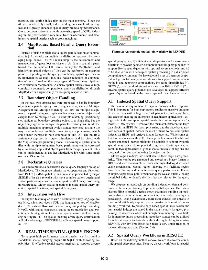
Figure 2: An example spatial join workflow in RESQUE

spatial query types; ii) efficient spatial operators and measurementfunctions to provide geometric computations; iii) query pipelines tosupport diverse spatial queries with optimal access methods; and iv)to be able to run with decoupled spatial processing in a distributedcomputing environment. We have adopted a set of open source spa-tial and geometric computation libraries to support diverse accessmethods and geometric computations, including SpatialIndex [4],GEOS [6], and build additional ones such as Hibert R-Tree [23].Diverse spatial query pipelines are developed to support differenttypes of queries based on the query type and data characteristics.

3.1 Indexed Spatial Query SupportOne essential requirement for spatial queries is fast response.

This is important for both exploratory studies on massive amountsof spatial data with a large space of parameters and algorithms,and decision making in enterprise or healthcare applications. Us-ing spatial index to support spatial queries is a common practice formost SDBMS systems. However, the mismatch between the largedata blocks in HDFS for batch processing and the page based ran-dom access of spatial indexes makes it difficult to pre-store spatialindexes on HDFS and retrieve it later for queries. While some ef-fort has been made on this [39], the approaches are not flexible andthe pre-generated indexes might not be suitable to support dynamicspatial query types. To support indexing based spatial queries, wecombine two approaches: i) global spatial indexes for regions andtiles; and ii) on demand indexing for objects in tiles.

Global region indexes are small due to their large data granu-larity. They can be pre-generated and stored in a binary format inHDFS and shared across cluster nodes through Hadoop distributedcache mechanism. Global region indexing will facilitate regionlevel data filtering and helps improve query performance. For anexample, to process a point or window query we can quickly lookupthe global index to identify the tiles that are relevant for the queryrange.

We propose an approach on building indexes on-demand com-bined with data partitioning to process spatial queries. Our exten-sive profiling of spatial queries shows that index building on mod-ern hardware is not a major bottleneck in large scale spatial queryprocessing. Using dynamically built local indexes for objects intiles could efficiently support spatial queries with minimal indexbuilding overhead. To provide page based spatial index search, thebuilt spatial indexes are stored in the main memory for query pro-cessing. In rare cases where not enough main memory is availablefor in memory index processing, secondary storage can be utilizedfor index storage. Our tests show the indexing building time usingRESQUE with R*-Tree based join takes a very small fraction ofthe overall response time (Section 7.4).

3.2 Spatial Query Workflows in RESQUEBased on the indexing methods above, we are able to create mul-

tiple spatial query pipelines. Next we discuss workflows for spatial

1012

join, spatial containment in detail, and nearest neighbor queries isdiscussed in our previous work [12] which will be skipped here.Spatial Join Workflow. Next we show a workflow of a spatial join(Figure 2), where two datasets from a tile T are joined to find in-tersecting polygon objects. The SQL expression of this query isdiscussed in Section 4.2. Bulk spatial index building is performedon each dataset to generate index files – here we use R*-Trees [14].Hilbert R-Tree can also be used when the objects are in regularshapes and relatively homogenous distribution. The R*-Tree filesare stored in the main memory and contain MBRs in their interiornodes and polygons in their leaf nodes, and will be used for fur-ther query processing. The spatial filtering component performsMBR based spatial join filtering with the two R*-Trees, and re-finement on the spatial join condition is further performed on thepolygon pairs through geometric computations. Much like pred-icate pushdown in traditional database query optimization, spatialmeasurement step is also performed on intersected polygon pairs tocalculate results required, such as overlap area ratio for each pair ofintersecting markups. Other spatial join operators such as overlapsand touches can also be processed similarly.Index Optimization. As data and indexes are read-only and nofurther update is needed, bulk-loading techniques [15] are used. Tominimize the number of pages, the page utilization ratio is alsoset to 100%. In addition, we provide compression to reduce leafnode shape sizes through compact chain code based representation:instead of representing the full coordinates for each x,y coordinate,we use offset from neighboring point to represent the coordinates.The simple chain code compression approach can save 40% spacefor the pathology imaging use case.Spatial Refinement and Measurement. For each pair of markuppolygons whose MBRs intersect, precise geometry computation al-gorithm is used to check whether the two markup polygons actu-ally intersect. Spatial refinement based on geometric computationoften dominates the query execution cost in data-intensive spatialqueries, and could be accelerated through GPU based approach[36]. We are planning to integrate GPU based spatial functionsinto MapReduce in our future work.Spatial Containment Workflow. Spatial containment queries havea slightly different workflow. The spatial containment query rangemay span only a single tile or multiple tiles. Thus, an initial stepwill be to identify the list of intersecting tiles by looking up theglobal tile index, which could filter a large number of tiles. Thetiles whose MBRs intersect with the query range will then be fur-ther processed, where only a single index is used in the spatial fil-tering phase. For an extreme case where the containing shape issmall and lies within a tile, only a single tile is identified for creat-ing the index. For a point query – given a point, find the containingobjects, only a single tile is needed and it has similar workflow asthe small containment query.

4. MAPREDUCE BASED SPATIAL QUERYPROCESSING

RESQUE provides a core query engine to support spatial queries,which enables us to develop high performance large scale spatialquery processing based on MapReduce framework. Our approachis based on spatial data partitioning, tile based spatial query pro-cessing with MapReduce, and result normalization for tile bound-ary objects.

4.1 Spatial Data Partitioning and StorageSpatial data partitioning serves two major purposes. First, it pro-

vides two-dimensional data partitioning and generates a set of tiles,

which become a processing unit for querying tasks. A large set ofsuch tasks can be processed in parallel without data dependance orcommunication requirement. Therefore, spatial partitioning pro-vides not only data partitioning but also computational paralleliza-tion. Last, spatial data partitioning could be critical to mitigate spa-tial data skew. Data skew is a common issue in spatial applications.For example, with a fixed grid partitioning of images into tiles withsize of 4Kx4K, the largest count of objects in a tile is over 20K ob-jects, compared to the average count of 4,291. For OpenStreetMapdataset, by partitioning the space into 1000x1000 fixed grids, theaverage count of objects per tile is 993, but the largest count ofobjects in a tile is 794,429. If there is a parallel spatial query pro-cessing based on tiles, such large skewed tile could significantlyincrease the response time due to the straggling tiles.

As MapReduce provides its own job scheduling for balancingtasks, for spatial data partitioning, we mainly focus on breakinghigh density regions into small ones, and take a recursive partition-ing approach. We either assume the input is a pre-partitioned tilesetwith fixed grid size, which is commonly used for imaging analysisapplications, or pre-generate fixed grid based tileset if no partition-ing exists. We count the number of objects in each tile, and sortthem based on the counts. We define a threshold Cmax as the max-imal count of objects allowed in a tile. We pick all tiles with objectcounts larger than Cmax, and split each of them into two equalhalf-sized tiles based on an optimal direction: x or y. A direction isconsidered optimal if the split along that direction generates a newtile with object count below the threshold, or the two new tiles aremore balanced. This process is repeated until all tiles have countsbelow than Cmax.

After partitioning, each object in a tile is assigned a correspond-ing tile UID. The MBRs of tiles are maintained in a global spatialindex. Note that in the same spatial universe, there could be mul-tiple types of objects with different granularity, e.g., cells versusblood vessels, each dataset of a different type will have its ownseparate partitioning. If there are multiple datasets of the sametype in the same space, e.g., two segmentation results of differentalgorithms, partitioning is considered together for all these datasetsbased on combined object counts.

For data staging into HDFS, we merge all tiles into large filesinstead of storing each tile as a separate file, as the file size fromeach tile could be small, e.g., a few MBs, which are not suitable tobe stored directly into HDFS. This is due to the nature of HDFS,which is optimized for large data blocks (default block size 64MB)for batch processing. Large number of small files leads to deterio-rated performance for MapReduce due to following reasons. First,each file block consumes certain amount of main memory on thecluster namenode and this directly compromises cluster scalabilityand disaster recoverability. Second, in the Map phase, the largenumber of blocks for small files leads to “large number of smallmap tasks” which has significant task-startup overhead.

For objects across tile boundaries, we take the multiple assign-ment approach, where an object intersects with the tile boundarywill be assigned multiple times to all the intersecting tiles [25].Consequently, such boundary objects may participate in multiplequery tasks which could lead to incorrect query results. Therefore,the query results are normalized through an additional boundaryhandling process in which results are rectified (Section 5). Whilethis method will incur redundancy on object storage, the ratio ofboundary objects is usually small (within a few percent in our usecases).

4.2 Spatial Join with MapReduceAs spatial join is among the most commonly used and costly

1013

queries, next we discuss how to map spatial join queries into MapRe-duce computing model. We first show an example spatial joinquery for spatial cross-matching in SQL, as shown in Figure 3.This query finds all intersecting polygon pairs between two resultsets generated from an image by two different methods, and com-pute the overlap ratios (intersection-to-union ratios) and centroiddistances of the pairs. The table markup polygon represents theboundary as polygon, algorithm UID as algrithm uid. The SQLsyntax comes with spatial extensions such as spatial relationshipoperator ST INTERSECTS, spatial object operators ST INTERSECTIONand ST UNION, and spatial measurement functions ST CENTROID,ST DISTANCE, and ST AREA.

1: SELECT2: ST_AREA(ST_INTERSECTION(ta.polygon,tb.polygon))/3: ST_AREA(ST_UNION(ta.polygon,tb.polygon)) AS ratio,4: ST_DISTANCE(ST_CENTROID(tb.polygon),5: ST_CENTROID(ta.polygon)) AS distance,6: FROM markup_polygon ta JOIN markup_polygon tb ON8: ST_INTERSECTS(ta.polygon, tb.polygon) = TRUE9: WHERE ta.algrithm_uid=’A1’ AND tb.algrithm_uid=’A2’ ;

Figure 3: An example spatial join (cross-matching) query

For simplicity, we first present how to process the spatial joinabove with MapReduce, by ignoring boundary objects, and thenwe come back to the boundary handling in Section 5. A MapRe-duce program for spatial join query (Figure 3) will have similarstructure as a regular relational join operation, but with all the spa-tial part executed by invoking RESQUE engine within the program.According to the equal-join condition, the program uses the Stan-dard Repartition Algorithm [16] to execute the query. Based onthe MapReduce structure, the program has three main steps: i) Inthe map phase, the input table is scanned, and the WHERE con-dition is evaluated on each record. Only those records that satisfythe WHERE condition are emitted with tile uid is as key. ii) In theshuffle phase, all records with the same tile uid would be sortedand prepared for the reducer operation. iii) In the reduce phase, thetile based spatial join operation is performed on the input recordsand the spatial operations are executed by invoking the RESQUEengine (Section 3).

The workflow of the map function is shown in the map functionin Algorithm 2. Each record in the table is converted into the mapfunction input key/value pair (k, v), where k is the byte offset ofthe line in the file, and v is the record. Inside the map function,if the record can satisfy the select condition, then an intermediatekey/value pair is generated. The intermediate key is the tile uidof this record, and the intermediate value is the combination ofcolumns which are specified in the select clause. Note that the in-termediate key/values will participate in a two-table join, and a tagmust be attached to the value in order to indicate which table therecord belongs to. Besides, since the query for this case is a self-join, we use a shared scan in the map function to execute the datafilter operations on both instances of the same table. Therefore, asingle map input key/value could generate 0, 1 or 2 intermediatekey/value pairs, according to the SELECT clause and the values ofthe record.

The shuffle phase is performed by Hadoop internally, which groupsdata by tile UIDs. The workflow of the reduce function is shown inthe reduce function in Algorithm 2. According to the main structureof the program, the input key of the reduce function is the join key(tile uid), and the input values of the reduce function are all recordswith the same tile uid. In the reduce function, we first initialize twotemporary files, then we dispatch records into corresponding files.After that, we invoke RESQUE engine to build R*-tree indexes

Algorithm 2: MapReduce program for spatial join query

function Map(k,v):tile uid = projectKey(v);join seq = projectJoinSequence(v);record = projectRecord(v);v = concat(join seq,record);emit( tile uid , v);

function JoinReduce(k,v):/* arraylist holds join objects */join set = [ ] ;for vi in v do

join seq = projectJoinSequence(vi);record = projectRecord(vi);if join seq == 0 then

join set[0].append(record);if join seq == 1 then

join set[1].append(record);

/* library call to RESQUE */plan = RESQUE.genLocalPlan(join set);result = RESQUE.processQuery(plan);for item in result do

emit(item);

and execute the query. The execution result data sets are stored ina temporary in-memory file. Finally we parse that file, and outputthe result to HDFS. Note that the function RESQUE.processQueryhere performs multiple spatial opeartions together, including eval-uation of WHERE condition, projection, and computation (e.g.,ST intersection and ST area), which could be customized.

4.3 Other Spatial Query TypesOther spatial queries can follow a similar process pattern as shown

in Algorithm 1. Spatial selection/containment is a simple querytype in which objects geometrically contained in selection regionare returned. For example, in a medical imaging scenario, usersmay be interested in the cell features which are contained in a can-cerous tissue region. Thus, a user can issue a simple query as shownin Figure 4 to retrieve cancerous cells.

1: SELECT * FROM markup_polygon m, human_markup h2: WHERE h.name=’cancer’ AND3: ST_CONTAINS(h.region, m.polygon) = TRUE;

Figure 4: An Example Containment Query in SQL

Since data is partitioned into tiles, containment queries can beprocessed in a filter-and-refine fashion. In the filter step, tiles whichare disjoined from the query region can be filtered. In the refine-ment step, the candidate objects are checked with precise geometrytest. The global region index is used to generate a selective tablescan operation which only scans the file splits which potentiallycontain the query results. The query would be translated into amap only MapReduce program shown in Algorithm 3. Supportof multi-way spatial join queries and nearest neighbor queries fol-low a similar pattern and are discussed in our previous work [12].Figure 4 illustrates a containment query in which the task is to re-trieve all the cells which are spatially contained in a region whichis marked as cancereous.

5. BOUNDARY HANDLING

1014

Algorithm 3: MapReduce program for containment query

function Map(k,v):/* a arraylist holds spatial objects */candidate set = [ ] ;tile id = projectKey(v);

for vi in v dorecord = projectRecord(vi);candidate set.append(record);

tile boundary =getTileBoundary( tile id);if queryRegion.contains(tile boundary) then

emitAll(candidate set);else

if queryRegion.intersects(tile boundary) thenfor record in candidate set do

if queryRegion.contains(record) thenemit(record);

Tile is the basic parallelization unit in Hadoop-GIS. However, intile based partitioning, some spatial objects may lie on tile bound-aries. We define such an object as boundary object of which spa-tial extent crosses multiple tile boundaries. For example, in Fig-ure 5 (left), the object p is a boundary object which crosses the tileboundaries of tiles S and T. In general, the fraction of boundaryobjects is inversely proportional to the size of the tile. As tile sizegets smaller, the percentage of boundary objects increases.

There are two basic approaches to handle boundary objects. Theyeither have to be specially processed to guarantee query semanticsand correctness, or they can be simply discarded. The latter is suit-able for a scenario where approximate query results are needed, andquery results would not be effected by the tiny fraction of bound-ary objects. Whereas in many other cases, accurate and consistentquery results are required and the boundary objects need to be han-dled properly.

S T Sps

Tpt

qqp

+

Figure 5: Boundary object illustration

Hadoop-GIS remedies the boundary problem in a simple buteffective way. If a query requires to return complete query re-sult, Hadoop-GIS generates a query plan which contains a pre-processing task and a post-processing task. In the pre-processingtask, the boundary objects are duplicated and assigned to multi-ple intersecting tiles (multiple assignment). When each tile is pro-cessed independently during query execution, the results are not yetcorrect due to the duplicates. In the post-processing step, resultsfrom multiple tiles will be normalized, e.g., to eliminate duplicaterecords by checking the object uids, which are assigned internallyand globally unique. For example, when processing the spatial joinquery, the object p is duplicated to tiles S and T as ps and pt (Fig-ure 5 right). Then the same process of join processing follows as ifthere are no boundary objects. In the post-processing step, objectswill go through a filtering process in which duplicate records areeliminated.

Algorithm 4: Boundary aware spatial join processing

function Map(k,v):tile id = projectKey(v);record = projectRecord(v);if isBoundaryObject(record, tile id) then

tiles = getCrossingTiles(record) ;/* replicate to multiple tiles */for tile id in tiles do

emit(tile id , v);

function JoinReduce(k,v):/* performs tile based spatial join,

same as reduce function inAlgorithm 2 */

function Map(k,v):uid1 = projectUID(v,1);uid2 = projectUID(v,2);key = concat(uid1,uid2);emit(key,v);

/* Hadoop sorts records by key andshuffles them */

function Reduce(k,v):for records in v do

if isUniq(record) thenemit(record);

Intuitively, such approach would incur extra query processingcost due to the replication and duplicate elimination steps. How-ever, this extra cost is very small compared to the overall queryprocessing time, and we will experimentally quantify such over-head later in Section 7.

6. INTEGRATION WITH HIVEHive [32] is an open source MapReduce based query system that

provides a declarative query language for users. By providing avirtual table like view of data, SQL like query language HiveQL,and automatic query translation, Hive achieves scalability while itgreatly simplifies the effort on developing applications in MapRe-duce. HiveQL supports a subset of standard ANSI SQL statementswhich most data analysts and scientists are familiar with.

6.1 ArchitectureTo provide an integrated query language and unified system on

MapReduce, we extend Hive with spatial query support by extend-ing HiveQL with spatial constructs, spatial query translation andexecution, with integration of the spatial query engine into Hivequery engine (Figure 1). We call the language QLSP , and the Hiveintegrated version of Hadoop-GIS as HiveSP . An example spatialSQL query is shown in Figure 3. The spatial indexing aware queryoptimization will take advantage of RESQUE for efficient spatialquery support in Hive.

There are several core components in HiveSP to provide spatialquery processing capabilities. i) Spatial Query Translator parsesand translates SQL queries into an abstract syntax tree. We extendthe HiveQL translator to support a set of spatial query operators,spatial functions, and spatial data types. ii) Spatial Query Opti-mizer takes an operator tree as an input and applies rule based op-timizations such as predicate push down or index-only query pro-

1015

cessing. iii) Spatial Query Engine supports following infrastruc-ture operations: spatial relationship comparison, such as intersects,touches, overlaps, contains, within, disjoint, spatial measurements,such as intersection, union, distance, centroid, area; and spatialaccess methods for efficient query processing, such as R∗-Tree,Hilbert R-Tree and Voronoi Diagram. The engine is compiled asa shared library and can be easily deployed.

Users interact with the system by submitting SQL queries. Thequeries are parsed and translated into an operator tree, and thequery optimizer applies heuristic rules to the operator tree to gen-erate an optimized query plan. For a query with spatial query op-erator, MapReduce codes are generated, which call an appropriatespatial query pipeline supported by the spatial query engine. Gen-erated MapReduce codes are submitted to the execution engine toreturn intermediate results, which can be either returned as finalquery results or be used as input for next query operator. Spatialdata is partitioned based on the attribute defined in the “PARTI-TION BY” clause and staged to the HDFS.

6.2 Query ProcessingHiveSP uses the traditional plan-first, execute-next approach for

query processing, which consists of three steps: query translation,logical plan generation, and physical plan generation. To processa query expressed in SQL, the system first parses the query andgenerates an abstract syntax tree. Preliminary query analysis isperformed in this step to ensure that the query is syntactically andgrammatically correct. Next, the abstract syntax tree is translatedinto a logical plan which is expressed as an operator tree, and sim-ple query optimization techniques such as predicate push down andcolumn pruning are applied in this step. Then, a physical plan isgenerated from the operator tree which eventually consists of se-ries of MapReduce tasks. Finally, the generated MapReduce tasksare submitted to the Hive runtime for execution.

Major differences between Hive and HiveSP are in the logicalplan generation step. If a query does not contain any spatial oper-ations, the resulting logical query plan is exactly the same as theone generated from Hive. However, if the query contains spatialoperations, the logical plan is regenerated with special handling ofspatial operators. Specifically, two additional steps are performedto rewrite the query. First, operators involving spatial operationsare replaced with internal spatial query engine operators for tilelevel query processing. Second, serialization/deserialization oper-ations are added before and after the spatial operators to prepareHive for communicating with the spatial query engine.

An example query plan is given in Figure 6, which is generatedfrom translating SQL query in Figure 3. Notice that the spatialjoin operator is implemented as reduce side join and the spatialdata table is partitioned by tiles for parallel processing, with a userspecified partition column during virtual table definition.

6.3 SoftwareHadoop-GIS has two forms: the standalone library version which

can be invoked through customizations, and Hive integrated versionHiveSP . HiveSP is designed to be completely hot-swappable withHive. Hive users only need to deploy the spatial query engine onthe cluster nodes, and turn the spatial query processing switch on.Any query that runs on Hive can run on HiveSP without modifica-tion.

The spatial query engine is written in C++ and compiled as ashared library. We use libspatial library [4] for building R*-Tree index, and the library is extended to support index based spa-tial operations such as two-way, multi-way spatial joins and nearestneighbor search [12].

Map

Reduce

TableScanOperator

table: ta

TableScanOperator

table: tb

FilterOperator

predicate: provenance=’A1’

FilterOperator

predicate: provenance=’A2’

ReduceSinkOperator

partition col: tile id

ReduceSinkOperator

partition col: tile id

SpatialJoinOperator

predicate:

ST Intersects(col[0.0],col[0.1])

SelectOperator

expressions: col[0],col[2] ...

FileOutputOperator

table: temp tb

Figure 6: Two-way spatial join query plan

To use the system, users follow the same user guidelines of us-ing Hive. First of all, users need to create all the necessary tableschema which will be persisted to the metastore as metadata. Spa-tial columns need to be specified with corresponding data typesdefined in ISO SQL/MM Spatial. Spatial partitioning column canalso be specified. After the schema creation, users can load thedata through Hive data loading tool. Once data is loaded, users canbegin to write spatial SQL queries.

7. PERFORMANCE STUDYWe study the performance of RESQUE query engine versus other

SDBMS engines, the performance of Hadoop-GIS versus parallelSDBMS, scalability of Hadoop-GIS in terms of number of reducersand data size, and query performance with boundary handling.

7.1 Experimental SetupHadoop-GIS: We use a cluster with 8 nodes and 192 cores. Each ofthese 8 nodes comes with 24 cores (AMD 6172 at 2.1GHz), 2.7TBhard drive at 7200rpm and 128GB memory. A 1Gb interconnect-ing network is used for node communication. The OS is CentOS5.6 (64 bit). We use the Cloudera Hadoop 2.0.0-cdh4.0.0 as ourMapReduce platform, and Apache Hive 0.7.1 for HiveSP . Most ofthe configuration parameters are set to their default value, exceptthe JVM maximum heap size which is set to 1024MB. The systemis configured to run a maximum of 24 map or reduce instances oneach node. Datasets are uploaded to the HDFS and the replicationfactor is set to 3 on each datanode.DBMS-X: To have a comparison between Hadoop-GIS and par-allel SDBMS, we installed a commercial DBMS (DBMS-X) withspatial extensions and partitioning capabilities on two nodes. Eachnode comes with 32 cores, 128GB memory, and 8TB RAID-5 drivesat 7200rpm. The OS for the nodes is CentOS 5.6 (64 bit). Thereare a total of 30 database partitions, 15 logical partitions on eachnode. With the technical support from the DBMS-X vendor, theparallel SDBMS has been tuned with many optimizations, suchas co-location of common joined datasets, replicated spatial refer-ence tables, proper spatial indexing, and query hints. For RESQUEquery engine comparison, we also install PostGIS (V1.5.2, singlepartition) on a cluster node.

7.2 Dataset DescriptionWe use two real world datasets: pathology imaging, and Open-

StreetMap.

1016

Pathology Imaging (PI). This dataset comes from image analysisof pathology images, by segmenting boundaries of micro-anatomicobjects such as nuclei and tumor regions. The images are pro-vided by Emory University Hospital. Spatial boundaries have beenvalidated, normalized, and represented in WKT format. We havedataset sizes at 1X (18 images, 44GB), 3X (54 images, 132GB),5X (90 images, 220GB), 10X (180 images, 440GB), and 30X (540images, 1,320GB) for different testings. The average number ofnuclei per image is 0.5 million, and 74 features are derived for eachnucleus.OpenStreetMap (OSM). OSM [8] is a large scale map projectthrough extensive collaborative contribution from a large numberof community users. It contains spatial representation of geometricfeatures such as lakes, forests, buildings and roads. Spatial objectsare represented by a specific type such as points, lines and poly-gons. We download the dataset from the official website, and parseit into a spatial database. The table schema is simple and it hasroughly 70 columns. We use the polygonal representation tablewith more than 87 million records. To be able to run our queries,we construct two versions of the OSM dataset, one from a latestversion, and another smaller one from an earlier version released in2010. The dataset is also dumped as text format for Hadoop-GIS.

7.3 Query BenchmarkingWe use three typical queries for the benchmark: spatial join (spa-

tial cross-matching), spatial selection (containment query), and ag-gregation. Many other complex queries can be decomposed intothese queries, for example, a spatial aggregation can be run in twosteps: first step for spatial object filtering with a containment query,followed by an aggregation on filtered spatial objects. The spatialjoin query on PI dataset is demonstrated in Figure 3 for joining twodatasets with an intersects predicate. Another similar spatial joinquery on OSM dataset is also constructed to find changes in spa-tial objects between two snapshots. We construct a spatial contain-ment query, illustrated in Figure 4 for PI case, to retrieve all objectswithin a region, where the containment region covers a large areain the space. A similar containment query is also constructed forOSM dataset with a large query region. For aggregation query, wecompute the average area and perimeter of polygons of differentcategories, with 100 distinct labels.

7.4 Performance of RESQUE EngineStandalone Performance. An efficient query engine is a criticalbuilding block for a large scale system. To test the standaloneperformance of RESQUE, we run it on a single node as a singlethread application. The spatial join query is used as a represen-tative benchmark. We first test the effect of spatial indexing, bytaking a single tile with two result sets (5506 markups vs 5609markups), and the results are shown in Figure 8(a). A brute-forceapproach compares all possible pairs of boundaries in a nested loopmanner without using any index, and takes 673 minutes. Such slowperformance is due to polynomial complexity on pair-wise com-parisons and high complexity on geometric intersection testing.An optimized brute-force approach will first eliminate all the non-intersecting markup pairs by using a MBR based filtering. Thenit applies the geometry intersection testing algorithm on the candi-date markup pairs. This approach takes 4 minutes 41 seconds, a bigsaving with minimized geometric computations. Using RESQUEwith indexing based spatial join, the number of computations is sig-nificantly reduced, and it only takes 10 seconds. When profiling thecost for RESQUE, we observe that reading and parsing cost is 30%,R*-Tree construction cost is 0.2%, MBR filtering cost is 0.67%,and spatial refinement and measurement cost is 69.13%. With fast

development of CPU speed, spatial index construction takes verylittle time during the query process, which motivates us to developan index-on-demand approach to support spatial queries. We canalso see that geometric computation dominates the cost, which canbe accelerated through parallel computation on a cluster.

10

100

1000

10000

SDBMS X

PostGISRESQUE (w/ indexing cost)

Brute Force w/ MBR

Seco

nds

Brute Force

(a) Single tile

RESQUE PostGIS SDBMS X0

500

1000

1500

2000

Secon

ds

Loading Indexing Querying

(b) Single image

Figure 8: Performance of RESQUE

Data Loading Efficiency. Another advantage of RESQUE is itslight data loading cost compared to SDBMS approach. We runthree steps to get the overall response time (data loading, indexingand querying) on three systems: RESQUE on a single slot MapRe-duce with HDFS, PostGIS and SDBMS-X with a single partition.The data used for the testing are two results from a single image(106 tiles, 528,058 and 551,920 markups respectively). As shownin Figure 8(b), data loading time for REQUE is minimal comparedto others. With controlled optimization, RESQUE outperforms onthe overall efficiency.

7.5 Performance of Hadoop­GIS

7.5.1 Hadoop­GIS versus Parallel SDBMSFor the purpose of comparison, we run the benchmark queries on

both Hadoop-GIS and DBMS-X on the PI dataset. The data is par-titioned based on tile UIDs – boundary objects are ignored in thetesting as handling boundary objects in SDBMS is not supporteddirectly. Figure 7 shows the performance results. The horizon-tal axis represents the number of parallel processing units (PPU),and the vertical axis represents query execution time. For the par-allel SDBMS, the number of PPUs corresponds to the number ofdatabase partitions. For Hadoop-GIS, the number of PPU corre-sponds to the number of mapper and reducer tasks.Join Query. As the figure 7(a) shows, both systems exhibit goodscalability, but overall Hadoop-GIS performs much better com-pared to DBMS-X, which has already been well tuned by the ven-dor. Across different numbers of PPUs, Hadoop-GIS is more thana factor of two faster than DBMS-X. Given that DBMS can in-telligently place the data in storage and can reduce IO overheadby using index based record fetching, it is expected to have betterperformance on IO heavy tasks. However, a spatial join involvesexpensive geometric computation, and the query plan generated bythe DBMS is suboptimal for such tasks. Another reason for theperformance of DBMS-X is because of its limited capability onhandling computational skew, even though the built-in partitioningfunction generates a reasonably balanced data distribution. Hadoophas an on-demand task scheduling mechanism which can help alle-viate such computational skew.Containment Query. For containment queries, Hadoop-GIS out-performs DBMS-X on a smaller scale and has a relatively flat per-formance across different number of PPUs. However, DBMS-Xexhibits better scalability when scaled out with larger number ofpartitions. Recall that, in Hadoop-GIS, a containment query is im-plemented as a Map only MapReduce job, and the query itself is

1017

5 10 20 300

500

1000

1500

2000

2500

Tim

e (s

econ

ds)

Processing Units

Hadoop-GIS DBMS-X

(a) Join

5 10 20 300

10

20

30

40

50

60

70

Tim

e (s

econ

ds)

Processing Units

Hadoop-GIS DBMS-X

(b) Containment

5 10 20 300

20

40

60

80

100

120

Tim

e (s

econ

ds)

Processing Units

Hadoop-GIS DBMS-X

(c) Aggregation

Figure 7: Performance Comparison between Hadoop-GIS and DBMS-X on PI Dataset

less computationally intensive compared to the join query. There-fore, the time is actually being spent on reading in a file split, pars-ing the objects, and checking if the object is contained in the queryregion. On the other hand, DBMS-X can take advantage of a spa-tial index and can quickly filter out irrelevant records. Therefore itis not surprising that DBMS-X has slightly better performance forcontainment queries.Aggregation Query. Figure 7(c) demonstrates that DBMS-X per-forms better than Hadoop-GIS on aggregation task. One reasonfor this is that Hadoop-GIS has the record parsing overhead. Bothsystems have similar query plans - a whole table scan followed byan aggregation operation on the spatial column, which have sim-ilar I/O overhead. In Hadoop-GIS, however, the records need tobe parsed in real-time, whereas in DBMS-X records are pre-parsedand stored in binary format.

In a summary, Hadoop-GIS performs better in compute-intensiveanalytical tasks and exhibits nice scalability - a highly desirablefeature for data warehousing applications. Moreover, it needs muchless tuning effort compared to the database approach. However,MapReduce based approach may not be the best choice if the querytask is small, e.g., queries to retrieve a small number of objects.

7.5.2 Performance on OpenStreetMap Dataset

0 20 40 60 80 100 120 140 160 180 200400

600

800

1000

1200

1400

1600

1800

2000

2200

2400

Processing Unit

Tim

e (s

econ

ds)

(a) OSM join

5 10 20 30 40 50 1000

100

200

300

400

500

600

Tim

e (s

econ

ds)

Processing Unit

(b) OSM containment

Figure 9: Performance of Hadoop-GIS on OSMWe have also tested performance and scalability of Hadoop-GIS

on OSM dataset, which contains geospatial objects. To test sys-tem scalability, we run the same types of queries as on the PIdataset. For the join query, the query returns objects which havebeen changed in the newer version of the dataset. Therefore, thejoin predicate becomes ST EQUAL = FALSE.

Figure 9 shows the performance results for Hadoop-GIS on OSMdataset. As Figure 9(a) shows, Hadoop-GIS exhibits very nice scal-ability on the join task. When the number of available processingunits is increased to 40 from 20, the query time nearly reduced intohalf, which is almost a linear speed-up. With increase of the num-ber of PPUs, there is a continuous drop on the query time.

Figure 9(b) illustrates the containment query performance onOSM dataset, where running time is less than 100 seconds. The

variance of query performance across different number of PPUs isflat, due to the fact that containment queries are relatively IO inten-sive.

7.5.3 Scalability of Hadoop­GISFigure 10(a) shows the scalability of the system. Datasets used

include: 1X, 3X, 5X, and 10X datasets, with varying number ofPPUs. We can see a continuous decline of query time when thenumber of reducers increases. It achieves a nearly linear speed-up, e.g., time is reduced to by half when the number of reducersis increased from 20 to 40. The average querying time per imageis about 9 seconds for the 1X dataset with all cores, comparingwith 22 minutes 12 seconds in a single partition PostGIS. The sys-tem has a very good scale up feature. As the figure shows, queryprocessing time increases linearly with dataset size. The time forprocessing the join query on 10X dataset is roughly 10 times of thetime for processing a 1X dataset.

7.6 Boundary Handling OverheadWe run the join query on PI dataset to measure the overhead in

boundary handling step. Figure 10(b) shows the performance ofspatial join query with boundary handling. The blue bars repre-sent the cost of processing the query, and the green bars representthe cost of amending the results. As the figure shows, the cost ofboundary handling is very small. Boundary handling overhead de-pends on two factors – the number of boundary objects and the sizeof the query output. If the number of objects on the tile boundaryaccounts for a considerable fraction of the dataset, the overheadshould not dominate the query processing time. Therefore, we testthe join query on the same dataset in which the number of bound-ary objects is deliberately increased. Figure 10(c) shows the spatialjoin query performance with different fraction of boundary objects.The lines represent query performance with varying percentage ofboundary objects as shown in the legend. It is clear from the figurethat, the boundary handling overheard increases linearly with thepercentage of boundary objects.

In Figure 10(c), we show the performance when the percentageof boundary objects is as high as 11.7%. In reality, the number ofobjects is much less than this number. We have performed an ex-periment with the OSM dataset in which the dataset is partitionedinto 1 million tiles. Even in such a fine granular level of partition-ing, the number of objects lying on the grid boundary is less than2%.

8. RELATED WORKParallel SDBMS has been used for managing and querying large

scale spatial data based on shared nothing architecture [28], suchas Greenplum, IBM Netezza, Teradata, and partitioned version of

1018

0 20 40 60 80 100 120 140 160 180 2000

1000

2000

3000

4000

5000

Tim

e (s

econ

ds)

Processing Unit

1X (18 images) 3X (54 images) 5X (90 images) 10X (180 images)

(a) Scalability Test

10 20 40 60 80 100 1400

50

100

150

200

250

300

350

400

450

500

550

Tim

e (s

econ

ds)

Processing Unit

merge cost join cost

(b) Boundary handling overhead

0 20 40 60 80 1000

100

200

300

400

500

600

700

Tim

e (s

econ

ds)

Parallel Unit

2.6 % 6.5 % 11.7 %

(c) Overhead variation

Figure 10: Scalability of Hadoop-GIS & boundary handling overhead

IBM DB2 Spatial Extender, Oracle Spatial, MS SQL Server Spa-tial, and PostGIS. These approaches lack the framework for spatialpartitioning and boundary object handling. Data loading speed isa major bottleneck for SDBMS based solutions [29], especially forcomplex structured spatial data types [35]. We have previously de-veloped a parallel SDBMS based approach PAIS [34, 35, 9] basedon DB2 DPF with reasonable scalability, but the approach is highlyexpensive on software license and hardware requirement[29], andrequires sophisticated tuning and maintenance. The objective of thework presented in this paper is to provide a scalable and cost effec-tive approach to support expressive and high performance spatialqueries. The Sloan Digital Sky Survey project (SDSS) [3] cre-ates a high resolution multi-wavelength map of the Northern Skywith 2.5 trillion pixels of imaging, and takes a large scale paralleldatabase approach. SDSS provides a high precision GIS system forastronomy, implemented as a set of UDFs. The database runs onGrayWulf architecture [31] through collaboration with Microsoft.

Partitioning based approach for parallelizing spatial joins is dis-cussed in [40], which uses the multiple assignment, single join ap-proach with partitioning-based spatial join algorithm. The authorsalso provide re-balancing of tasks to achieve better parallelization.We take the same multiple assignment approach for partitioning,but use index based spatial join algorithm, and rely on MapReducefor load balancing. R-Tree based parallel spatial join is also pro-posed in early work [17] with a combined shared virtual memoryand shared nothing architecture. Recently we have exploited mas-sive data parallelism by developing GPU aware parallel geometriccomputation algorithms to support spatial joins running on desktopmachines [36]. Integrating GPU into our MapReduce pipeline isamong our future work.

Spatial support has been extended to NoSQL based solutions,such as neo4j/spatial [2] and GeoCouch [1]. These approachesbuild spatial data structures and access methods on top of key-valuestores, thus take advantage of the scalability. However, these ap-proaches support limited queries, for example, GeoCouch supportsonly bounding box queries, and there is no support of the analyticalspatial queries for spatial data warehousing applications.

In [18], an approach is proposed on bulk-construction of R-Treesthrough MapReduce. In [38], a spatial join method on MapReduceis proposed for skewed spatial data, using an in-memory basedstrip plane sweeping algorithm. It uses a duplication avoidancetechnique which could be difficult to generalize for different querytypes. Hadoop-GIS takes a hybrid approach on combining parti-tioning with indexes and generalizes the approach to support mul-tiple query types. Besides, our approach is not limited to memorysize. VegaGiStore [39] tries to provide a Quadtree based globalpartitioning and indexing, and a spatial object placement structuresthrough Hibert-ordering with local index header and real data. The

global index links to HDFS blocks where the structures are stored.It is not clear how boundary objects are handled in partitioning,and how parallel spatial join algorithm is implemented. Work in[5] takes a fixed grid partitioning based approach and uses sweepline algorithm for processing distributed joins on MapReduce. Itis unclear how the boundary objects are handled, and no perfor-mance study is available at the time of evaluation. The work in[22] presents an approach for multi-way spatial join for rectanglebased objects, with a focus on minimizing communication cost. AMapReduce based Voronoi diagram generation algorithm is pre-sented in [13]. In our work in [12], we present preliminary resultson supporting multi-way spatial join queries and nearest neighborqueries for pathology image based applications. This paper has sig-nificantly generalized the work to provide a generic framework forsupporting multiple types of spatial applications, and a systematicapproach for data partitioning and boundary handling.

Comparisons of MapReduce and parallel databases for struc-tured data are discussed in [29, 20, 30]. Tight integration of DBMSand MapReduce is discussed in [10, 37]. MapReduce systemswith high-level declarative languages include Pig Latin/Pig [27,21], SCOPE [19], and HiveQL/Hive [32]. YSmart provides an op-timized SQL to MapReduce job translation and is recently patchedto Hive. Hadoop-GIS takes an approach that integrates DBMS’sspatial indexing and declarative query language capabilities intoMapReduce.

9. CONCLUSION AND DISCUSSION“Big” spatial data from imaging and spatial applications share

many similar requirements for high performance and scalabilitywith enterprise data, but has its own unique characteristics – spa-tial data are multi-dimensional and spatial query processing comeswith high computational complexity. In this paper, we presentHadoop-GIS, a solution that combines the benefit of scalable andcost-effective data processing with MapReduce, and the benefitof efficient spatial query processing with spatial access methods.Hadoop-GIS achieves the goal through spatial partitioning, parti-tion based parallel processing over MapReduce, effective handlingof boundary objects to generate correct query results, and multi-level spatial indexing supported customizable spatial query engine.Our experiment results on two real world use cases demonstratethat Hadoop-GIS provides a scalable and effective solution for an-alytical spatial queries over large scale spatial datasets.

Our work was initially motivated by the use case of pathologyimaging. We started from a parallel SDBMS based solution [35]and experienced major problems such as the data loading bottle-neck, limited support of complex spatial queries, and the high costof software and hardware. Through the development and deploy-

1019

ment of MapReduce based query processing, we are able to providescalable query support with cost-effective architecture [12]. In thispaper, we have generalized the approach to provide a solution thatcan be used to support various spatial applications.

Ongoing work includes support of 3D pathology analytical imag-ing. 3D examinations of tissues at microscopic resolution are nowpossible and have significant potential to enhance the study of bothnormal and disease processes, by exploring structural changes orspatial relationship of disease features. A single 3D image consistsof around a thousand slices and consumes more than 1TB storage,and spatial queries on massive 3D geometries pose many new chal-lenges. Another ongoing work is to support queries for global spa-tial patterns such as density and directional patterns. We are alsoworking on integrating GPU based spatial operations [36] into thequery pipeline.

10. ACKNOWLEDGMENTSThis work is supported in part by PHS Grant UL1RR025008

from the CTSA program, R24HL085343 from the NHLBI, by GrantNumber R01LM009239 from the NLM, by NCI Contract No. N01-CO-12400 and 94995NBS23 and HHSN261200800001E, by NSFCNS 0615155, CNS-1162165, 79077CBS10, CNS-0403342, OCI-1147522, and P20 EB000591 by the BISTI program. IBM providesacademic license for DB2. David Adler and Susan Malaika fromIBM provided many insightful suggestions.

11. REFERENCES[1] Geocouch. https://github.com/couchbase/geocouch/.[2] neo4j/spatial. https://github.com/neo4j/spatial.[3] The sloan digital sky survey project (sdss). http://www.sdss.org.[4] Spatial index library. http://libspatialindex.github.com.[5] Spatialhadoop. http://spatialhadoop.cs.umn.edu/.[6] Geos. http://trac.osgeo.org/geos, 2013.[7] Hadoop-GIS wiki. https://web.cci.emory.edu/confluence

/display/hadoopgis, 2013.[8] Openstreetmap. http://www.openstreetmap.org, 2013.[9] Pathology analytical imaging standards.

https://web.cci.emory.edu/confluence /display/PAIS, 2013.[10] A. Abouzeid, K. Bajda-Pawlikowski, D. Abadi, A. Silberschatz, and

A. Rasin. Hadoopdb: an architectural hybrid of mapreduce and dbmstechnologies for analytical workloads. Proc. VLDB Endow.,2:922–933, August 2009.

[11] A. Aji. High performance spatial query processing for large scalescientific data. In Proceedings of the on SIGMOD/PODS 2012 PhDSymposium, pages 9–14, New York, NY, USA, 2012. ACM.

[12] A. Aji, F. Wang, and J. H. Saltz. Towards building a highperformance spatial query system for large scale medical imagingdata. In SIGSPATIAL/GIS, pages 309–318, 2012.

[13] A. Akdogan, U. Demiryurek, F. Banaei-Kashani, and C. Shahabi.Voronoi-based geospatial query processing with mapreduce. InCLOUDCOM, pages 9–16, 2010.

[14] N. Beckmann, H. Kriegel, R. Schneider, and B. Seeger. The r*-tree:An efficient and robust access method for points and rectangles. InSIGMOD, 1990.

[15] J. V. d. Bercken and B. Seeger. An evaluation of generic bulk loadingtechniques. In VLDB, pages 461–470, 2001.

[16] S. Blanas, J. M. Patel, V. Ercegovac, J. Rao, E. J. Shekita, andY. Tian. A comparison of join algorithms for log processing inmapreduce. In SIGMOD, 2010.

[17] T. Brinkhoff, H.-P. Kriegel, and B. Seeger. Parallel processing ofspatial joins using r-trees. In ICDE, 1996.

[18] A. Cary, Z. Sun, V. Hristidis, and N. Rishe. Experiences onprocessing spatial data with mapreduce. In SSDBM, pages 302–319,2009.

[19] R. Chaiken, B. Jenkins, P. Larson, B. Ramsey, D. Shakib, S. Weaver,and J. Zhou. SCOPE: easy and efficient parallel processing ofmassive data sets. PVLDB, 1(2):1265–1276, 2008.

[20] J. Dean and S. Ghemawat. Mapreduce: a flexible data processingtool. Commun. ACM, 53(1):72–77, 2010.

[21] A. Gates, O. Natkovich, S. Chopra, P. Kamath, S. Narayanam,C. Olston, B. Reed, S. Srinivasan, and U. Srivastava. Building a highlevel dataflow system on top of MapReduce: The Pig experience.PVLDB, 2(2):1414–1425, 2009.

[22] H. Gupta, B. Chawda, S. Negi, T. A. Faruquie, L. V. Subramaniam,and M. Mohania. Processing multi-way spatial joins on map-reduce.In EDBT, pages 113–124, 2013.

[23] I. Kamel and C. Faloutsos. Hilbert r-tree: An improved r-tree usingfractals. In VLDB, pages 500–509, 1994.

[24] R. Lee, T. Luo, Y. Huai, F. Wang, Y. He, and X. Zhang. Ysmart: Yetanother sql-to-mapreduce translator. In ICDCS, 2011.

[25] M.-L. Lo and C. V. Ravishankar. Spatial hash-joins. In SIGMOD,pages 247–258, 1996.

[26] M. A. Nieto-Santisteban, A. R. Thakar, and A. S. Szalay.Cross-matching very large datasets. In NSTC NASA Conference,2007.

[27] C. Olston, B. Reed, U. Srivastava, R. Kumar, and A. Tomkins. Piglatin: a not-so-foreign language for data processing. In SIGMOD,2008.

[28] J. Patel, J. Yu, N. Kabra, K. Tufte, B. Nag, J. Burger, N. Hall,K. Ramasamy, R. Lueder, C. Ellmann, J. Kupsch, S. Guo, J. Larson,D. De Witt, and J. Naughton. Building a scaleable geo-spatial dbms:technology, implementation, and evaluation. In SIGMOD, SIGMOD’97, pages 336–347, 1997.

[29] A. Pavlo, E. Paulson, A. Rasin, D. J. Abadi, D. J. DeWitt, S. Madden,and M. Stonebraker. A comparison of approaches to large-scale dataanalysis. In SIGMOD, pages 165–178, 2009.

[30] M. Stonebraker, D. J. Abadi, D. J. DeWitt, S. Madden, E. Paulson,A. Pavlo, and A. Rasin. Mapreduce and parallel dbmss: friends orfoes? Commun. ACM, 53(1):64–71, 2010.

[31] A. S. Szalay, G. Bell, J. vandenBerg, A. Wonders, R. C. Burns,D. Fay, J. Heasley, T. Hey, M. A. Nieto-Santisteban, A. Thakar,C. v. Ingen, and R. Wilton. Graywulf: Scalable clustered architecturefor data intensive computing. In HICSS, pages 1–10, 2009.

[32] A. Thusoo, J. S. Sarma, N. Jain, Z. Shao, P. Chakka, S. Anthony,H. Liu, P. Wyckoff, and R. Murthy. Hive: a warehousing solutionover a map-reduce framework. Proc. VLDB Endow., 2(2):1626–1629,Aug. 2009.

[33] A. Thusoo, J. S. Sarma, N. Jain, Z. Shao, P. Chakka, S. Anthony,H. Liu, P. Wyckoff, and R. Murthy. Hive: a warehousing solutionover a map-reduce framework. volume 2, pages 1626–1629, August2009.

[34] F. Wang, J. Kong, L. Cooper, T. Pan, K. Tahsin, W. Chen, A. Sharma,C. Niedermayr, T. W. Oh, D. Brat, A. B. Farris, D. Foran, andJ. Saltz. A data model and database for high-resolution pathologyanalytical image informatics. J Pathol Inform, 2(1):32, 2011.

[35] F. Wang, J. Kong, J. Gao, D. Adler, L. Cooper,C. Vergara-Niedermayr, Z. Zhou, B. Katigbak, T. Kurc, D. Brat, andJ. Saltz. A high-performance spatial database based approach forpathology imaging algorithm evaluation. J Pathol Inform, 4(5), 2013.

[36] K. Wang, Y. Huai, R. Lee, F. Wang, X. Zhang, and J. H. Saltz.Accelerating pathology image data cross-comparison on cpu-gpuhybrid systems. Proc. VLDB Endow., 5(11):1543–1554, July 2012.

[37] Y. Xu, P. Kostamaa, and L. Gao. Integrating hadoop and paralleldbms. In SIGMOD, pages 969–974, 2010.

[38] S. Zhang, J. Han, Z. Liu, K. Wang, and Z. Xu. Sjmr: Parallelizingspatial join with mapreduce on clusters. In CLUSTER, 2009.

[39] Y. Zhong, J. Han, T. Zhang, Z. Li, J. Fang, and G. Chen. Towardsparallel spatial query processing for big spatial data. In IPDPSW,pages 2085–2094, 2012.

[40] X. Zhou, D. J. Abel, and D. Truffet. Data partitioning for parallelspatial join processing. Geoinformatica, 2:175–204, June 1998.

1020