ASC Report No. 20/2013

H-matrix approximability of the inverses ofFEM matrices

Markus Faustmann, Jens Markus Melenk, Dirk Praetorius

Institute for Analysis and Scientific Computing

Vienna University of Technology — TU Wien

www.asc.tuwien.ac.at ISBN 978-3-902627-05-6

Most recent ASC Reports

19/2013 Winfried Auzinger, Harald Hofstatter, Othmar Koch,Mechthild ThalhammerDefect-based local error estimates for splitting methods, with application toSchrodinger equationsPart III. The nonlinear case

18/2013 A. Feichtinger, A. Makaruk, E. Weinmuller, A. Friedl,M. HarasekCollocation method for the modeling of membrane gas permeation systems

17/2013 M. Langer, H. WoracekDistributional representations of N (∞)

κ -functions

16/2013 M. Feischl, T. Fuhrer, M. Karkulik, D. PraetoriusZZ-type a posteriori error estimators for adaptive boundary element methodson a curve

15/2013 K.-N. Le, M. Page, D. Praetorius, and T. TranOn a decoupled linear FEM integrator for Eddy-Current-LLG

14/2013 X. Chen, A. Jungel, and J.-G. LiuA note on Aubin-Lions-Dubinskii lemmas

13/2013 G. Kitzler, J. SchoberlEfficient Spectral Methods for the spatially homogeneous Boltzmann equation

12/2013 M. Miletic, A. ArnoldAn Euler-Bernoulli beam equation with boundary control: Stability and dissipa-tive FEM

11/2013 C. Chainais-Hillairet, A. Jungel, and S. SchuchniggEntropy-dissipative discretization of nonlinear diffusion equations and discreteBeckner inequalities

10/2013 H. WoracekEntries of indefinite Nevanlinna matrices

Institute for Analysis and Scientific ComputingVienna University of TechnologyWiedner Hauptstraße 8–101040 Wien, Austria

E-Mail: admin@asc.tuwien.ac.at

WWW: http://www.asc.tuwien.ac.at

FAX: +43-1-58801-10196

ISBN 978-3-902627-05-6

c© Alle Rechte vorbehalten. Nachdruck nur mit Genehmigung des Autors.

ASCTU WIEN

H-matrix approximability of the inverses of FEM matrices

Markus Faustmann Jens Markus Melenk Dirk Praetorius

August 2, 2013

Abstract

We study the question of approximability for the inverse of the FEM stiffness matrix for (scalar)second order elliptic boundary value problems by blockwise low rank matrices such as those givenby theH-matrix format introduced in [Hac99]. We show that exponential convergence in the localblock rankr can be achieved. We also show that exponentially accurateLU -decompositions in theH-matrix format are possible for the stiffness matrices arising in the FEM. Unlike prior works,our analysis avoids any coupling of the block rankr and the mesh widthh and also covers mixedDirichlet-Neumann-Robin boundary conditions.

1 Introduction

The format ofH-matrices was introduced in [Hac99] as blockwise low-rank matrices that permitstorage, application, and even a full (approximate) arithmetic with log-linear complexity, [Gra01,GH03, Hac09]. This data-sparse format is well suited to represent at high accuracy matrices arisingas discretizations of many integral operators, for example, those appearing in boundary integralequation methods. Also the sparse matrices that are obtained when discretizing differential operatorby means of the finite element method (FEM) are amenable to a treatment byH-matrices; in fact,they feature a lossless representation. Since theH-matrix format comes with an arithmetic thatprovides algorithms to invert matrices as well as to computeLU -factorizations, approximations ofthe inverses of FEM matrices or theirLU -factorizations are available computationally. Immediately,the question of accuracy and/or complexity comes into sight. On the one hand, the complexity of theH-matrix inversion can be log-linear if theH-matrix structure including the block ranks is fixed,[Gra01, GH03, Hac09]. Then, however, the accuracy of the resulting approximate inverse is notcompletely clear. On the other hand, the accuracy of the inverse can be controlled by means ofan adaptive arithmetic (going back at least to [Gra01]); the computational cost at which this errorcontrol comes, is problem-dependent and not completely clear. Therefore, a fundamental question ishow well the inverse can be approximated in a selectedH-matrix format, irrespective of algorithmicconsiderations. This question is answered in the present paper for FEM matrices arising from thediscretization of second order elliptic boundary value problems.

It was first observed numerically in [Gra01] that the inverse of the finite element (FEM) stiff-ness matrix corresponding to the Dirichlet problem for elliptic operators with bounded coefficientscan be approximated in the format ofH-matrices with an error that decays exponentially in theblock rank employed . Using properties of the continuous Green’s function for the Dirichlet prob-lem, [BH03] proves this exponential decay in the block rank, at least up to the discretization error.The work [Bor10a] improves on the result [BH03] in several ways, in particular, by proving a cor-responding approximation result in the framework ofH2-matrices; we do not go into the detailsof H2-matrices here and merely mention thatH2-matrices are a refinement of the concept ofH-matrices with better complexity properties, [Gie01, HKS00, HB02, Bor10b].

Whereas the analysis of [BH03, Bor10a] is based on the solution operator on the continuouslevel (i.e., by studying the Green’s function), the approach taken in the present article is to workon the discrete level. This seemingly technical difference has several important ramifications: First,

1

the exponential approximability in the block rank shown hereis not limited by the discretizationerror as in [BH03, Bor10a]. Second, in contrast to [BH03, Bor10a], where the block rankr and themesh widthh are coupled byr ∼ |log h|, our estimates are explicit in bothr andh. Third, a unifiedtreatment of a variety of boundary conditions is possible and indeed worked out by us. Fourth, ourapproach paves the way for a similar approximability result for discretizations of boundary integraloperators, [FMP13]. Additionally, we mention that we also allow here the case of higher order FEMdiscretizations.

The last theoretical part of this paper (Section 6) shows that theH-matrix format admitsH-LU -decompositions orH-Cholesky factorizations with exponential accuracy in the block rank. This isachieved, following [Beb07, CDGS10], by exploiting that the off-diagonal blocks of certain Schurcomplements are low-rank. Such an approach is closely related to the concepts of hierarchicallysemiseparable matrices (see, for example, [Xia13, XCGL09, LGWX12] and references therein) andrecursive skeletonization (see [HG12, GGMR09]) and their arithmetic. In fact, several multilevel“direct” solvers for PDE discretizations have been proposed in the recent past, [HY13, GM13,SY12, Mar09]. These solvers take the form of (approximate) matrix factorizations. A key ingredientto their efficiency is that certain Schur complement blocks are compressible since they are low-rank.Thus, our analysis in Section 6 could also be of value for the understanding of these algorithms.We close by stressing that our analysis in Section 6 ofH-LU -decompositions makes very fewassumptions on the actual ordering of the unknowns and does not explore beneficial features ofspecial orderings. It is well-known in the context of classical direct solvers that the ordering ofthe unknowns has a tremendous impact on the fill-in in factorizations. One of the most successfultechniques for discretizations of PDEs are multilevel nested dissection strategies, which permit toidentify large matrix blocks that will not be filled during the factorization. An in-depth complexityanalysis for theH-matrix arithmetic for such ordering strategies can be found in [GKLB09]. Therecent works [HY13, GM13] and, in a slightly different context, [BL04], owe at least parts of theirefficiency to the use of nested dissection techniques.

2 Main results

Let Ω ⊂ Rd, d ∈ 2, 3, be a bounded polygonal (ford = 2) or polyhedral (ford = 3) Lipschitz

domain with boundaryΓ := ∂Ω. We consider differential operators of the form

Lu := −div(C∇u) + b · ∇u+ βu, (1)

whereb ∈ L∞(Ω;Rd), β ∈ L∞(Ω), andC ∈ L∞(Ω;Rd×d) is pointwise symmetric with

c1 ‖y‖22 ≤ 〈C(x)y, y〉2 ≤ c2 ‖y‖22 ∀y ∈ Rd, (2)

with certain constantsc1, c2 > 0.Forf ∈ L2(Ω), we consider the mixed boundary value problem

Lu = f in Ω, (3a)

u = 0 onΓD, (3b)

C∇u · n = 0 onΓN , (3c)

C∇u · n+ αu = 0 onΓR, (3d)

wheren denotes the outer normal vector to the surfaceΓ, α ∈ L∞(ΓR), α > 0 andΓ = ΓD ∪ΓN ∪ ΓR, with the pairwise disjoint and relatively open subsetsΓD,ΓN ,ΓR. With the traceoperatorγ int

0 we defineH10 (Ω,ΓD) := u ∈ H1(Ω) : γ int

0 u = 0 on ΓD. The bilinear forma : H1

0 (Ω,ΓD)×H10 (Ω,ΓD) → R corresponding to (3) is given by

a(u, v) := 〈C∇u,∇v〉L2(Ω) + 〈b · ∇u+ βu, v〉L2(Ω) + 〈αu, v〉L2(ΓR) . (4)

We additionally assume that the coefficientsα,C,b, β are such that the the coercivity

‖u‖2H1(Ω) ≤ Ca(u, u) (5)

2

of the bilinear forma(·, ·) holds. Then, the Lax-Milgram Lemma implies the unique solvability ofthe weak formulation of our model problem.

For the discretization, we assume thatΩ is triangulated by aquasiuniform meshTh = T1, . . . , TN of mesh widthh := maxTj∈Th

diam(Tj), and the DirichletΓD, Neu-mannΓN , and RobinΓR-parts of the boundary are resolved by the meshTh. The elementsTj ∈ Thare triangles (d= 2) or tetrahedra (d= 3), and we assume thatTh is regular in the sense of Ciarlet.The nodes are denoted byxi ∈ Nh, for i = 1, . . . , N . Moreover, the meshTh is assumed to beγ-shape regular in the sense ofh ∼ diam(Tj) ≤ γ |Tj |1/d for all Tj ∈ Th. In the following,the notation. abbreviates≤ up to a constantC > 0 which depends only onΩ, the dimensiond, andγ-shape regularity ofTh. Moreover, we use≃ to abbreviate that both estimates. and& hold.

We consider the Galerkin discretization of the bilinear forma(·, ·) by continuous, piecewisepolynomials of fixed degreep ≥ 1 in Sp,1

0 (Th,ΓD) := Sp,1(Th) ∩ H10 (Ω,ΓD) with Sp,1(Th) =

u ∈ C(Ω) : u|Tj∈ Pp, ∀Tj ∈ Th. We choose a basis ofSp,1

0 (Th,ΓD), which is denoted byBh := ψj : j = 1, . . . , N. Given that our results are formulated for matrices, assumptions onthe basisBh need to be imposed. For the isomorphismJ : RN → Sp,1

0 (Th,ΓD), x 7→∑Nj=1 xjψj ,

we requirehd/2 ‖x‖2 . ‖J x‖L2(Ω) . hd/2 ‖x‖2 , ∀x ∈ R

d. (6)

Remark 2.1 Standard bases forp = 1 are the classical hat functions satisfyingψj(xi) = δij andfor p ≥ 2 we refer to, e.g., [Sch98, KS99, DKP+08].

The Galerkin discretization of (4) results in a positive definite matrixA ∈ RN×N with

Ajk = 〈C∇ψk,∇ψj〉L2(Ω) + 〈b · ∇ψk + βψk, ψj〉L2(Ω) + 〈αψk, ψj〉L2(ΓR) , ψk, ψj ∈ Bh.

Our goal is to derive anH-matrix approximationBH of the inverse matrixB = A−1. An H-

matrixBH is a blockwise low rank matrix based on the concept of “admissibility”, which we nowintroduce:

Definition 2.2 (bounding boxes andη-admissibility) A clusterτ is a subset of the index setI =1, . . . , N. For a clusterτ ⊂ I, we say thatBRτ

⊂ Rd is abounding boxif:

(i) BRτis a hyper cube with side lengthRτ ,

(ii) suppψj ⊂ BRτfor all j ∈ τ .

For η > 0, a pair of clusters(τ, σ) with τ, σ ⊂ I is η-admissible, if there exist boxesBRτ,BRσ

satisfying (i)–(ii) such that

maxdiamBRτ, diamBRσ

≤ η dist(BRτ, BRσ

). (7)

Definition 2.3 (blockwise rank-rmatrices) Let P be a partition ofI × I andη > 0. A matrixBH ∈ R

N×N is said to be ablockwise rank-rmatrix, if for everyη-admissible cluster pair(τ, σ) ∈P , the blockBH|τ×σ is a rank-rmatrix, i.e., it has the formBH|τ×σ = XτσY

Tτσ with Xτσ ∈

R|τ |×r andYτσ ∈ R

|σ|×r. Here and below,|σ| denotes the cardinality of a finite setσ.

The following theorems are the main results of this paper. Theorem 2.4 shows that admissibleblocks can be approximated by rank-rmatrices:

Theorem 2.4 Fix η > 0, q ∈ (0, 1). Let the cluster pair(τ, σ) beη-admissible. Then, fork ∈ N

there are matricesXτσ ∈ R|τ |×r, Yτσ ∈ R

|σ|×r of rankr ≤ Cdim(2 + η)dq−dkd+1 such that∥∥A−1|τ×σ −XτσY

Tτσ

∥∥2≤ CapxNq

k. (8)

The constantsCapx, Cdim > 0 depend only on the boundary value problem(3), Ω, d, p, and theγ-shape regularity ofTh.

3

The approximations for the individual blocks can be combinedto gauge the approximability ofA

−1 by blockwise rank-rmatrices. Particularly satisfactory estimates are obtained if the blockwiserank-rmatrices have additional structure. To that end, we introduce the following definitions.

Definition 2.5 (cluster tree) A cluster treewith leaf sizenleaf ∈ N is a binary treeTI with rootI such that for each clusterτ ∈ TI the following dichotomy holds: eitherτ is a leaf of the treeand |τ | ≤ nleaf , or there exist so called sonsτ ′, τ ′′ ∈ TI , which are disjoint subsets ofτ with τ =τ ′∪ τ ′′. Thelevel functionlevel : TI → N0 is inductively defined bylevel(I) = 0 andlevel(τ ′) :=level(τ) + 1 for τ ′ a son ofτ . Thedepthof a cluster tree isdepth(TI) := maxτ∈TI

level(τ).

Definition 2.6 (far field, near field, and sparsity constant) A partition P of I × I is said to bebased on the cluster treeTI , if P ⊂ TI × TI . For such a partitionP and fixedη > 0, we definethefar fieldand thenear fieldas

Pfar := (τ, σ) ∈ P : (τ, σ) is η-admissible, Pnear := P\Pfar.

Thesparsity constantCsp, introduced in [Gra01], of such a partition is defined by

Csp := max

maxτ∈TI

|σ ∈ TI : τ × σ ∈ Pfar| ,maxσ∈TI

|τ ∈ TI : τ × σ ∈ Pfar|.

The following Theorem 2.7 shows that the matrixA−1 can be approximated by blockwiserank-rmatrices at an exponential rate in the block rankr:

Theorem 2.7 Fix η > 0. Let a partitionP of I × I be based on a cluster treeTI . Then, there is ablockwise rank-rmatrixBH such that

∥∥A−1 −BH

∥∥2≤ CapxCspNdepth(TI)e

−br1/(d+1)

. (9)

The constantsCapx, b > 0 depend only on the boundary value problem(3),Ω, d, p, and theγ-shaperegularity ofTh.

Remark 2.8 Typical clustering strategies such as the “geometric clustering” described in [Hac09]and applied to quasiuniform meshes withO(N) elements lead to fairly balanced cluster treesTI

of depthO(logN) and feature a sparsity constantCsp that is bounded uniformly inN . We referto [Hac09] for the fact that the memory requirement to storeBH is O

((r + nleaf)N logN

).

Remark 2.9 With the estimate 1‖A−1‖2

. N−1 from [EG06, Theorem 2], we get a bound for therelative error ∥∥A−1 −BH

∥∥2

‖A−1‖2. CapxCspdepth(TI)e

−br1/(d+1)

. (10)

Let us conclude this section with an observation concerning the admissibility condition (7). Ifthe operatorL is symmetric, i.e.b = 0, then the admissibility condition (7) can be replaced by theweaker admissibility condition

mindiamBRτ, diamBRσ

≤ η dist(BRτ, BRσ

). (11)

This follows from the fact that Proposition 3.1 only needs an admissibility criterion of the formdiamBRτ

≤ η dist(BRτ, BRσ

). Due to the symmetry ofL, deriving a block approximation forthe blockτ × σ is equivalent to deriving an approximation for the blockσ × τ . Therefore, wecan interchange roles of the boxesBRτ

andBRσ, and as a consequence the weaker admissibility

condition (11) is sufficient. We summarize this observation in the following corollary.

Corollary 2.10 In the symmetric caseb = 0, the results from Theorem 2.4 and Theorem 2.7 holdverbatim with the weaker admissibility criterion(11) instead of(7).

4

3 Low-dimensional approximation of the Galerkin solution onadmissible blocks

In terms of functions and function spaces, the question of approximating the matrix blockA−1|τ×σ

by a low-rank factorizationXτσYTτσ can be rephrased as one of how well one can approximate lo-

cally the solution of certain variational problems. More precisely, we consider, for dataf supportedbyBRσ

∩ Ω, the problem to findφh ∈ Sp,10 (Th,ΓD) such that

a(φh, ψh) = 〈f, ψh〉L2(Ω), ∀ψh ∈ Sp,10 (Th,ΓD). (12)

We remark in passing that existence and uniqueness ofφh follow from coercivity of a(·, ·). Thequestion of approximating the matrix blockA−1|τ×σ by a low-rank factorization is intimatelylinked to the question of approximatingφh|BRτ ∩Ω from low-dimensional spaces. The latter problemis settled in the affirmative in the following proposition forη-admissible cluster pairs(τ, σ):

Proposition 3.1 Let (τ, σ) be a cluster pair with bounding boxesBRτ, BRσ

. Assumeη dist(BRτ

, BRσ) ≥ diam(BRτ

) for someη > 0. Fix q ∈ (0, 1). Let ΠL2

: L2(Ω) →Sp,10 (Th,ΓD) be theL2(Ω)-orthogonal projection. Then, for eachk ∈ N there exists a spaceVk ⊂ Sp,1

0 (Th,ΓD) with dimVk ≤ Cdim(2 + η)dq−dkd+1 such that for arbitraryf ∈ L2(Ω)with supp f ⊂ BRσ

∩ Ω, the solutionφh of (12)satisfies

minv∈Vk

‖φh − v‖L2(BRτ ∩Ω) ≤ Cboxqk‖ΠL2

f‖L2(Ω) ≤ Cboxqk‖f‖L2(BRσ∩Ω). (13)

The constantCbox > 0 depends only on the boundary value problem(3) andΩ, whileCdim > 0additionally depends onp, d, and theγ-shape regularity ofTh.

The proof of Proposition 3.1 will be given at the end of this section. The basic steps are asfollows: First, one observes thatsupp f ⊂ BRσ

∩ Ω together with the admissibility conditiondist(BRτ

, BRσ) ≥ η−1diam(BRτ

) > 0 imply the orthogonality condition

a(φh, ψh) = 〈f, ψh〉L2(BRσ∩Ω) = 0, ∀ψh ∈ Sp,10 (Th,ΓD)with suppψh⊂BRτ

∩ Ω. (14)

Second, this observation will allow us to prove a Caccioppoli-type estimate (Lemma 3.4) in whichstronger norms ofφh are estimated by weaker norms ofφh on slightly enlarged regions. Third,we proceed as in [BH03, Bor10a] by iterating an approximation result (Lemma 3.5) derived fromthe Scott-Zhang interpolation of the Galerkin solutionφh. This iteration argument accounts for theexponential convergence (Lemma 3.6).

3.1 The spaceHh(D,ω) and a Caccioppoli type estimate

It will be convenient to introduce, forρ ⊂ I, the set

ωρ := interior

⋃

j∈ρ

suppψj

⊆ Ω; (15)

we will implicitly assume henceforth that such sets are unions of elements. LetD ⊂ Rd be a

bounded open set andω ⊂ Ω be of the form given in (15). The orthogonality property that we haveidentified in (14) is captured by the following spaceHh(D,ω):

Hh(D,ω) := u ∈ H1(D ∩ ω) : ∃u ∈ Sp,10 (Th,ΓD) s.t.u|D∩ω = u|D∩ω, supp u ⊂ ω,

a(u, ψh) = 0, ∀ ψh ∈ Sp,10 (Th,ΓD)with suppψh ⊂ D ∩ ω. (16)

For the proof of Proposition 3.1 and subsequently Theorems 2.4 and 2.7, we will only need thespecial caseω = Ω; the general caseHh(D,ω) with ω 6= Ω will be required in our analysis ofLU -decompositions in Section 6.2.

5

Clearly, the finite dimensional spaceHh(D,ω) is a closed subspace ofH1(D ∩ ω), and wehaveφh ∈ Hh(BRτ

,Ω) for the solutionφh of (12) with supp f ⊂ BRσ∩ Ω and bounding

boxesBRτ, BRσ

that satisfy theη-admissibility criterion (7). Since multiplications of elementsof Hh(D,ω) with cut-off function and trivial extensions toΩ appear repeatedly in the sequel, wenote the following very simple lemma:

Lemma 3.2 Letω be a union of elements,D ⊂ Rd be bounded and open, andη ∈W 1,∞(Rd) with

supp η ⊂ D. For u ∈ Hh(D,ω) define the functionηu pointwise onΩ by (ηu)(x) := η(x)u(x)for x ∈ D ∩ ω and(ηu)(x) = 0 for x 6∈ D ∩ ω. Then

(i) ηu ∈ H10 (Ω; ΓD)

(ii) supp(ηu) ⊂ D ∩ ω(iii) If η ∈ Sq,1(Th), thenηu ∈ Sp+q,1

0 (Th,ΓD).

Proof: We only illustrate (i). Givenu ∈ Hh(D,ω) there exists by definition a functionu ∈Sp,10 (Th,ΓD) with supp u ⊂ ω. By the support properties ofη and u, the functionηu coincides

with ηu. As the product of anH1(Ω)-function and a Lipschitz continuous function, the functionηuis inH1(Ω).

A main tool in our proofs is a Scott-Zhang projectionJh : H10 (Ω; ΓD) → Sp,1

0 (Th; ΓD) of theform introduced in [SZ90]. It can be selected to have the following additional mapping property forany chosen unionω of elements:

suppu ⊂ ω =⇒ suppJhu ⊂ ω. (17)

By ωT :=⋃ T ′ ∈ Th : T ∩ T ′ 6= ∅, we denote the element patch ofT , which containsT and all

elementsT ′ ∈ Th that have a common node withT . Then,Jh has the following local approximationproperty forTh-piecewiseHℓ-functionsu ∈ Hℓ

pw(Th, ω) := u ∈ L2(ω) : u|T ∈ Hℓ(T ) ∀T ∈Th

‖u− Jhu‖2Hm(T ) ≤ Ch2(ℓ−m)∑

T ′⊂ωT

|u|2Hℓ(T ′) , 0 ≤ m ≤ 1, m ≤ ℓ ≤ p+ 1. (18)

The constantC > 0 depends only onγ-shape regularity ofTh, the dimensiond, and the polynomialdegreep. In particular, it is independent of the choice of the setω in (17).

In the following, we will construct approximations on nested boxes and therefore introduce thenotion of concentric boxes.

Definition 3.3 (concentric boxes)Two boxesBR,BR′ of side lengthR,R′ are said to be concen-tric, if they have the same barycenter andBR can be obtained by a stretching ofBR′ by the factorR/R′ taking their common barycenter as the origin.

For a boxBR with side lengthR ≤ 2 diam(Ω), we introduce the norm

|||u|||2h,R :=

(h

R

)2

‖∇u‖2L2(BR∩ω) +1

R2‖u‖2L2(BR∩ω) ,

which is, for fixedh, equivalent to theH1-norm. The following lemma states a Caccioppoli-typeestimate for functions inHh(B(1+δ)R, ω), whereB(1+δ)R andBR are concentric boxes.

Lemma 3.4 Let δ ∈ (0, 1), hR ≤ δ

4 and letω ⊆ Ω be of the form(15). LetBR, B(1+δ)R be twoconcentric boxes. Letu ∈ Hh(B(1+δ)R, ω). Then, there exists a constantCreg > 0 which dependsonly on the boundary value problem(3), Ω, d, p, and theγ-shape regularity ofTh, such that

‖∇u‖L2(BR∩ω) ≤ ‖∇u‖L2(BR∩ω) + 〈αu, u〉1/2L2(BR∩(ΓR∩ω)) ≤ Creg1 + δ

δ|||u|||h,(1+δ)R . (19)

6

Proof: Let η ∈ S1,1(Th) be a piecewise affine cut-off function withsupp η ⊂ B(1+δ/2)R ∩ Ω,η ≡ 1 onBR ∩ ω, 0 ≤ η ≤ 1, and‖∇η‖L∞(B(1+δ)R∩Ω) .

1δR ,

∥∥D2η∥∥L∞(B(1+δ)R∩Ω)

. 1δ2R2 . By

Lemma 3.2 we haveη2u ∈ Sp+2,10 (Th,ΓD) ⊂ H1

0 (Ω; ΓD) and

supp(η2u) ⊂ B(1+δ/2)R ∩ ω. (20)

Recall thath is the maximal element diameter and4h ≤ δR. Hence, for the Scott-Zhang operatorJh, we havesuppJh(η2u) ⊂ B(1+δ)R; in view of (17) we furthermore havesuppJh(η2u) ⊂ ω sothat

suppJh(η2u) ⊂ B withB := B(1+δ)R ∩ ω. (21)

With the coercivity of the bilinear forma(·, ·) and 1δR . 1

δ2R2 , sinceδ < 1 andR ≤ 2 diam(Ω),we have

‖∇u‖2L2(BR∩ω) + 〈αu, u〉L2(BR∩ω∩ΓR) ≤ ‖∇(ηu)‖2L2(B) + 〈αηu, ηu〉L2(B∩ΓR) (22a)

. a(ηu, ηu)

=

∫

B

C∇u · ∇(η2u) + u2C∇η · ∇η dx+⟨b · ∇u+ βu, η2u

⟩L2(B)

+

〈b · (∇η)u, ηu〉L2(B) +⟨αu, η2u

⟩L2(B∩ΓR)

+1

δ2R2‖u‖2L2(B)

.

∫

B

C∇u · ∇(η2u)dx+⟨b · ∇u+ βu, η2u

⟩L2(B)

+

⟨αu, η2u

⟩L2(B∩ΓR)

+1

δ2R2‖u‖2L2(B)

= a(u, η2u) +1

δ2R2‖u‖2L2(B) . (22b)

Recall from (21) thatsuppJh(η2u) ⊂ B. The orthogonality relation (16) in the definition of thespaceHh(B,ω) therefore implies

a(u, η2u) = a(u, η2u− Jh(η2u))

≤ ‖C‖L∞(B) ‖∇u‖L2(B)

∥∥∇(η2u− Jh(η2u))

∥∥L2(B)

+(‖b‖L∞(B) ‖∇u‖L2(B) + ‖β‖L∞(B) ‖ηu‖L2(B)

)∥∥η2u− Jh(η2u)∥∥L2(B)

+∣∣∣⟨αu, η2u− Jh(η

2u)⟩L2(B∩ΓR)

∣∣∣ . (23)

The approximation property (18), the requirement (17), and the support properties ofη2u lead to∥∥∇(η2u− Jh(η

2u))∥∥2L2(Ω)

. h2p∑

T∈ThT⊆B

∥∥Dp+1(η2u)∥∥2L2(T )

. (24)

Since, for eachT ⊂ B we haveu|T ∈ Pp, we getDp+1u|T = 0 andη ∈ S1,1(Th) impliesDjη|T = 0 for j ≥ 2. With the Leibniz product rule, the right-hand side of (24) can therefore beestimated by∥∥Dp+1(η2u)

∥∥L2(T )

.∥∥D2η2Dp−1u+ η∇ηDpu

∥∥L2(T )

.∥∥∇η · ∇ηDp−1u+ η∇ηDpu

∥∥L2(T )

.1

δR

∥∥∇ηDp−1u+ ηDpu∥∥L2(T )

.1

δR‖Dp(ηu)‖L2(T ) ,

where the suppressed constant depends onp. The inverse inequality‖Dp(ηu)‖L2(T ) .

h−p+1 ‖∇(ηu)‖L2(T ), see e.g. [DFG+01], leads to

∥∥∇(η2u− Jh(η2u))

∥∥2L2(Ω)

.1

δ2R2h2p

∑

T∈ThT⊆B

‖Dp(ηu)‖2L2(T ) .h2

δ2R2‖∇(ηu)‖2L2(B)

.h2

δ4R4‖u‖2L2(B) +

h2

δ2R2‖η∇u‖2L2(B) . (25)

7

The same line of reasoning leads to

∥∥η2u− Jh(η2u)∥∥L2(Ω)

.h2

δ2R2‖u‖L2(B) +

h2

δR‖η∇u‖L2(B) . (26)

In order to derive an estimate for the boundary term in (23), we need a second smooth cut-offfunction η with supp η ⊂ B(1+δ)R andη ≡ 1 on supp(Jh(η

2u) − η2u) and‖∇η‖L∞(B(1+δ)R) .1δR . By Lemma 3.2 we can define the functionηu ∈ H1(Ω) with the support propertysupp ηu ⊂B(1+δ)R ∩ ω = B and therefore

‖ηu‖H1(Ω) ≤ ‖u‖L2(B) + ‖∇(ηu)‖L2(B) .1

δR‖u‖L2(B) + ‖∇u‖L2(B). (27)

Then, we get∣∣∣⟨αu, η2u− Jh(η

2u)⟩L2(B∩ΓR)

∣∣∣ =∣∣∣⟨αηu, η2u− Jh(η

2u)⟩L2(B∩ΓR)

∣∣∣

≤ ‖α‖L∞(B∩ΓR) ‖ηu‖L2(B∩ΓR)

∥∥η2u−Jh(η2u)∥∥L2(B∩ΓR)

.

The multiplicative trace inequality forΩ and the estimate (27) gives

‖ηu‖L2(Γ) . ‖ηu‖1/2L2(Ω)‖ηu‖1/2H1(Ω) .

1√δR

‖u‖L2(B) + ‖u‖1/2L2(B)‖∇u‖1/2L2(B).

The multiplicative trace inequality forΩ and the estimates (25) – (26) imply

‖η2u− Jh(η2u)‖L2(Γ) . ‖η2u− Jh(η

2u)‖L2(Ω) + ‖η2u− Jh(η2u)‖1/2L2(Ω)‖∇(η2u− Jh(η

2u))‖1/2L2(Ω)

.

(h2

δ2R2‖u‖L2(B) +

h2

δR‖∇u‖L2(B)

)+

(h

δR‖u‖1/2L2(B) +

h√δR

‖∇u‖1/2L2(B)

)(√h

δR‖u‖1/2L2(B) +

√h√δR

‖∇u‖1/2L2(B)

)

.h3/2

(δR)2‖u‖L2(B) +

h3/2

δR‖∇u‖L2(B) +

h3/2

(δR)3/2‖u‖1/2L2(B)‖∇u‖

1/2L2(B)

.h3/2

(δR)2‖u‖L2(B) +

h3/2

δR‖∇u‖L2(B).

Therefore,

‖ηu‖L2(Γ)

∥∥η2u− Jh(η2u)∥∥L2(Γ)

.

(1√δR

‖u‖L2(B) + ‖u‖1/2L2(B)‖∇u‖1/2L2(B)

)(h3/2

(δR)2‖u‖L2(B) +

h3/2

δR‖∇u‖L2(B)

)

.h3/2

(δR)5/2‖u‖2L2(B) +

h3/2

(δR)3/2‖u‖L2(B)‖∇u‖L2(B) +

h3/2

(δR)2‖u‖3/2L2(B)‖∇u‖

1/2L2(B) +

h3/2

δR‖u‖1/2L2(B)‖∇u‖

3/2L2(B).

Young’s inequality andh/(δR) ≤ 1/4 allow us to conclude (rather generously)∣∣∣⟨αu, η2u− Jh(η

2u)⟩L2(B∩ΓR)

∣∣∣ . ‖ηu‖L2(Γ)

∥∥η2u− Jh(η2u)∥∥L2(Γ)

.h2

(δR)2‖∇u‖2L2(B)+

1

(δR)2‖u‖2L2(B)=

(1 + δ

δ

)2

|||u|||2h,(1+δ)R .(28)

Inserting the estimates (25), (26), (28) into (23) and with Young’s inequality, we get with (22b) that

‖∇(ηu)‖2L2(B) + 〈αηu, ηu〉L2(B∩ΓR) . a(u, η2u) +1

δ2R2‖u‖2L2(B)

. ‖∇u‖L2(B)

(h

δ2R2‖u‖L2(B) +

h

δR‖η∇u‖L2(B)

)

+(‖∇u‖L2(B) + ‖ηu‖L2(B)

)( h2

δ2R2‖u‖L2(B) +

h2

δR‖η∇u‖L2(B)

)

+h2

δ2R2‖∇u‖2L2(B) +

1

δ2R2‖u‖2L2(B)

≤ C(ε)h2

δ2R2‖∇u‖2L2(B) + C(ε)

1

δ2R2‖u‖2L2(B) + ε ‖η∇u‖2L2(B) .

8

Moving the termε ‖η∇u‖2L2(B) to the left-hand side and inserting this estimate in (22a), we con-clude the proof.

3.2 Low-dimensional approximation inHh(D,ω)

In this subsection, we will derive a low dimensional approximation of the Galerkin solution byScott-Zhang interpolation on a coarser grid.

We need to be able to extend functions defined onB(1+2δ)R ∩ ω to Rd. To this end, we use

an extension operatorE : H1(Ω) → H1(Rd), see e.g. [Ada75, Theorem 4.32], which satisfiesEu = u onΩ and theH1-stability estimate

‖Eu‖H1(Rd) ≤ C ‖u‖H1(Ω) .

For a functionu ∈ Hh(B(1+2δ)R, ω) and a cut-off functionη ∈ C∞0 (B(1+2δ)R) with supp η ⊂

B(1+δ)R, η ≡ 1 onBR ∩ω we can define the functionηu ∈ H1(Ω) with the aid of Lemma 3.2. Wenote the support propertysupp(ηu) ⊂ B(1+2δ)R ∩ ω, due tosuppu ⊂ ω. Therefore, the extensionof ηu toΩ by zero is inH1(Ω). Therefore, we have

‖E(ηu)‖H1(Rd) ≤ C ‖ηu‖H1(ω) . (29)

Moreover, letΠh,R : (H1(BR ∩ω), |||·|||h,R) → (Hh(BR, ω), |||·|||h,R) be the orthogonal projection,which is well-defined sinceHh(BR, ω) ⊂ H1(BR ∩ ω) is a closed subspace.

Lemma 3.5 Let δ ∈ (0, 1),BR,B(1+δ)R, andB(1+2δ)R concentric boxes,ω ⊆ Ω of the form(15)andu ∈ Hh(B(1+2δ)R, ω). AssumehR ≤ δ

4 . LetKH be an (infinite)γ-shape regular triangulationofRd and assumeHR ≤ δ

4 for the corresponding mesh widthH. Letη ∈ C∞0 (B(1+2δ)R) be a cut-off

function satisfyingsupp η ⊂ B(1+δ)R, η ≡ 1 onBR ∩ ω, and‖∇η‖L∞(B(1+2δ)R) .1δR . Moreover,

let JH : H1(Rd) → Sp,1(KH) be the Scott-Zhang projection andE : H1(Ω) → H1(Rd) be anH1-stable extension operator. Then, there exists a constantCapp > 0, which depends only on theboundary value problem(3), Ω, d, p, γ, andE such that

(i)(u−Πh,RJHE(ηu)

)|BR∩ω ∈ Hh(BR, ω)

(ii) |||u−Πh,RJHE(ηu)|||h,R ≤ Capp1+2δ

δ

(hR + H

R

)|||u|||h,(1+2δ)R

(iii) dimW ≤ Capp

((1+2δ)R

H

)d, whereW := Πh,RJHEHh(B(1+2δ)R, ω).

Proof: The statement (iii) follows from the fact thatdim JH(EHh(B(1+2δ)R, ω))|B(1+δ)R.

((1 + 2δ)R/H)d. For u ∈ Hh(B(1+2δ)R, ω), we haveu|BR∩ω ∈ Hh(BR, ω) as well and henceΠh,R (u|BR∩ω) = u|BR∩ω, which gives (i). It remains to prove (ii): The assumptionH

R ≤ δ4 implies⋃K ∈ KH : ωK ∩ BR 6= ∅ ⊆ B(1+δ)R. The locality and the approximation properties (18) of

JH yield

1

H‖E(ηu)− JHE(ηu)‖L2(BR) + ‖∇(E(ηu)− JHE(ηu))‖L2(BR) . ‖∇E(ηu)‖L2(B(1+δ)R) .

We apply Lemma 3.4 withR = (1 + δ)R and δ = δ1+δ . Note that(1 + δ)R = (1 + 2δ)R, and

9

h

R≤ δ

4 follows from4h ≤ δR = δR. Hence, we obtain with (29)

|||u−Πh,RJHE(ηu)|||2h,R = |||Πh,R (E(ηu)− JHE(ηu))|||2h,R ≤ |||E(ηu)− JHE(ηu)|||2h,R

=

(h

R

)2

‖∇(E(ηu)− JHE(ηu))‖2L2(BR∩ω) +1

R2‖E(ηu)− JHE(ηu)‖2L2(BR∩ω)

.h2

R2‖∇E(ηu)‖2L2(B(1+δ)R) +

H2

R2‖∇E(ηu)‖2L2(B(1+δ)R) .

(h2

R2+H2

R2

)‖ηu‖2H1(Ω)

.

(h2

R2+H2

R2

)1

δ2R2‖u‖2L2(B(1+δ)R∩ω) +

(h2

R2+H2

R2

)‖∇u‖2L2(B(1+δ)R∩ω)

≤(Capp

1 + 2δ

δ

(h

R+H

R

))2

|||u|||2h,(1+2δ)R ,

which concludes the proof.

By iterating this approximation result on suitable concentric boxes, we can derive a low-dimensional subspace in the spaceHh and the bestapproximation in this space converges expo-nentially, which is stated in the following lemma.

Lemma 3.6 LetCapp be the constant of Lemma 3.5. Letq, κ,R ∈ (0, 1), k ∈ N andω ⊆ Ω of theform (15). Assume

h

R≤ κq

8kmax1, Capp. (30)

Then, there exists a subspaceVk of Sp,10 (Th,ΓD)|BR∩ω with dimension

dimVk ≤ Cdim

(1 + κ−1

q

)d

kd+1,

such that for everyu ∈ Hh(B(1+κ)R, ω)

minv∈Vk

|||u− v|||h,R ≤ qk |||u|||h,(1+κ)R . (31)

The constantCdim > 0 depends only on the boundary value problem(3), Ω, d, and theγ-shaperegularity ofTh.

Proof: We iterate the approximation result of Lemma 3.5 on boxesB(1+δj)R, with δj := κk−jk for

j = 0, . . . , k. We note thatκ = δ0 > δ1 > · · · > δk = 0. We chooseH = κqR8kmaxCapp,1

.

If h ≥ H, then we selectVk = Hh(BR, ω). Due to the choice ofH we havedimVk .(Rh

)d.

k(RH

)d ≃ Cdim

(1+κ−1

q

)dkd+1.

If h < H, we apply Lemma 3.5 withR = (1 + δj)R and δj = 12k(1+δj)

< 12 . Note that

δj−1 = δj +1k gives(1 + δj−1)R = (1 + 2δj)R. The assumptionH

R≤ 1

8k(1+δj)=

δj4 is fulfilled

due to our choice ofH. Forj = 1, Lemma 3.5 provides an approximationw1 in a subspaceW1 of

Hh(B(1+δ1)R, ω) with dimW1 ≤ C(

(1+κ)RH

)dsuch that

|||u− w1|||h,(1+δ1)R≤ 2Capp

H

(1 + δ1)R

1 + 2δ1

δ1|||u|||h,(1+δ0)R

= 4CappkH

R(1 + 2δ1) |||u|||h,(1+κ)R ≤ q |||u|||h,(1+κ)R .

Sinceu − w1 ∈ Hh(B(1+δ1)R, ω), we can use Lemma 3.5 again and get an approximationw2 of

u−w1 in a subspaceW2 of Hh(B(1+δ2)R, ω) with dimW2 ≤ C(

(1+κ)RH

)d. Arguing as forj = 1,

we get|||u− w1 − w2|||h,(1+δ2)R

≤ q |||u− w1|||h,(1+δ1)R≤ q2 |||u|||h,(1+κ)R .

10

Continuing this processk − 2 times leads to an approximationv :=∑k

j=1 wi in the spaceVk :=∑k

j=1Wj of dimensiondimVk ≤ Ck(

(1+κ)RH

)d= Cdim

(1+κ−1

q

)dkd+1.

Now we are able to prove the main result of this section.

Proof of Proposition 3.1: Chooseκ = 11+η . By assumption, we havedist(BRτ

, BRσ) ≥

η−1 diamBRτ=

√dη−1Rτ . In particular, this implies

dist(B(1+κ)Rτ, BRσ

) ≥ dist(BRτ, BRσ

)− κRτ

√d ≥

√dRτ (η

−1 − κ) =√dRτ

1

η(1 + η)> 0.

The Galerkin solutionφh satisfiesφh|B(1+δ)R∩Ω ∈ Hh(B(1+δ)R,Ω). The coercivity (5) of thebilinear forma(·, ·) implies

‖φh‖2H1(Ω) . a(φh, φh) = 〈f, φh〉 =⟨ΠL2

f, φh

⟩.∥∥∥ΠL2

f∥∥∥L2(Ω)

‖φh‖H1(Ω) .

Furthermore, withhRτ

< 1, we get

|||φh|||h,(1+κ)Rτ.

(1 +

1

Rτ

)‖φh‖H1(Ω) .

(1 +

1

Rτ

)∥∥∥ΠL2

f∥∥∥L2(Ω)

,

and we have a bound on the right-hand side of (31). We are now in the position to define the spaceVk, for which we distinguish two cases.Case 1:The condition (30) is satisfied withR = Rτ . With the spaceVk provided by Lemma 3.6we get

minv∈Vk

‖φh − v‖L2(BRτ ∩Ω) ≤ Rτ minv∈Vk

|||φh − v|||h,Rτ. (Rτ + 1)qk

∥∥∥ΠL2

f∥∥∥L2(Ω)

. diam(Ω)qk∥∥∥ΠL2

f∥∥∥L2(Ω)

,

and the dimension ofVk is bounded bydimVk ≤ C((2 + η)q−1

)dkd+1.

Case 2:The condition (30) is not satisfied. Then,hRτ≥ κq

8kmax1,Cappand we selectVk :=

v|BRτ ∩Ω : v ∈ Sp,10 (Th,ΓD)

. Then the minimum in (13) is obviously zero. By choice ofκ, the

dimension ofVk is bounded by

dimVk .

(Rτ

h

)d

.

(8kmaxCapp, 1

κq

)d

.((1 + η)q−1

)dkd+1,

which concludes the proof of the non trivial statement in (13). The other estimate follows directlyfrom theL2(Ω)-stability of theL2(Ω)-orthogonal projection.

4 The Neumann Problem

Our techniques employed in the previous chapter can be used to treat problems with purely Neu-mann boundary conditions as well. Our model problem in this case reads in the strong form as

Lu := −div(C∇u) = f in Ω,

C∇u · n = 0 onΓ.

With these boundary conditions we observe that the operatorL has a kernel of dimension one,since it vanishes on constant functions. In order to get a uniquely solvable problem, we study thestabilized bilinear formaN : H1(Ω)×H1(Ω) → R given by

aN (u, v) := 〈C∇u,∇v〉+ 〈u, 1〉 〈v, 1〉 .

11

One way to formulate the finite element method for the Neumann Problem is to use the discreteGalerkin formulation of findingφh such that

aN (φh, ψh) = 〈f, ψh〉 , ∀ψh ∈ Sp,1(Th) (32)

for right-hand sidesf ∈ L2(Ω) satisfying the solvability condition〈f, 1〉 = 0. Usingv ≡ 1 as atest function the solvability condition leads to〈φh, 1〉 = 0, so using this formulation we derive theunique solution with integral mean zero.

With a basisBh := ψj : j = 1, . . . , N of Sp,1(Th), we get the symmetric, positive definitestiffness matrixAN ∈ R

N×N defined by

ANjk = 〈C∇ψj ,∇ψk〉+ 〈ψj , 1〉 〈ψk, 1〉 , ψj , ψk ∈ Bh,

One should note that the numberN of degrees of freedom is different from the number of degreesof freedom in the mixed problem (12). In order to shorten notation, we will denote both byN .

With this stabilization, we have the coercivity

‖u‖2H1(Ω) ≤ CaN (u, u) (33)

of the bilinear forma(·, ·).

For an admissible block(τ, σ) and corresponding bounding boxesBRτ, BRσ

andf ∈ L2(Ω)with supp f ⊂ BRσ

we have the orthogonality relation

aN (u, ψh) = 0, ∀ψh ∈ Sp,1(Th)with suppψh⊂BRτ. (34)

Since our Galerkin solution has mean zero, we can drop the stabilization term and get〈C∇u,∇ψh〉L2(BRτ )

= 0. This orthogonality and the zero mean property are captured in thefollowing space

HNh (D,ω) := u ∈ H1(D ∩ ω) : ∃u ∈ Sp,1(Th) s.t.u|D∩ω = u|D∩ω, supp u ⊂ ω,

aN (u, ψh) = 0, ∀ ψh ∈ Sp,1(Th)with suppψh ⊂ D ∩ ω∩ u ∈ H1(Ω) : 〈u, 1〉L2(Ω) = 0.

For functionsu ∈ HNh (B(1+2δ)R, ω) the interior regularity result of Lemma 3.4 holds as well, since

using the orthogonality (34) and the zero mean condition lead to no additional terms in comparisonto the orthogonality (14). Therefore, we can proceed just as in the previous chapter and derive a lowrank approximation of the Galerkin solution, which is stated in the following proposition.

Proposition 4.1 Let (τ, σ) be a cluster pair with bounding boxesBRτ, BRσ

. Assumeη dist(BRτ

, BRσ) > diam(BRτ

) for someη > 0. Fix q ∈ (0, 1). Let ΠL2

: L2(Ω) →Sp,10 (Th,ΓD) be theL2(Ω)-orthogonal projection. Then, for eachk ∈ N there exists a spaceVk ⊂ Sp,1(Th) with dimVk ≤ Cdim(2 + η)dq−dkd+1 such that for arbitraryf ∈ L2(Ω) withsupp f ⊂ BRσ

∩ Ω, the solutionφh of (12)satisfies

minv∈Vk

‖φh − v‖L2(BRτ ∩Ω) ≤ Cboxqk‖ΠL2

f‖L2(Ω) ≤ Cboxqk‖f‖L2(BRσ∩Ω). (35)

The constantCbox > 0 depends only onC andΩ, whileCdim > 0 additionally depends on p, d,and theγ-shape regularity ofTh.

Proof: Since the same Caccioppoli type estimate holds, we get the same approximation result as inLemma 3.5, and we can proceed as in the proof of Proposition 3.1.

This approximation result can be transferred to the matrix level exactly in the same way asin Section 5, where the mixed boundary value problem (3) is discussed, to derive anH-matrixapproximant for the matrix(AN )−1.

12

5 Proof of main results

We use the approximation ofφh from the low dimensional spaces given in Proposition 3.1 toconstruct a blockwise low-rank approximation ofA

−1 and in turn anH-matrix approximation ofA

−1. In fact, we will only use a FEM-isomorphism to transfer Proposition 3.1 to the matrix level,which follows the lines of [Bor10a, Theorem 2].

Proof of Theorem 2.4: If Cdim(2 + η)dq−dkd+1 ≥ min(|τ | , |σ|), we use the exact matrix blockXτσ = A

−1|τ×σ andYτσ = I ∈ R|σ|×|σ|.

If Cdim(2+ η)dq−dkd+1 < min(|τ | , |σ|), letλi : L2(Ω) → R be continuous linear functionals

on L2(Ω) satisfyingλi(ψj) = δij . We defineRτ := x ∈ RN : xi = 0 ∀ i /∈ τ and the

mappings

Λτ : L2(Ω) → Rτ , v 7→ (λi(v))i∈τ andJτ : Rτ → Sp,1

0 (Th,ΓD), x 7→∑

j∈τ

xjψj .

Forx ∈ Rτ , (6) leads to the stability estimate

hd/2 ‖x‖2 . ‖Jτx‖L2(Ω) . hd/2 ‖x‖2 . (36)

Let Vk be the finite dimensional subspace from Proposition 3.1.Because of (36) and theL2-stability ofJIΛI , the adjointΛ∗

I : RN → L2(Ω)′ of ΛI satisfies

‖Λ∗Ib‖L2(Ω) = sup

v∈L2(Ω)

〈b,ΛIv〉2‖v‖L2(Ω)

. ‖b‖2 supv∈L2(Ω)

h−d/2 ‖JIΛIv‖L2(Ω)

‖v‖L2(Ω)

≤ Ch−d/2 ‖b‖2 .

Moreover, ifb = (〈f, ψi〉)i∈I , we have(Λ∗Ib)(ψi) = bi = 〈f, ψi〉 =

⟨ΠL2

f, ψi

⟩. Therefore,f

andΛ∗Ib = ΠL2

f have the same Galerkin approximation.LetVk be the finite dimensional subspace from Proposition 3.1. We defineXτσ as an orthogonal

basis of the spaceVτ := Λτv : v ∈ Vk andYτσ := A−1|Tτ×σXτσ. Then, the rank ofXτσ,Yτσ

is bounded bydimVk ≤ Cdim(2 + η)dq−dkd+1.The estimate (36) and the approximation result from Proposition 3.1 provide the error estimate

‖Λτφh − Λτv‖2 . h−d/2 ‖Jτ (Λτφh − Λτv)‖L2(Ω) ≤ h−d/2 ‖φh − v‖L2(BRτ ∩Ω)

≤ Cboxh−d/2qk

∥∥∥ΠL2

f∥∥∥L2(Ω)

. Cboxh−dqk ‖b‖2 .

SinceXτσXTτσ is the orthogonal projection fromRN ontoVτ , we get thatz := XτσX

TτσΛτφh is

the best approximation ofΛτφh in Vτ and arrive at

‖Λτφh − z‖2 ≤ ‖Λτφh − Λτv‖2 . CboxNqk ‖b‖2 .

If we defineYτ,σ := A−1|Tτ×σXτσ, we getz = XτσY

Tτσb, sinceΛτφh = A

−1|τ×σb.

The following lemma gives an estimate for the global spectral norm by the local spectral norms,which we will use in combination with Theorem 2.4 to derive our main result, Theorem 2.7.

Lemma 5.1 ([Gra01, Hac09, Lemma 6.5.8])LetM ∈ RN×N andP be a partitioning ofI × I.

Then,

‖M‖2 ≤ Csp

(∞∑

ℓ=0

max‖M|τ×σ‖2 : (τ, σ) ∈ P, level(τ) = ℓ).

Now we are able to prove our main result, Theorem 2.7.Proof of Theorem 2.7: For each admissible cluster pair(τ, σ), Theorem 2.4 provides matricesXτσ ∈ R

|τ |×r, Yτσ ∈ Rr×|σ|, so that we can define theH-matrixVH by

BH =

XτσY

Tτσ if (τ, σ) ∈ Pfar,

A−1|τ×σ otherwise.

13

On each admissible block(τ, σ) ∈ Pfar, we can use the blockwise estimate of Theorem 2.4 and getfor q ∈ (0, 1) ∥∥(A−1 −BH)|τ×σ

∥∥2≤ CapxNq

k.

On inadmissible blocks, the error is zero by definition. Therefore, Lemma 5.1 concludes the proof,since

∥∥A−1 −BH

∥∥2

≤ Csp

(∞∑

ℓ=0

max∥∥(A−1 −BH)|τ×σ

∥∥2: (τ, σ) ∈ P, level(τ) = ℓ

)

≤ CapxCspNqkdepth(TI).

Definingb = − ln(q)

C1/(d+1)dim

qd/(d+1)(2 + η)−d/(1+d) > 0, we obtainqk = e−br1/(d+1)

and hence

∥∥A−1 −BH

∥∥2≤ CapxCspNdepth(TI)e

−br1/(d+1)

,

which concludes the proof.

6 Hierarchical LU -decomposition

In [Beb07] the existence of an (approximate)H-LU decomposition, i.e., a factorization of the formA ≈ LHUH with lower and upper triangularH-matricesLH andUH, was proven for finite ele-ment matricesA corresponding to the Dirichlet problem for elliptic operators withL∞-coefficients.In [GKLB09] this result was extended to the case, where the block structure of theH-matrix is con-structed by domain decomposition clustering methods, instead of the standard geometric bisectionclustering.

Algorithms for computing anH-LU decomposition have been proposed repeatedly in the liter-ature, e.g., [Lin04, Beb05b] and numerical evidence for their usefulness put forward; we mentionhere thatH-LU decomposition can be employed for black box preconditioning in iterative solvers,[Beb05b, Gra05, GHK08, LBG06, GKLB08]. An existence result forH-LU factorization is thenan important step towards a mathematical understanding of the good performance of these schemes.

The main steps in the proof of [Beb07] are to approximate certain Schur complements ofA byH-matrices and to show a recursion formula for the Schur complement. Using these two observa-tions an approximation of the exactLU -factors for the Schur complements, and consequently forthe whole matrix, can be derived recursively.

Since the construction of the approximateLU -factors is completely algebraic, once we knowthat the Schur complements have anH-matrix approximation of arbitrary accuracy, we will showthat we can provide such an approximation and only sketch the remaining steps. Details can befound in [Beb07, GKLB09].

Our main result, Theorem 2.7, shows the existence of anH-matrix approximation to theinverse FEM stiffness matrix with arbitrary accuracy, whereas previous results achieve accuracyup to the finite element error. In fact, both [Beb07, GKLB09] assume, in order to derive anH-LUdecomposition, that approximations to the inverse with arbitrary accuracy exist. Thus, due to ourmain result this assumption is fulfilled for inverse finite element matrices for elliptic operators withvarious boundary conditions.

Since we are in the setting of the Lax-Milgram Lemma, we get that the, in general, nonsymmetric matrixA is positive definite in the sense thatx

TAx > 0 for all x 6= 0. Therefore,A has

anLU -decompositionA = LU, whereL is a lower triangular matrix andU is an upper triangularmatrix, independently of the numbering of the degrees of freedom, i.e., every other numberingof the basis functions permits anLU -decomposition as well (see, e.g., [HJ13, Cor. 3.5.6]). Byclassical linear algebra (see, e.g., [HJ13, Cor. 3.5.6]), this implies that for anyn ≤ N and index setρ := 1, . . . , n, the matrixA|ρ×ρ is invertible.

We start with the approximation of appropriate Schur complements.

14

6.1 Schur complements

One way to approximate the Schur complement for a finite element matrix is to follow the lines of[Beb07, GKLB09] by usingH-arithmetics and the sparsity of the finite element matrix. We presenta different way of deriving such a result, which is more in line with our procedure in Section 3. Itrelies on interpreting Schur complements as FEM stiffness matrices from constrained spaces.

Lemma 6.1 Let (τ, σ) be an admissible cluster pair andρ := i ∈ I : i < min(τ ∪ σ). Definethe Schur complementS(τ, σ) = A|τ×σ − A|τ×ρ(A|ρ×ρ)

−1A|ρ×σ. Then, there exists a rank-r

matrixSH(τ, σ) such that

‖S(τ, σ)− SH(τ, σ)‖2 ≤ Csch−1e−br1/(d+1) ‖A‖2 ,

where the constantCsc > 0 depends only on the boundary value problem(3), Ω, p, d, and theγ-shape regularity ofTh.

Proof: We defineωρ = interior(⋃

i∈ρ suppψi

)⊂ Ω and letBRτ

, BRσbe bounding boxes for

the clustersτ , σ with (7). Our starting point is the observation that the Schur complement matrixS(τ, σ) can be understood in terms of an orthogonalization with respect to the degrees of freedomin ρ. That is, foru ∈ R

|τ |,w ∈ R|σ| a direct calculation shows

uTS(τ, σ)w = a(u, w), (37)

with w =∑|σ|

j=1 wjψjσ , where the indexjσ denotes thej-th basis function corresponding to the

clusterσ, and the functionu ∈ Sp,10 (Th,ΓD) is defined byu =

∑|τ |j=1 ujψjτ + uρ with suppuρ ⊂

ωρ such thata(u, w) = 0 ∀w ∈ Sp,1

0 (Th,ΓD) with suppw ⊂ ωρ. (38)

The key to approximate the Schur complementS(τ, σ) is to approximate the functionu. We willprovide such an approximation by applying the techniques from the previous chapters with the useof the orthogonality (38).

Sincesupp u ⊂ BRτ∪ ωρ, we get forw with suppw ⊂ BRσ

that

a(u, w) = a(u|suppw, w) = a(u|BRσ∩ωρ, w).

Therefore, we only need to approximateu on the intersectionBRσ∩ωρ. This support property and

the orthogonality (38) imply thatu ∈ Hh(B(1+δ)Rσ, ωρ).

Therefore, Lemma 3.4 can be applied tou. As a consequence, Lemma 3.6 provides a lowdimensional spaceVk, where the choiceκ = 1

η+1 bounds the dimension ofVk by dimVk ≤Cdim(2 + η)dq−dkd+1. Moreover, the best approximationv = ΠVk

u ∈ Vk to u in the spaceVksatisfies

|||u− v|||h,(1+δ)Rσ≤ qk |||u|||h,(1+δ)Rσ

.

This implies

|a(u, w)− a(v, w)| . ‖u− v‖H1(B(1+δ)Rσ∩ωρ)‖w‖H1(B(1+δ)Rσ∩Ω)

.Rσ

h|||u− v|||h,(1+δ)Rσ

‖w‖H1(Ω) . h−1qk ‖u‖H1(Ω) ‖w‖H1(Ω) .

Sincesupp(u− u) = supp(uρ) ⊂ ωρ with u =∑|τ |

j=1 ujψjτ , the coercivity (5) and orthogonality(38) lead to

‖u− u‖2H1(Ω) . a(u− u, u− u) = a(−u, u− u) . ‖u‖H1(Ω) ‖u− u‖H1(Ω) .

Consequently, we get with an inverse estimate and (36) that

|a(u, w)− a(v, w)| . h−1qk(‖u− u‖H1(Ω) + ‖u‖H1(Ω)

)‖w‖H1(Ω)

. h−1qk ‖u‖H1(Ω) ‖w‖H1(Ω) . hd−3qk ‖u‖2 ‖w‖2 .

15

The linear mappingE : u 7→ v with dim ranE ≤ Cdim(2+η)dq−dkd+1 has a matrix representation

u 7→ Bu, where the rank ofB is bounded byCdim(2 + η)dq−dkd+1. Therefore, we get thata(Eu,w) = u

TB

TA|τ×σw. The definitionSH(τ, σ) := B

TA|τ×σ leads to a matrixSH(τ, σ) of

rankr ≤ Cdim(2 + η)dq−dkd+1 such that

‖S(τ, σ)− SH(τ, σ)‖2 = supu∈R|τ|,w∈R|σ|

∣∣uT (S(τ, σ)− SH(τ, σ))w∣∣

‖u‖2 ‖w‖2≤ Chd−3e−br1/(d+1)

,

and the estimate 1‖A‖2

. h2−d from [EG06, Theorem 2] finishes the proof.

We refer to the next subsection for the existence of the inverseS(τ, τ)−1 of the Schur comple-mentS(τ, τ). We proceed to approximate it by blockwise rank-rmatrices. With the representationof the Schur complement from (37), we get that for a given right-hand sidef ∈ L2(Ω), solvingS(τ, τ)u = f with f ∈ R

|τ | defined byfi = 〈f, ψiτ 〉, is equivalent to solvinga(u, w) = 〈f, w〉 forall w ∈ Sp,1

0 (Th,ΓD) with suppw ⊂ ωτ . Let τ1 × σ1 ⊂ τ × τ be anη-admissible subblock. Forf ∈ L2(Ω) with supp f ⊂ BRσ1

, we get the orthogonality

a(u, w) = 0 ∀w ∈ Sp,10 (Th,ΓD), suppw ⊂ BRτ1

∩ ωτ .

Therefore, we haveu ∈ Hh(BRτ1, ωτ ) and our results from Section 3 can be applied to approximate

u onBRτ1∩ωτ . As in Section 5, this approximation can be used to construct a rank-rfactorization

of the subblockS(τ, τ)−1|τ1×σ1, which is stated in the following theorem.

Theorem 6.2 Let τ ⊂ I andρ := i ∈ I : i < min(τ) andτ1 × σ1 ⊂ τ × τ beη-admissible.Define the Schur complementS(τ, τ) = A|τ×τ −A|τ×ρ(A|ρ×ρ)

−1A|ρ×τ . Then, there exist rank-r

matricesXτ1σ1∈ R

|τ1|×r, Yτ1σ1∈ R

|σ1|×r such that

∥∥S(τ, τ)−1|τ1×σ1−Xτ1σ1

YTτ1σ1

∥∥2≤ CapxNe

−br1/(d+1)

. (39)

The constantsCapx, b > 0 depend only on the boundary value problem(3),Ω, d, p, and theγ-shaperegularity ofTh.

6.2 Existence ofH-LU decomposition

In this subsection, we will use the approximation of the Schur complement from the previous sec-tion to prove the existence of an (approximate)H-LU decomposition. We start with a hierarchicalrelation of the Schur complementsS(τ, τ).

The Schur complementsS(τ, τ) for a blockτ ∈ TI can be derived from the Schur complementsof its sons by

S(τ, τ) =

(S(τ1, τ1) S(τ1, τ2)S(τ2, τ1) S(τ2, τ2) + S(τ2, τ1)S(τ1, τ1)

−1S(τ1, τ2)

),

whereτ1, τ2 are the sons ofτ . A proof of this relation can be found in [Beb07, Lemma 3.1]. Oneshould note that the proof does not use any properties of the matrixA other than invertibility andexistence of anLU -decomposition. Moreover, we have by definition ofS(τ, τ) thatS(I, I) = A.

If τ is a leaf, we get theLU -decomposition ofS(τ, τ) by the classicalLU -decomposition,which exists sinceA has anLU -decomposition. Ifτ is not a leaf, we use the hierarchical relationof the Schur complements to define anLU -decomposition of the Schur complementS(τ, τ) by

L(τ) :=

(L(τ1) 0

S(τ2, τ1)U(τ1)−1

L(τ2)

), U(τ) :=

(U(τ1) L(τ1)

−1S(τ1, τ2)

0 U(τ2)

), (40)

with S(τ1, τ1) = L(τ1)U(τ1), S(τ2, τ2) = L(τ2)U(τ2) and indeed getS(τ, τ) = L(τ)U(τ).Moreover, the uniqueness of theLU -decomposition ofA implies that due toLU = A = S(I, I) =L(I)U(I), we haveL = L(I) andU = U(I).

16

The existence of the inversesL(τ1)−1 andU(τ1)−1 follows by induction over the levels, since

on a leaf the existence is clear and the matricesL(τ), U(τ) are block triangular matrices. Conse-quently, the inverse ofS(τ, τ) exists.

Moreover, the restriction of the lower triangular partS(τ2, τ1)U(τ1)−1 of the matrixL(τ) to a

subblockτ ′2 × τ ′1 with τ ′i a son ofτi satisfies(S(τ2, τ1)U(τ1)

−1)|τ ′

2×τ ′1= S(τ ′2, τ

′1)U(τ ′1)

−1,

and the upper triangular part ofU(τ) satisfies a similar relation.

The following Lemma shows that the spectral norm of the inversesL(τ)−1, U(τ)−1 can bebounded by the norm of the inversesL(I)−1, U(I)−1.

Lemma 6.3 For τ ∈ TI , letL(τ), U(τ) be given by(40). Then,

maxτ∈TI

∥∥L(τ)−1∥∥2

=∥∥L(I)−1

∥∥2,

maxτ∈TI

∥∥U(τ)−1∥∥2

=∥∥U(I)−1

∥∥2.

Proof: We only show the result forL(τ). With the block structure of (40) we get the inverse

L(τ)−1 =

(L(τ1)

−1 0−L(τ2)

−1S(τ2, τ1)U(τ1)

−1L(τ1)

−1L(τ2)

−1

).

So, we get by choosingx such thatxi = 0 for i ∈ τ1 that∥∥L(τ)−1

∥∥2= sup

x∈R|τ|,‖x‖2=1

∥∥L(τ)−1x∥∥2≥ sup

x∈R|τ2|,‖x‖2=1

∥∥L(τ2)−1x∥∥2=∥∥L(τ2)−1

∥∥2.

The same argument for(L(τ)−1

)Tleads to

∥∥L(τ)−1∥∥2=∥∥∥(L(τ)−1

)T∥∥∥2≥∥∥L(τ1)−1

∥∥2.

Thus, we have∥∥L(τ)−1

∥∥2≥ maxi=1,2

∥∥L(τ1)−1∥∥2

and as a consequencemaxτ∈TI

∥∥L(τ)−1∥∥2=∥∥L(I)−1

∥∥2.

We can now formulate the existence result for anH-LU decomposition.

Theorem 6.4 Let A = LU with L,U being lower and upper triangular matrices. There existlower and upper triangular blockwise rank-rmatricesLH,UH such that

‖A− LHUH‖2 ≤(CLUh

−1depth(TI)e−br1/(d+1)

(41)

+C2LUh

−2depth(TI)2e−2br1/(d+1)

)‖A‖2 ,

whereCLU = CspCapx(κ2(U)+κ2(L)), with the constantCapx from Theorem 2.4 and the spectralcondition numbersκ2(U), κ2(L).

Proof: With Lemma 6.1, we get a low rank approximation of an admissible subblockτ ′ × σ′ of thelower triangular part ofL(τ) by∥∥S(τ, σ)U(σ)−1|τ ′×σ′−SH(τ ′, σ′)U(σ′)−1

∥∥2

=∥∥S(τ ′, σ′)U(σ′)−1 − SH(τ ′, σ′)U(σ′)−1

∥∥2

≤ Capxh−1e−br1/(d+1) ∥∥U(σ′)−1

∥∥2‖A‖2 .

SinceSH(τ ′, σ′)U(σ′)−1 is a rank-rmatrix, Lemma 5.1 immediately provides anH-matrix ap-proximationLH of theLU -factorL(I) = L. Therefore, with Lemma 6.3 we get

‖L− LH‖2 ≤ CapxCsph−1depth(TI)e

−br1/(d+1) ∥∥U−1∥∥2‖A‖2

17

and in the same way anH-matrix approximationUH of U(I) = U with

‖U−UH‖2 ≤ CapxCsph−1depth(TI)e

−br1/(d+1) ∥∥L−1∥∥2‖A‖2 .

SinceA = LU, the triangle inequality finally leads to

‖A− LHUH‖2 ≤ ‖L− LH‖2 ‖U‖2 + ‖U−UH‖2 ‖L‖2 + ‖L− LH‖2 ‖U−UH‖2. (κ2(U) + κ2(L)) depth(TI)h

−1e−br1/(d+1) ‖A‖2

+κ2(U)κ2(L)depth(TI)2h−2e−2br1/(d+1) ‖A‖22

‖L‖2 ‖U‖2,

and the estimate‖A‖2 ≤ ‖L‖2 ‖U‖2 finishes the proof.

In the symmetric case, we may use the weaker admissibility condition (11) instead of (7) andobtain a result analogously to that of Theorem 6.4 for the Cholesky decomposition.

Corollary 6.5 Letb = 0 in (1) so that the resulting Galerkin matrixA is symmetric and positivedefinite. LetA = CC

T with C being a lower triangular matrix with positive diagonal entriesCjj > 0. There exists a lower triangular blockwise rank-rmatrixCH such that

∥∥∥A−CHCHT∥∥∥2

≤(CChh

−1depth(TI)e−br1/(d+1)

(42)

+C2Chh

−2depth(TI)2e−2br1/(d+1)

)‖A‖2 ,

whereCCh = 2CspCapx

√κ2(A), with the constantCapx from Theorem 2.4 and the spectral con-

dition numberκ2(A).

Proof: SinceA is symmetric and positive definite, the Schur complementsS(τ, τ) are symmetricand positive definite as well and therefore we getU(τ) = C(τ)T in (40). Moreover, we have‖A‖2 = ‖C‖22 andκ2(C) =

∥∥C−1∥∥2‖C‖2 =

√κ2(A).

7 Numerical Examples

In this section, we present some numerical examples in two and three dimensions to confirm ourtheoretical estimates derived in the previous sections. Since numerical examples for the Dirichletcase have been studied before, e.g. in [Gra01, BH03], we will focus on mixed Dirichlet-Neumannand pure Neumann problems in two and three dimensions.

With the choiceη = 2 for the admissibility parameter in (7), the clustering is done by thestandard geometric clustering algorithm, i.e., by splitting bounding boxes in half until they areadmissible or smaller than the constantnleaf, which we choose asnleaf = 25 for our computations.An approximation to the inverse Galerkin matrix is computed by using the bestapproximation viasingular value decomposition. Throughout, we use the C-library HLiB [BG99] developed at theMax-Planck-Institute for Mathematics in the Sciences.

7.1 2D-Diffusion

As a model geometry, we consider the unit squareΩ = (0, 1)2. The boundaryΓ = ∂Ω is dividedinto the Neumann partΓD := x ∈ Γ : x1 = 0 ∨ x2 = 0 and the Dirichlet partΓN = Γ\ΓD.We consider the bilinear forma(·, ·) : H1

0 (Ω,ΓD)×H10 (Ω,ΓD) → R corresponding to the mixed

Dirichlet-Neumann Poisson problem

a(u, v) := 〈∇u,∇v〉L2(Ω) (43)

18

and use a lowest order Galerkin discretization inS1,10 (Th,ΓD).

As a second example, we study pure Neumann boundary conditions, i.e.Γ = ΓN , and use thebilinear formaN (·, ·) : H1(Ω) × H1(Ω) → R corresponding to the stabilized Neumann Poissonproblem

aN (u, v) := 〈∇u,∇v〉+ 〈u, 1〉 〈v, 1〉 (44)

and a lowest order Galerkin discretization inS1,1(Th).

In Figure 1, we compare the decrease of the upper bound‖I−ABH‖2 of the relative error withthe increase in the block-rank for a fixed numberN = 262.144 of degrees of freedom, where thelargest block ofBH has a size of 32.768.

8 12 16 20

10−10

10−5

100

Err

or

Block rank r

exp(−1.2 r)

‖I −ABH‖2

8 12 16 20

10−10

10−5

100

Err

or

Block rank r

‖I −ABH‖2

exp(−1.3 r)

Figure 1:Mixed boundary value problem (left), pure Neumann boundary value problem (right) in 2D.

As one can see, we observe exponential convergence in the block rank, where the convergencerate isexp(−br), which is even faster than the rate ofexp(−br1/3) guaranteed by Theorem 2.7.

7.2 3D-Diffusion

For our three dimensional example, we consider the unit cubeΩ = (0, 1)3 with the DirichletboundaryΓD := x ∈ Γ : ∃i ∈ 1, 2, 3 : xi = 0 and the Neumann partΓN = Γ\ΓD.

Again, we consider the bilinear forms (43) and (44) corresponding to the weak formulations ofthe Dirichlet-Neumann Poisson problem and the stabilized Neumann problem.

In Figure 2, we compare the decrease of‖I−ABH‖2 with the increase in the block-rank fora fixed numberN = 32.768 of degrees of freedom, where the largest block ofBH has a size of4.096.

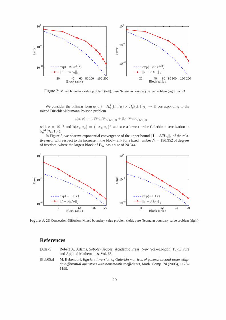
Comparing the results with our theoretical bound from Theorem 2.7, we empirically observea rate ofe−br1/2 instead ofe−br1/4 . Moreover, whether we study mixed boundary conditions orpure Neumann boundary conditions does not make any difference, as both model problems lead tosimilar computational results.

7.3 Convection-Diffusion

Finally, we study a convection-diffusion problem on the L-shaped domainΩ = (0, 1) × (0, 12 ) ∪(0, 12 ) × [ 12 , 1). The boundaryΓ = ∂Ω is divided into the Neumann partΓN := x ∈ Γ : x2 =

0 ∨ x1 = 1 and the Dirichlet partΓD = Γ\ΓN .

19

20 40 60 80 100 150 200

10−10

10−5

100

Err

or

Block rank r

exp(−2.3 r1/2)

‖I −ABH‖2

20 40 60 80 100 150 200

10−10

10−5

100

Err

or

Block rank r

‖I −ABH‖2

exp(−2.5 r1/2)

Figure 2:Mixed boundary value problem (left), pure Neumann boundary value problem (right) in 3D

We consider the bilinear forma(·, ·) : H10 (Ω,ΓD) × H1

0 (Ω,ΓD) → R corresponding to themixed Dirichlet-Neumann Poisson problem

a(u, v) := c 〈∇u,∇v〉L2(Ω) + 〈b · ∇u, v〉L2(Ω)

with c = 10−2 andb(x1, x2) = (−x2, x1)T and use a lowest order Galerkin discretization inS1,10 (Th,ΓD).

In Figure 3, we observe exponential convergence of the upper bound‖I−ABH‖2 of the rela-tive error with respect to the increase in the block-rank for a fixed numberN = 196.352 of degreesof freedom, where the largest block ofBH has a size of 24.544.

8 12 16 2010

−10

10−5

100

Err

or

Block rank r

exp(−1.08 r)

‖I −ABH‖2

8 12 16 20

10−10

10−5

100

Err

or

Block rank r

‖I −ABH‖2

exp(−1.1 r)

Figure 3:2D Convection-Diffusion: Mixed boundary value problem (left), pure Neumann boundary value problem (right).

References

[Ada75] Robert A. Adams,Sobolev spaces, Academic Press, New York-London, 1975, Pureand Applied Mathematics, Vol. 65.

[Beb05a] M. Bebendorf,Efficient inversion of Galerkin matrices of general second-order ellip-tic differential operators with nonsmooth coefficients, Math. Comp.74 (2005), 1179–1199.

20

[Beb05b] , Hierarchical LU decomposition-based preconditioners for BEM, Computing74 (2005), no. 3, 225–247.

[Beb07] , Why finite element discretizations can be factored by triangular hierarchicalmatrices, SIAM J. Numer. Anal.45 (2007), no. 4, 1472–1494.

[Beb08] , Hierarchical Matrices, Lecture Notes in Computational Science and Engi-neering, vol. 63, Springer, Berlin, 2008.

[BG99] S. Borm and L. Grasedyck,H-Lib - a library for H- andH2-matrices, available athttp://www.hlib.org, 1999.

[BH03] M. Bebendorf and W. Hackbusch,Existence ofH-matrix approximants to the inverseFE-matrix of elliptic operators withL∞-coefficients, Numer. Math.95 (2003), no. 1,1–28.

[BL04] Jeffrey K. Bennighof and R. B. Lehoucq,An automated multilevel substructuringmethod for eigenspace computation in linear elastodynamics, SIAM J. Sci. Comput.25 (2004), no. 6, 2084–2106 (electronic). MR 2086832 (2005c:74030)

[Bor10a] S. Borm,Approximation of solution operators of elliptic partial differential equationsbyH- andH2-matrices, Numer. Math.115(2010), no. 2, 165–193.

[Bor10b] , Efficient numerical methods for non-local operators, EMS Tracts in Mathe-matics, vol. 14, European Mathematical Society (EMS), Zurich, 2010.

[CDGS10] S. Chandrasekaran, P. Dewilde, M. Gu, and N. Somasunderam,On the numerical rankof the off-diagonal blocks of Schur complements of discretized elliptic PDEs, SIAM J.Matrix Anal. Appl.31 (2010), no. 5, 2261–2290. MR 2740619 (2011j:15023)

[DFG+01] W. Dahmen, B. Faermann, I. G. Graham, W. Hackbusch, and S. A. Sauter,Inverse in-equalities on non-quasiuniform meshes and application to the mortar element method,Math. Comp.73 (2001), 1107–1138.

[DKP+08] Leszek Demkowicz, Jason Kurtz, David Pardo, Maciej Paszynski, Waldemar Rachow-icz, and Adam Zdunek,Computing withhp-adaptive finite elements. Vol. 2, Chap-man & Hall/CRC Applied Mathematics and Nonlinear Science Series, Chapman &Hall/CRC, Boca Raton, FL, 2008, Frontiers: three dimensional elliptic and Maxwellproblems with applications. MR 2406401 (2009e:65172)

[EG06] Alexandre Ern and Jean-Luc Guermond,Evaluation of the condition number in linearsystems arising in finite element approximations, M2AN Math. Model. Numer. Anal.40 (2006), no. 1, 29–48.

[FMP12] M. Faustmann, J. M. Melenk, and D. Praetorius,A new proof for existence ofH-matrixapproximants to the inverse of FEM matrices: the Dirichlet problem for the Laplacian,ASC Report 51/2012, Institute for Analysis and Scientific Computing, Vienna Univer-sity of Technology, Wien (2012).

[FMP13] , Existence ofH-matrix approximation to the inverse of BEM matrices: thesimple layer operator, Tech. Report in preparation, Institute for Analysis and ScientificComputing, Vienna University of Technology, Wien, 2013.

[GGMR09] Leslie Greengard, Denis Gueyffier, Per-Gunnar Martinsson, and Vladimir Rokhlin,Fast direct solvers for integral equations in complex three-dimensional domains, ActaNumer.18 (2009), 243–275. MR 2506042 (2010e:65252)

[GH03] L. Grasedyck and W. Hackbusch,Construction and arithmetics ofH-matrices, Com-puting70 (2003), no. 4, 295–334.

[GHK08] L. Grasedyck, W. Hackbusch, and R. Kriemann,Performance ofH-LU precondition-ing for sparse matrices, Comput. Methods Appl. Math.8 (2008), no. 4, 336–349.

[Gie01] K. Giebermann,Multilevel approximation of boundary integral operators, Computing67 (2001), no. 3, 183–207. MR 1872653 (2002m:65128)

21

[GKLB08] Lars Grasedyck, Ronald Kriemann, and Sabine Le Borne, Parallel black boxH-LUpreconditioning for elliptic boundary value problems, Comput. Vis. Sci.11 (2008),no. 4-6, 273–291. MR 2425496 (2009m:65056)

[GKLB09] L. Grasedyck, R. Kriemann, and S. Le Borne,Domain decomposition basedH-LUpreconditioning, Numer. Math.112(2009), no. 4, 565–600.

[GM13] A. Gillman and P. Martinsson,A direct solver withO(N) complexity for variablecoefficient elliptic PDEs discretized via a high-order composite spectral collocationmethod, Tech. report, 2013,arXiv:1302.5995 [math.NA].

[Gra01] L. Grasedyck,Theorie und Anwendungen Hierarchischer Matrizen, doctoral thesis (inGerman), Kiel, 2001.

[Gra05] , Adaptive recompression ofH-matrices for BEM, Computing74(2005), no. 3,205–223.

[GYM12] Adrianna Gillman, Patrick M. Young, and Per-Gunnar Martinsson,A direct solver withO(N) complexity for integral equations on one-dimensional domains, Front. Math.China7 (2012), no. 2, 217–247. MR 2897703

[Hac99] W. Hackbusch,A sparse matrix arithmetic based onH-matrices. Introduction toH-matrices, Computing62 (1999), no. 2, 89–108.

[Hac09] , Hierarchische Matrizen: Algorithmen und Analysis, Springer, Dordrecht,2009.

[HB02] Wolfgang Hackbusch and Steffen Borm,H2-matrix approximation of integral opera-tors by interpolation, Appl. Numer. Math.43 (2002), no. 1-2, 129–143, 19th DundeeBiennial Conference on Numerical Analysis (2001). MR 1936106

[HG12] Kenneth L. Ho and Leslie Greengard,A fast direct solver for structured linear systemsby recursive skeletonization, SIAM J. Sci. Comput.34 (2012), no. 5, A2507–A2532.MR 3023714

[HJ13] Roger A. Horn and Charles R. Johnson,Matrix analysis, second ed., Cambridge Uni-versity Press, Cambridge, 2013. MR 2978290

[HKS00] W. Hackbusch, B. Khoromskij, and S. A. Sauter,On H2-matrices, Lectures on ap-plied mathematics (Munich, 1999), Springer, Berlin, 2000, pp. 9–29. MR 1767761(2001f:65034)

[HY13] K.L. Ho and L. Ying, Hierarchical interpolative factorization for elliptic operators:differential equations, Tech. report, 2013,arXiv:1307.2895 [math.NA].

[KS99] G.E. Karniadakis and S.J. Sherwin,Spectral/hp element methods for cfd, Oxford Uni-versity Press, 1999.

[LBG06] Sabine Le Borne and Lars Grasedyck,H-matrix preconditioners in convection-dominated problems, SIAM J. Matrix Anal. Appl.27 (2006), no. 4, 1172–1183 (elec-tronic). MR 2205618 (2007d:65033)

[LGWX12] Shengguo Li, Ming Gu, Cinna Julie Wu, and Jianlin Xia,New efficient and robust HSSCholesky factorization of SPD matrices, SIAM J. Matrix Anal. Appl.33 (2012), no. 3,886–904. MR 3023456

[Lin04] M. Lintner, The eigenvalue problem for the 2D Laplacian inH- matrix arithmetic andapplication to the heat and wave equation, Computing72 (2004), no. 3-4, 293–323.

[Mar09] Per-Gunnar Martinsson,A fast direct solver for a class of elliptic partial differentialequations, J. Sci. Comput.38 (2009), no. 3, 316–330. MR 2475654 (2010c:65041)

[Sch98] Ch. Schwab,p- andhp-finite element methods, Numerical Mathematics and ScientificComputation, The Clarendon Press Oxford University Press, New York, 1998, Theoryand applications in solid and fluid mechanics.

[Sch06] R. Schreittmiller,Zur Approximation der Losungen elliptischer Systeme partieller Dif-ferentialgleichungen mittels Finiter Elemente undH-Matrizen, Ph.D. thesis, Technis-che Universitat Munchen, 2006.

22

[SY12] Phillip G. Schmitz and Lexing Ying,A fast direct solver for elliptic problems on gen-eral meshes in 2D, J. Comput. Phys.231(2012), no. 4, 1314–1338. MR 2876456

[SZ90] L. R. Scott and S. Zhang,Finite element interpolation of nonsmooth functions satisfy-ing boundary conditions, Math. Comp.54 (1990), no. 190, 483–493.

[XCGL09] Jianlin Xia, Shivkumar Chandrasekaran, Ming Gu, and Xiaoye S. Li,Superfast multi-frontal method for large structured linear systems of equations, SIAM J. Matrix Anal.Appl. 31 (2009), no. 3, 1382–1411. MR 2587783 (2011c:65072)

[Xia13] Jianlin Xia,Efficient structured multifrontal factorization for general large sparse ma-trices, SIAM J. Sci. Comput.35 (2013), no. 2, A832–A860. MR 3035488

23