complexity and approximability of the cover polynomial filecomplexity and approximability
TRANSCRIPT

COMPLEXITY AND APPROXIMABILITY
OF THE COVER POLYNOMIAL
Markus Blaser, Holger Dell, and Mahmoud Fouz
Abstract. The cover polynomial and its geometric version intro-duced by Chung & Graham and D’Antona & Munarini, respectively,are two-variate graph polynomials for directed graphs. They count the(weighted) number of ways to cover a graph with disjoint directed cyclesand paths, they can be thought of as interpolations between determi-nant and permanent, and are proposed as directed analogues of the Tuttepolynomial.Jaeger, Vertigan, and Welsh showed that the Tutte polynomial is #P-hard to evaluate at all but a few special points and curves. It turns outthat the same holds for the cover polynomials: We prove that, in almostthe whole plane, the problem of evaluating the cover polynomial andits geometric version is #P-hard under polynomial-time Turing reduc-tions, while only three points in the cover polynomial and two points inthe geometric cover polynomial are easy. We also study the complex-ity of approximately evaluating the geometric cover polynomial. Underthe reasonable complexity assumptions RP 6= NP and RFP 6= #P,we give a succinct characterization of a large class of points at whichapproximating the geometric cover polynomial within any polynomialfactor is not possible.
Keywords. Graph Polynomial, Counting Complexity, Approximation,Permanent, Tutte Polynomial
Subject classification. 68Q17, 05C99
1. Introduction
Graph polynomials map directed or undirected graphs to polynomials in one ormore variables, such that this mapping is invariant under graph isomorphisms.Probably the most famous graph polynomials are the chromatic polynomialor its generalization, the Tutte polynomial. The chromatic polynomial is thepolynomial in the variable λ that counts the number of valid λ-colourings of a
2 Blaser, Dell & Fouz
given undirected graph. The Tutte polynomial T in two variables x and y hasinterpretations from different fields of combinatorics. For example, T (G; 1, 1) isthe number of spanning trees, T (G; 1, 2) is the number of spanning subgraphsof an undirected graph G, and also the number of nowhere-zero flows or theJones polynomial of an alternating link are contained in the Tutte polynomial.
While the Tutte polynomial has been established for undirected graphs,the cover polynomial by Chung & Graham (1995) and its geometric versionby D’Antona & Munarini (2000) are analogues for the directed case. Both theTutte and the cover polynomials satisfy similar identities such as a contraction-deletion identity and product rule, but the exact relation between the Tutteand the cover polynomials is not yet known. The cover polynomials haveconnections to rook polynomials and drop polynomials, but from a complexitytheoretic point of view, we tend to see them as generalizations of the permanentand the determinant of a graph. The cover polynomials of a graph are weightedsums of all of its spanning subgraphs that consist of disjoint, directed, andsimple cycles and paths. As it is the case for most graph polynomials, the coverpolynomials are of interest because they combine a variety of combinatorialproblems into one generalized theoretical framework.
Previous Results. Jaeger et al. (1990) proved that, except along one hyper-bola and at nine special points, computing the Tutte polynomial is #P-hard.For the chromatic polynomial, a substitution instance of the Tutte polynomial,this was shown first by Linial (1986). In recent years, the complexity and ap-proximability of the Tutte polynomial has received increasing attention: Lotz& Makowsky (2004) proved that the coloured Tutte polynomial by Bollobas& Riordan (1999) is complete for Valiant’s algebraic complexity class VNP,Gimenez & Noy (2006) showed that evaluating the Tutte polynomial is #P-hard even for the rather restricted class of bicircular matroids, and Goldberg& Jerrum (2008) show that the Tutte polynomial is inapproximable in largeregions of the Tutte plane.
A different graph invariant that is related to the Tutte polynomial is theweighted sum of graph homomorphisms to a fixed graph H , so basically, it is thenumber of H-colourings. Bulatov & Grohe (2005) and Dyer et al. (2006) provedthat the complexity of computing this sum is #P-hard for most graphs H .
Recently, results similar to ours have been shown for many other graphpolynomials. For instance, Hoffmann (2010) proved that the edge elimina-tion polynomial defined by Averbouch et al. (2008) is #P-hard to evaluatealmost everywhere. Blaser & Hoffmann (2008) showed that the interlace poly-nomial is #P-hard to evaluate except for a finite number of lines. Blaser et al.
Complexity and Approximability of the Cover Polynomial 3
(2008) extended the results by Jaeger, Vertigan, and Welsh to the colored Tuttepolynomial. More importantly, they introduce algebraic reductions which givestronger hardness results: Evaluation at almost all points are not just shownto be hard but the evaluation at almost all points can be reduced to the evalu-ation at any other of these points. Makowsky (2008), in his so-called “difficultpoint conjecture”, conjectures that this is a general phenomenon: Every poly-nomial that is definable in monadic second order logic is #P-hard to evaluatealmost everwhere provided it has at least one hard point. Many of the graphpolynomials studied in the literature are definable in monadic second orderlogic.
Courcelle et al. (2001) established the result that every graph polynomialthat is definable in monadic second order logic is linear time computable ongraphs with bounded treewidth. The dependence of the running time on thetreewidth is usually very high. But it is often possible to obtain better algo-rithms for specific graph polynomial by exploiting their particular properties,for instance by Noble (1998) and Andrzejak (1998) for the Tutte polynomialor by Blaser & Hoffmann (2009) for the interlace polynomial. For generalgraphs, Bjorklund et al. (2008) proved that Tutte polynomials as well as thecover polynomials can be computed in vertex-exponential time, that is, in time2O(n) poly(n) where n is the number of vertices.
Our Contribution. In this paper, we show that the problem of evaluatingthe cover polynomial and its geometric version is #P-hard at all evaluationpoints except for three and two points, respectively, where this is easy. More-over, we prove that, under reasonable complexity assumptions, there is nofully polynomial randomized approximation scheme (FPRAS) for the geomet-ric cover polynomial at all rational points (x, y) ∈ Q2 that have the followingproperty: there exists a graph D s.t. C(D; x, y) = 0. The only exceptions arethree special points that are either polynomially computable or approximableand a half-line whose approximability is unknown. Interestingly, this class ofinapproximable points turns out to exhibit different levels of intractability. Atsome points, like those on the positive y-axis, there exists an FPRAS for thegeometric cover polynomial using an oracle for an NP predicate. In contrast,there are points at which approximating the geometric cover polynomial is ashard as its exact computation. In addition, we will extend some of these resultsto the cover polynomial by Chung and Graham.
Our main techniques for the #P-hardness proofs are gadgets and interpola-tion. Most notably, we present an elegant gadget that generalizes and simplifiesthe XOR-gadget by Valiant (1979). Since interpolation is not approximation-
4 Blaser, Dell & Fouz
preserving in general, the gadgets for the inapproximability proofs are moreinvolved, and they are used in the reductions to amplify intractable informa-tion contained in the cover polynomial.
2. Preliminaries
Let N = {0, 1, . . .}. The graphs in this paper are directed multigraphs D =(V, E) with parallel edges and loops allowed. We denote by G the set of allsuch graphs. We write n for the number of vertices, and m for the number ofedges. Two graphs are called isomorphic if there is a bijective mapping on thevertices that transforms one graph into the other.
A graph invariant is a function f : G → F , mapping elements from G tosome set F , such that all pairs of isomorphic graphs G and G′ have the sameimage under f . In the case that F is a polynomial ring, f is called graphpolynomial.
Counting Complexity Basics. Let Σ = {0, 1}. The class #P consists ofall functions f : Σ∗ → N for which there is a non-deterministic polynomial-time bounded Turing machine M which has exactly f(x) accepting paths oninput x. We can extend #P to include functions over the rationals that are notharder to compute than counting problems in #P. Specifically, we define #PQ
as the class of all mappings f : Σ∗ → Q, such that f = ab, where a : Σ∗ → N
and b : Σ∗ → Q are counting problems with a ∈ #P and b ∈ FP. Here, FP isthe class of polynomially computable functions.
For two counting problems f, g : Σ∗ → Q, we say f Turing-reduces to gin polynomial time (f 4p
T g), if there is a deterministic oracle Turing machinewhich computes f in polynomial time with oracle access to g. If the oracle isused only once, we say f many-one reduces to g (f 4p
m g), and if the oracleoutput is the output of the reduction, we speak of a parsimonious many-onereduction (f 4p g). The notions of #P-hardness and #P-completeness (underpolynomial-time Turing reductions) are defined in the usual way. We willmainly use Turing reductions in our work. Of course, it would be desirable toget hardness results under many-one or even parsimonious reductions; however,we need interpolation to construct our reductions.
Although we formulate our reductions in terms of Turing-reductions over Qwhich is represented as strings over a binary alphabet, they are actually of auniformly algebraic nature. In particular, they can be transferred effortlesslyto, say, the BSS-model over R or C (cf. Blum et al. (1998)). “Algebraic nature”essentially means that our reductions map graphs to graphs (via polynomialtime computable functions) and points to points (via rational functions).
Complexity and Approximability of the Cover Polynomial 5
Approximability Basics. For many optimization problems f : Σ∗ → Q, nopolynomial time algorithm is known to compute f exactly. Still, in many cases,there exist algorithms that compute the value of f approximately. In somesense, the best one can hope for in these cases is a fully polynomial randomizedapproximation scheme (FPRAS). A randomized approximation scheme for f isa randomized algorithm that takes as input, besides the instance x ∈ Σ∗, anerror parameter ǫ > 0, and outputs a number z ∈ Q such that
(2.1) Pr[
|f(x) − z| ≤ ǫ |f(x)|]
≥ 34.
It is said to be a fully polynomial randomized approximation scheme if itsrunning time is bounded by a polynomial in |x| and ǫ−1.
An interesting result (Valiant & Vazirani 1986, Corollary 3.6) states that#3Sat has an FPRAS that uses an oracle to an NP predicate. Since anyproblem in #P can be parsimoniously reduced to #3Sat (see Papadimitriou(1994) for details), we get the following corollary.
Corollary 2.2. If f ∈ #PQ, then there exists an FPRAS for f using anoracle to an NP predicate.
Proof. Let f = ab
with a ∈ #P and b ∈ FP. Given input x, reduce xparsimoniously to an instance y of #3Sat. Apply the #3Sat-FPRAS withoracle access to the NP-predicate to y. Divide the result by b(x). �
Parsimonious reductions from f to g are particularly useful as they allowthe transformation of an FPRAS for g into an FPRAS for f . They are approx-imation preserving. In general, a Turing reduction from f to g is said to beapproximation preserving if it provides a c-approximation (i.e., an approximateresult that is at most a factor of c away from the exact result) for f wheneverthe oracle is replaced by a c-approximation algorithm for g. If f can be reducedto g via an approximation preserving reduction, we write f ≤AP g. From thedefinition, we get the following easy, but useful fact.
Fact 2.3. Let f, g : Σ∗ → Q. If f ≤AP g and there exists an FPRAS for g,then there also exists an FPRAS for f .
What if there exists no FPRAS for a function f? Can we still hope for arandomized approximation algorithm that yields, say, constant factor approx-imations for f(x)? A surprising result states that this is not possible for acommon class of problems, namely, self-reducible problems. We call a function
6 Blaser, Dell & Fouz
f self-reducible, if it can be evaluated by a deterministic polynomial time ora-cle Turing machine with oracle access to f that is only allowed to query oraclestrings of length less than the input length. Specifically, Jerrum & Sinclair(1989) prove the following ‘all-or-nothing’ theorem.
Theorem 2.4 (Jerrum and Sinclair). For a self-reducible function f : Σ∗ →Q, if there is a polynomial time randomized algorithm for computing f withina factor of poly(|x|), then there is also an FPRAS for f .
We define RFP to be the class of all functions computable by a BPP-machine, i.e., computable in polynomial time with error probability smallerthan 1
4.
When can we rule out the existence of an FPRAS for a counting problem f?The following lemma shows that, under the complexity assumption RP 6= NP,no counting version of an NP-complete problem can have an FPRAS.
Lemma 2.5. Let f : Σ∗ → N be a counting problem so that the associateddecision problem L = {x : f(x) > 0} is NP-complete.
Then there exists no FPRAS for f unless RP = NP.
Proof. An FPRAS for f would directly entail NP ⊆ BPP. It is wellknown (see, e.g., (Papadimitriou 1994, Problem 11.5.18)) that the latter impliesRP = NP. �
Polynomials. Polynomials p(x1, . . . , xm) are elements of the polynomial ringQ[x1, . . . , xm], and, in this context, the variables are abstract objects. Anyunivariate polynomial can be interpolated if sufficiently many point-value pairsare known. For multivariate polynomials, this is not always true since thepoints must be positioned, say, in a grid. However, it is sufficient for us thatthe following univariate interpolation problem can be solved in polynomial timeusing Lagrange interpolation (where m = 1):Input: Point-value pairs (a0, p0), . . . , (ad, pd) ∈ Q2, encoded in binary.Output: The coefficients of the polynomial p(x) with deg(p) ≤ d and p(aj) = pj .Note that interpolation is not approximation preserving in general.
Path-Cycle Decompositions. The cover polynomials basically count a re-laxed form of cycle covers, namely path-cycle covers or path-cycle decomposi-tions. For a directed graph D = (V, E) and some subset PC ⊆ E, we denote thesubgraph (V,PC) again by PC. A path-cycle cover of D is a set PC ⊆ E, suchthat, in PC, every vertex v ∈ V has an indegree and an outdegree of at most 1.A path-cycle cover thus consists of disjoint simple paths and simple cycles.
Complexity and Approximability of the Cover Polynomial 7
Note that also an independent vertex counts as a path, and an independentloop counts as a cycle.
We write ρ(PC) and σ(PC) for the number of paths and cycles of a path-cycledecomposition PC. By the graph invariant cD(ρ, σ), we denote the number ofpath-cycle covers of D that have exactly ρ paths and σ cycles. It is not hard toprove that the function D 7→ cD(ρ, σ) is #P-complete: Counting Hamiltonianpaths or cycles is #P-complete, that is cD(0, 1) and cD(1, 0) is #P-complete.We can reduce the computation of these two coefficients to the computation ofcD(ρ, σ) by adding an appropriate number of independent vertices and/or selfloops.
Cover Polynomials. We consider two variants of the cover polynomial: Theoriginal factorial cover polynomial defined by Chung & Graham (1995), andthe more intuitive version by D’Antona & Munarini (2000).
The factorial cover polynomial or Chung-Graham polynomial is a graphpolynomial in the variables x and y, and it is defined by
(2.6) Cfac(D; x, y) :=
n∑
ρ=0
m∑
σ=0
cD(ρ, σ)xρyσ,
where xρ := x(x − 1) . . . (x − ρ + 1) denotes the falling factorial. The Chung-Graham polynomial can also be written as a weighted sum over all covers of D:
Cfac(D; x, y) =∑
path-cyclecover PC
xρ(PC)yσ(PC).
The geometric cover polynomial or D’Antona-Munarini polynomial is agraph polynomial Cgeo(D; x, y) defined in a similar manner as the Chung-Graham polynomial, except that the falling factorial xρ is replaced with a usualpower xρ. When clear from the context, we may use the notation C(D; x, y)for both versions of the cover polynomial.
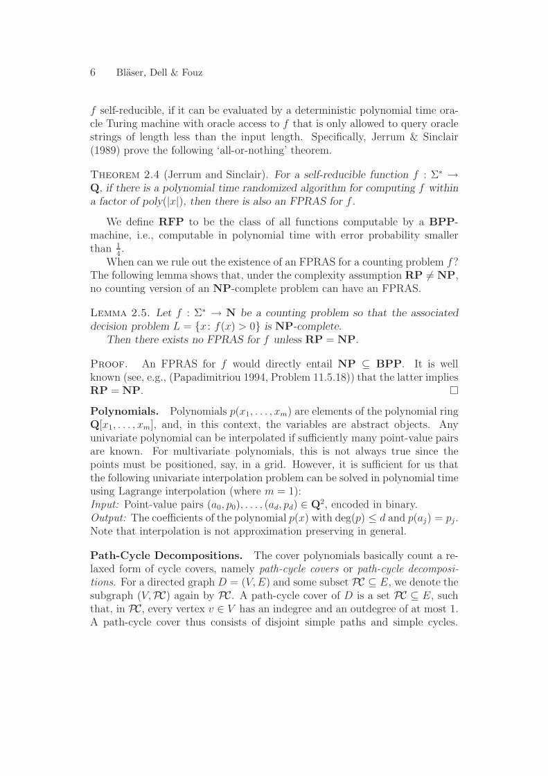
Contraction-Deletion Identity. By D \ e, we denote the deletion, andby D/e, the contraction of an edge e. If e is incident to u and v, then D/e isobtained from D by merging u and v, and by removing all edges that either startat u or end in v (this directed contraction is different from a usual undirectedcontraction, see Figure 2.1). If e is a loop then the convention is to completelyremove the corresponding vertex when contracting e. An alternative way todefine the cover polynomial C(D) = C(D; x, y) is by a contraction-deletion
8 Blaser, Dell & Fouz
e
Figure 2.1: Directed contraction. The edge e is contracted. Two edges areremoved, because they would create a path in the new graph that is not presentin the original graph.
identity:
(2.7) C(D) =
C(D \ e) + C(D/e) if e is not a loop in D,
C(D \ e) + yC(D/e) if e is a loop in D,
xn or xn if there is no edge in D.
In this recursion, C(D \ e) counts those path-cycle covers that do not use ewhile C(D/e) counts the others. This way, every cycle shrinks to a loop andthen vanishes, contributing a weight of y.
Using these identities, it is easy to see that, just like the Tutte polynomial,the geometric cover polynomial has a very useful product rule.
Lemma 2.8. Let D1,2 be the disjoint union of two digraphs D1 and D2. Forall x, y ∈ Q, we have
Cgeo(D1,2; x, y) = Cgeo(D1; x, y)Cgeo(D2; x, y).
3. Results
Our focus is to study the computational problem of evaluating the cover poly-nomials at fixed evaluation points (x, y) ∈ Q2. By abuse of notation, we denoteby C(x, y) the graph parameter C( . , x, y), i.e., x and y are fixed and the inputsare digraphs D.
Name C(x, y).
Instance Digraph D = (V, E).
Output C(D; x, y).
Complexity and Approximability of the Cover Polynomial 9
1
1
x
y
Permanent
Determinant
4p
T
4p T
4p
T
#Hamiltonian
Paths
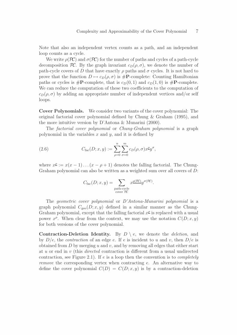
Figure 3.1: The Chung-Graham plane: three points (black discs) are easy toevaluate, and the rest of the plane is #P-hard. The crosses indicate the pointsfor the reductions.
Formally, C(x, y) is the function from G → Q with D 7→ C(D; x, y) wherewe assume graphs and rationals to be represented explicitly over a binary al-phabet in a reasonable way. For both cover polynomials, we give a dichotomytheorem on the computational complexity of exact evaluation.
Theorem 3.1. The evaluations C(0, 0), C(0,−1), and Cfac(1,−1) are com-putable in polynomial time.
All other evaluations Cgeo(x, y) and Cfac(x, y) are #P-hard.
Proof (outline). The proof is in several steps (cf. Figure 3.1). We begin byclassifying the polynomial-time computable points in Section 4.1. Furthermore,we point out that Cfac(0, 1) is the permanent and Cfac(1, 0) is the number ofHamiltonian paths, which both are #P-complete counting problems.
In Section 4.2, using elementary identities of the cover polynomial and in-terpolation, we reduce along horizontal lines, that means we prove Cfac(0, y) 4p
T
Cfac(x, y) for all x, y and Cfac(1, 0) 4pT Cfac(x, 0) for all x 6= 0. This implies the
hardness of Cfac(x, 1) for all x and of Cfac(x, 0) for x 6= 0.To prove the remaining hardness part where y 6∈ {−1, 0, 1}, we reduce the
permanent to Cfac(0, y). Section Section 4.3 is the core part of our proof,establishing this reduction Cfac(0, 1) 4p
T Cfac(0, y) along the y-axis. There weintroduce and analyze the equality gadget, use it to establish a new identity
10 Blaser, Dell & Fouz
for the weighted cover polynomial, and show how to derive a reduction for thestandard cover polynomial from this.
In Section 4.4, we show how to carry over our result to the geometric versionof the cover polynomial. �
Remark 3.2. It is easily verified that all the reductions that we use are al-gebraic, as defined in Blaser et al. (2008). Furthermore, we can reduce theevaluation at almost every point (x′, y′) to almost every other point uniformly:First we reduce C(x′, y′) to C(0, y′) using horizontal reductions and interpola-tion, then we reduce C(0, y′) to C(0, y) using the vertical reduction, and thenfinally reducing C(0, y) to C(x, y).
In the second part of this article, we analyze the inapproximability of thegeometric cover polynomial. We say that (x, y) ∈ Q2 has a root if there existsa graph D such that Cgeo(D; x, y) = 0.
Theorem 3.3. Let (x, y) ∈ Q2 \{
(0, 0), (0,−1)}
. The following holds.
◦ If x ≥ 0 and y = 1, then there exists an FPRAS for Cgeo(x, y).
◦ If 1 6= y > 0 and (x, y) has a root, then Cgeo(x, y) cannot be approximatedwithin any polynomial factor unless RP = NP.
◦ If y ≤ 0 and (x, y) has a root, then Cgeo(x, y) cannot be approximatedwithin any polynomial factor unless RFP = #P.
Although we also have some results on the inapproximability of the factorialcover polynomial, they are not as nice as the theorem above, so we postponesuch a theorem to the end of the article. The reason why it seems much moredifficult to handle the factorial cover polynomial lies in the fact that in contrastto the geometric version, it lacks a proper product rule. As a result the gadgetsdesigned for the geometric cover polynomial fail for the factorial version. Ofcourse, we can obtain the factorial cover polynomial from the geometric coverpolynomial by a change of basis and vice versa. For this, we need the coefficientsof the polynomial which we can compute using interpolation. However, whenwe consider approximability, we do not get exact values but only very crudeapproximations to it. There is no hope of obtaining useful results by usingthese approximations for interpolation.
Complexity and Approximability of the Cover Polynomial 11
4. Complexity of the Cover Polynomial
4.1. Special Points. A Hamiltonian path is a path-cycle cover with exactlyone path and zero cycles, and a cycle cover is a path-cycle cover without paths.The permanent Perm(D) is the permanent of the adjacency matrix A of D,and it equals the number of cycle covers of D. The determinant det(D) is thedeterminant det(A). Remarkably, both the determinant and the permanentcan be found in the cover polynomial.
Lemma 4.1. Let D be a directed nonempty graph.We have
(i) Cfac(D; 0, 0) = 0,
(ii) Cfac(D; 1, 0) = #HamiltonianPaths(D),
(iii) Cfac(D; 0, 1) = Perm(D),
(iv) Cfac(D; 0,−1) = (−1)n det(D),
(v) Cfac(D; 1,−1) = Cfac(D; 0,−1) − Cfac(D′; 0,−1) where D′ is a graph de-
rived from D by adding an apex v0, that is, a fresh node and all edges toand from the nodes of D.
Proof. The proof of the first three claims is simple.(i) Note that the empty graph E0 = (∅, ∅) is the only graph that can be
path-cycle covered without any paths or cycles, and that there is exactly onesuch cover. Because of 0ρ0σ = 1 if and only if ρ = σ = 0, we have
C(D; 0, 0) =∑
ρ,σ
cD(ρ, σ)0ρ0σ = cD(0, 0) = 0.
(ii) Using 1ρ0σ = 1 if and only if ρ ∈ {0, 1} ∧ σ = 0, we get
C(D; 1, 0) =∑
ρ,c
cD(ρ, σ)1ρ0σ = cD(0, 0) + cD(1, 0)
= #HamiltonianPaths(D).
(iii) The property 0ρ1σ = 1 if and only if ρ = 0 reveals
C(D; 0, 1) =∑
ρ,σ
cD(ρ, σ)0ρ1σ =∑
σ
cD(0, σ) = Perm(D).

12 Blaser, Dell & Fouz
(iv) For the fourth claim, recall the Leibniz formula for the determinant:
det(D) =∑
π∈Sn
sgn(π)∏
i
Aiπ(i).
The permutations π with∏
i Aiπ(i) 6= 0 stand in bijection with the cycle cov-ers C of D. For a cyclic permutation τ of length ℓ, sgn(τ) = (−1)ℓ+1. Thus,sgn(π) = (−1)n+σ(C) holds for each permutation π and its corresponding cyclecover C with σ(C) cycles.
(v) For the last claim, notice that C(D; 1,−1) counts all path-cycle cov-ers with at most one path (weighted with (−1)σ(C)), while the determinantC(D; 0,−1) counts only cycle covers. The idea is that C(D; 1,−1)−C(D; 0,−1)is the number of covers of D with exactly one path, and can be expressed byC(D′; 0,−1), the number of cycle covers of D′. This is because every path-cycle cover of D with one path becomes a cycle cover in D′ where the path getsclosed by taking a detour through the apex v0 to form a cycle.
Let D′ be the graph obtained from D by adding one additional fresh ver-tex v0 to it, and by adding the edges (v0, v) and (v, v0) for every vertex v of D.We claim that, for all 0 6= y ∈ Q, we have
C(D; 1, y) = C(D; 0, y) + y−1C(D′; 0, y).
First we notice that cD′(0, σ) = cD(1, σ − 1) for all σ > 0: Every cycle cover C′
of D′ with σ cycles uses two edges (v0, u) and (v, v0). If we remove these twoedges, we get a path-cycle cover PC of D where the cycle that went throughv0 is broken up into a path from u to v. This means that PC uses exactly onepath and it uses one cycle less than C′. On the other hand, assume that PCis a path-cycle cover of D with σ − 1 cycles and 1 path. Assume the path isfrom u to v. By adding the edges (v0, u) and (v, v0), we get a cycle cover of D′.Thus, there is a suitable bijection which implies cD′(0, σ) = cD(1, σ − 1).
Now we note that 0ρ = 1 if and only if ρ = 0, and 1ρ = 1 if and only ifρ = 0, 1. And we note that D′ is nonempty, such that cD′(0, 0) = 0. Then we

Complexity and Approximability of the Cover Polynomial 13
b b′
a′
a
D
v v′
ev
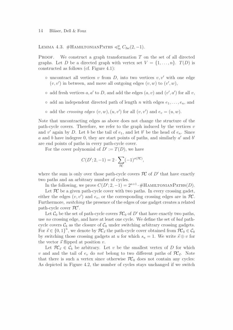
Figure 4.1: Shows the graph D′ :=T (D) constructed in the proof ofLemma 4.3. The two edges ev, (v, v′)together with the corresponding cross-ing edges form the crossing gadget.
Figure 4.2: Shows the change in thenumber of paths and cycles in a path-cycle cover if we switch one crossinggadget.
can verify the following computation.
C(D; 1, y)
=∑
ρ,σ≥0
1ρyσcD(ρ, σ) by definition
=∑
σ≥0
yσcD(0, σ) +∑
σ≥0
yσcD(1, σ) because 1ρ = [ρ = 0 or ρ = 1]
= C(D; 0, y) +∑
σ≥0
yσcD′(0, σ + 1) from cD′(0, σ) = cD(1, σ − 1)
= C(D; 0, y) +∑
σ≥1
yσ−1cD′(0, σ) index transformation
= C(D; 0, y) + y−1∑
σ≥0
yσcD′(0, σ) because cD′(0, 0) = 0
= C(D; 0, y) + y−1C(D′; 0, y). �
Corollary 4.2. (i) Cfac(1, 0) and C(0, 1) are #P-complete.
(ii) C(0, 0), C(0,−1), and Cfac(1,−1) are polynomial-time computable.
Proof. The first item follows from the results of Dyer et al. (1998) andValiant (1979), respectively. C(0, 0) is trivial and for the other two points, wecan use Gaussian elimination. �
The #P-hardness of Cfac(2,−1) follows from the following lemma.
14 Blaser, Dell & Fouz
Lemma 4.3. #HamiltonianPaths 4pm Cfac(2,−1).
Proof. We construct a graph transformation T on the set of all directedgraphs. Let D be a directed graph with vertex set V = {1, . . . , n}. T (D) isconstructed as follows (cf. Figure 4.1):
◦ uncontract all vertices v from D, into two vertices v, v′ with one edge(v, v′) in between, and move all outgoing edges (v, w) to (v′, w),
◦ add fresh vertices a, a′ to D, and add the edges (a, v) and (v′, a′) for all v,
◦ add an independent directed path of length n with edges e1, . . . , en, and
◦ add the crossing edges (v, w), (u, v′) for all (v, v′) and ev = (u, w).
Note that uncontracting edges as above does not change the structure of thepath-cycle covers. Therefore, we refer to the graph induced by the vertices vand v′ again by D. Let b be the tail of e1, and let b′ be the head of en. Sincea and b have indegree 0, they are start points of paths, and similarly a′ and b′
are end points of paths in every path-cycle cover.For the cover polynomial of D′ := T (D), we have
C(D′; 2,−1) = 2 ·∑
PC
(−1)σ(PC),
where the sum is only over those path-cycle covers PC of D′ that have exactlytwo paths and an arbitrary number of cycles.
In the following, we prove C(D′; 2,−1) = 2n+1 ·#HamiltonianPaths(D).Let PC be a given path-cycle cover with two paths. In every crossing gadet,
either the edges (v, v′) and ev, or the corresponding crossing edges are in PC.Furthermore, switching the presence of the edges of one gadget creates a relatedpath-cycle cover PC′.
Let C0 be the set of path-cycle covers PC0 of D′ that have exactly two paths,use no crossing edge, and have at least one cycle. We define the set of bad path-cycle covers Cb as the closure of C0 under switching arbitrary crossing gadgets.For ~s ∈ {0, 1}n, we denote by PC~s the path-cycle cover obtained from PC0 ∈ C0
by switching those crossing gadgets at u for which su = 1. We write ~s ⊕ v forthe vector ~s flipped at position v.
Let PC~s ∈ Cb be arbitrary. Let v be the smallest vertex of D for whichv and and the tail of ev do not belong to two different paths of PC~s. Notethat there is such a vertex since otherwise PC0 does not contain any cycles:As depicted in Figure 4.2, the number of cycles stays unchanged if we switch
Complexity and Approximability of the Cover Polynomial 15
crossing gadgets that are involved in two different paths. Further note that thenumbers of cycles in PC~s and PC~s⊕v differ by exactly 1. This implies
∑
PC∈Cb
(−1)σ(PC) =∑
PC0∈C0
∑
~s
(−1)σ(PC~s) = 0,
since all terms (−1)σ(PC~s) + (−1)σ(PC~s⊕v) = 0 cancel out.
As a result, C(D′; 2,−1) is just 2 times the number of path covers of D′ withexactly two paths. Any such 2-path cover PC of D′ translates to an Hamiltonianpath of D (by switching all gadgets to PC0, recontracting the edges (v, v′), andremoving a, a′ and the b-b′-path), and this procedure does not add any cycles.Since there are 2n possible gadget states, we get
C(D′; 2,−1) = 2 · 2n · #HamiltonianPaths(D). �
4.2. Horizontal Reductions. Let us consider reductions along the horizon-tal lines Ly := {(x, y) : x ∈ Q}. For a directed graph D, let D(r) be the graphobtained by adding r independent vertices. Corollary 4 in Chung & Graham(1995) is the core part of the horizontal-line reductions:
(4.4) Cfac(D(r); x, y) = xrCfac(D; x − r, y).
From this equation, a simple interpolation argument yields the following re-duction.
Lemma 4.5. For all (x, y) ∈ Q2, we have Cfac(0, y) 4pT Cfac(x, y).
Proof. For x ∈ N, it follows directly because C(D; 0, y) = C(D(x); y, x)/xx.
For x 6∈ N, we can compute the values C(D; x − 1, y), . . . , C(D; x − m, y)using the above identity. Since C(D; x, b) is a polynomial in x of degree atmost m, this is enough to compute the coefficients of the polynomial exactlyand in polynomial time. �
In a similar fashion, one can also prove C(1, 0) 4pT C(x, 0) for x 6= 0 and
C(2,−1) 4pT C(x, 0) for x 6= 0, 1 from (4.4). Please note that, together with
Lemma 4.1, we obtain that C(x, y) is #P-hard for every point (x, y) on the linesL1, L0, and L−1, except for the three easy points (0, 0), (0,−1), and (1,−1).
4.3. Vertical Reduction. In this section, we reduce the permanent alongthe y-axis, as made explicit in the following theorem.
16 Blaser, Dell & Fouz
Theorem 4.6. Let y ∈ Q with −1 6= y 6= 0. Then C(0, 1) 4pT C(0, y).
Proof (outline). For some input graph D, we compute C(D; 0, 1) with oracleaccess to C(0, y), and we use interpolation to do so.
In order to interpolate the polynomial C(D; 0, y), we need to compute somevalues C(D; 0, y1), . . . , C(D; 0, ym). This can be done by using the oracle forsome values C(D1; 0, y), . . . , C(Dm; 0, y) instead. More specifically, we con-struct graphs Dα containing α copies of a graph D, such that there is a sim-ple relation between C(D; 0, yα) and C(Dα; 0, y). Computing C(D; 0, yα) forα = 1, . . . , m and applying interpolation, we get the coefficients of C(D; 0, y).
Construction details are spelled out in the remainder of this section. �
The constructed graph Dα is a graph in which every cycle cover ideally has αtimes the number of cycles a corresponding cycle cover of D would have. Thisway, the terms yc in the cover polynomial ideally become yαc, and some easilycomputable relation between C(D; 0, yα) and C(Dα; 0, y) can be established.
In the construction, we duplicate the graph α times, and we connect theduplicates by equality gadgets. These equality gadgets make sure that everycycle cover of Dα is a cycle cover of D copied α times, and thus has roughly αtimes the number of cycles. Let us construct the graph Dα explicitly.
◦ Start with the input graph D.
◦ Create α copies D1, . . . , Dα of D.
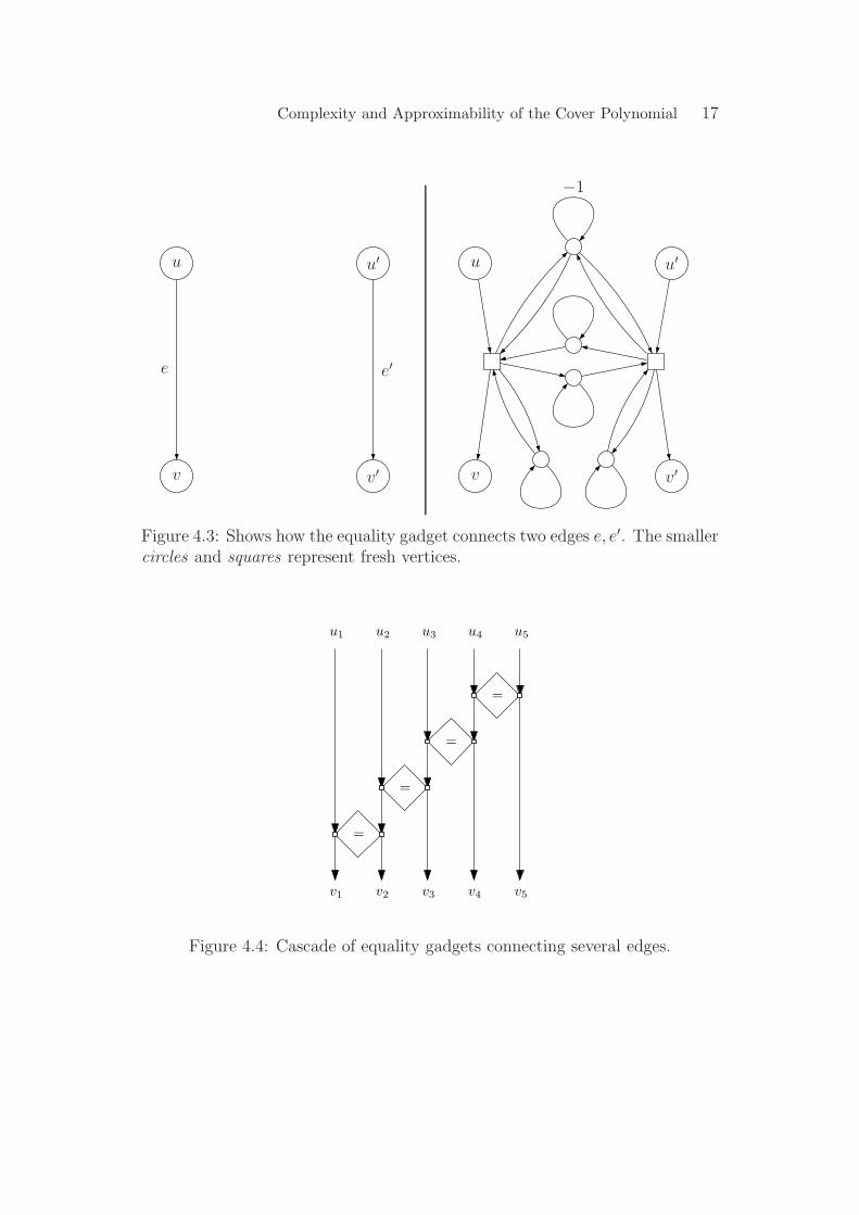
◦ Let ei be the copy of e in the graph Di. Replace every tuple of edges(e1, . . . , eα) by a cascade of equality gadgets on α edges, which is depictedin Figure 4.4.
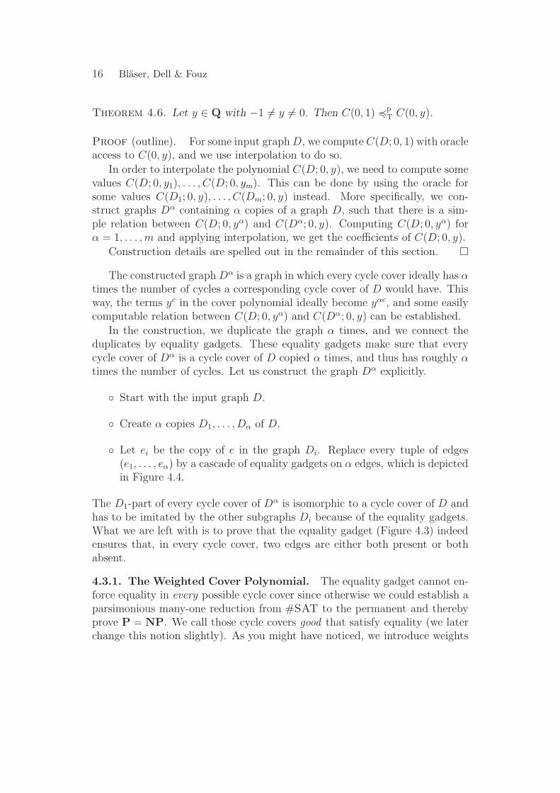
The D1-part of every cycle cover of Dα is isomorphic to a cycle cover of D andhas to be imitated by the other subgraphs Di because of the equality gadgets.What we are left with is to prove that the equality gadget (Figure 4.3) indeedensures that, in every cycle cover, two edges are either both present or bothabsent.
4.3.1. The Weighted Cover Polynomial. The equality gadget cannot en-force equality in every possible cycle cover since otherwise we could establish aparsimonious many-one reduction from #SAT to the permanent and therebyprove P = NP. We call those cycle covers good that satisfy equality (we laterchange this notion slightly). As you might have noticed, we introduce weights
Complexity and Approximability of the Cover Polynomial 17
u
v
u′
v′
e′e
u
v
u′
v′
−1
Figure 4.3: Shows how the equality gadget connects two edges e, e′. The smallercircles and squares represent fresh vertices.
=
=
=
=
u1 u2 u3 u4 u5
v1 v2 v3 v4 v5
Figure 4.4: Cascade of equality gadgets connecting several edges.
18 Blaser, Dell & Fouz
we ∈ {−1, 1} on the edges. These weights make sure that, in the weighted coverpolynomial
Cw(D; 0, y) :=∑
cycle cover C
w(C)yσ(C) :=∑
cycle cover C
yσ(C)∏
e∈C
we,
the bad cycle covers sum up to 0, so effectively only the good cycle covers arevisible. For fixed (x, y) ∈ Q2, we define the evaluation function Cw(x, y) inthe weighted case again as D 7→ Cw(D; x, y) and show that both evaluationcomplexities are equal.
Lemma 4.7. For all y ∈ Q, it holds C(0, y) 4pm Cw(0, y) 4p
T C(0, y).
Proof. For the first part, we set all edge weights to we = 1 and noticeC(D; 0, y) = Cw(D; 0, y). For the second part, we are given a weighted graph Das input. Conceptually, we now replace every −1-weight by a variable z, and weobtain a polynomial p(z) = Cw(D; 0, y) =
∑
i cizi with coefficients ci = ci(y)
and degree at most m. We are interested in the value p(−1).Although we cannot immediately simulate negative weights, we can sim-
ulate weights z ≥ 1 by simply thickening all edges that have label z. Thus,we are able to compute the values of p(z) for z ∈ {1, . . . , m + 1} using theoracle C(0, y). Interpolation then enables us to compute p(−1). �
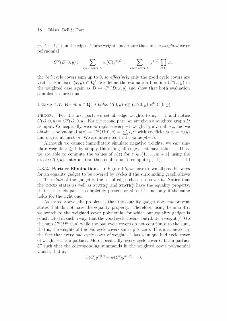
4.3.2. Partner Elimination. In Figure 4.5, we have drawn all possible waysfor an equality gadget to be covered by cycles if the surrounding graph allowsit. The state of the gadget is the set of edges chosen to cover it. Notice thatthe good states as well as state±
1 and state±2 have the equality property,
that is, the left path is completely present or absent if and only if the sameholds for the right one.
As stated above, the problem is that the equality gadget does not preventstates that do not have the equality property. Therefore, using Lemma 4.7,we switch to the weighted cover polynomial for which our equality gadget isconstructed in such a way, that the good cycle covers contribute a weight 6= 0 tothe sum Cw(Dα; 0, y) while the bad cycle covers do not contribute to the sum,that is, the weights of the bad cycle covers sum up to zero. This is achieved bythe fact that every bad cycle cover of weight +1 has a unique bad cycle coverof weight −1 as a partner. More specifically, every cycle cover C has a partnerC ′ such that the corresponding summands in the weighted cover polynomialvanish, that is,
w(C)yσ(C) + w(C ′)yσ(C′) = 0.
Complexity and Approximability of the Cover Polynomial 19
u
v
u′
v′
u
v
u′
v′
u
v
u′
v′
−1
good1 state+1 state−
1
u
v
u′
v′
u
v
u′
v′
u
v
u′
v′
−1
good2 state+2 state−
2
u
v
u′
v′
−1
u
v
u′
v′
u
v
u′
v′
−1
good3 state+3 state−
3
u
v
u′
v′
u
v
u′
v′
−1
state+4 state−
4
Figure 4.5: All possible states (=partial cycle covers) of the equality gadgetexcept that the states state±
3 and state±4 also have symmetric cases, which
we have not drawn. We call good1, good2, and good3 good states as theyhave no partners and satisfy the equality property. Note that the choice ofthe good states is arbitrary as long as the equality property is satisfied and allstate±
i have partners.
20 Blaser, Dell & Fouz
Note that not only the weights must be of different sign, but also the numbersof cycles must be equal! This is the crucial factor why we cannot simply adaptthe XOR-gadget of Valiant to form an equality gadget for the cover polynomial.The number of cycles contributed by his XOR-gadget varies a lot, and thus thesummands corresponding to the bad cycle covers do not cancel out. (If we plugin y = 1 to get the permanent, the condition on the cycles is not needed, andthe XOR-gadget works, of course.)
Now let us quickly summarize and prove the properties of the equalitygadget. We now call a cycle cover bad if an equality gadget is in a statestate±
i . The following lemma shows that there exists an involution on theset of bad cycle covers which switches the sign of the weights and leaves thenumber of cycles untouched.
Lemma 4.8. Every bad cycle cover C of Dα has a partner C ′ with the prop-erties
(i) C ′ is again bad, and its partner is C,
(ii) for the weights, it holds w(C ′) = −w(C), and
(iii) for the number of cycles, it holds σ(C ′) = σ(C).
Proof. We choose an arbitrary ordering on the equality gadgets of Dα. LetC be a bad cycle cover and g be its smallest gadget in state state±
i . We defineits partner C ′ to be the same cycle cover but with gadget g in state state∓
i
instead. Verifying the three properties proves the claim. �
It immediately follows that only the good cycle covers of Dα remain in Cw(Dα):
Cw(Dα; 0, y) =∑
cycle cover C,C is good
w(C)yσ(C).
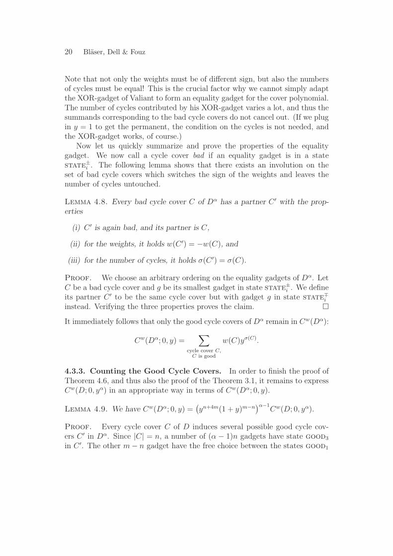
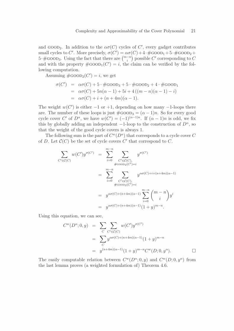
4.3.3. Counting the Good Cycle Covers. In order to finish the proof ofTheorem 4.6, and thus also the proof of the Theorem 3.1, it remains to expressCw(D; 0, yα) in an appropriate way in terms of Cw(Dα; 0, y).
Lemma 4.9. We have Cw(Dα; 0, y) =(
yn+4m(1 + y)m−n)α−1
Cw(D; 0, yα).
Proof. Every cycle cover C of D induces several possible good cycle cov-ers C ′ in Dα. Since |C| = n, a number of (α − 1)n gadgets have state good3
in C ′. The other m− n gadget have the free choice between the states good1
Complexity and Approximability of the Cover Polynomial 21
and good2. In addition to the ασ(C) cycles of C ′, every gadget contributessmall cycles to C ′. More precisely, σ(C ′) = ασ(C)+4 ·#good1 +5 ·#good2 +5 ·#good3. Using the fact that there are
(
m−n
i
)
possible C ′ corresponding to Cand with the property #good1(C
′) = i, the claim can be verified by the fol-lowing computation.
Assuming #good2(C′) = i, we get
σ(C ′) = ασ(C) + 5 · #good3 + 5 · #good2 + 4 · #good1
= ασ(C) + 5n(α − 1) + 5i + 4 ((m − n)(α − 1) − i)
= ασ(C) + i + (n + 4m)(α − 1).
The weight w(C ′) is either −1 or +1, depending on how many −1-loops thereare. The number of these loops is just #good3 = (α− 1)n. So for every goodcycle cover C ′ of Dα, we have w(C ′) = (−1)(α−1)n. If (α − 1)n is odd, we fixthis by globally adding an independent −1-loop to the construction of Dα, sothat the weight of the good cycle covers is always 1.
The following sum is the part of Cw(Dα) that corresponds to a cycle cover Cof D. Let C(C) be the set of cycle covers C ′ that correspond to C.
∑
C′∈C(C)
w(C ′)yσ(C′) =
m−n∑
i=0
∑
C′∈C(C),#good2(C′)=i
yσ(C′)
=m−n∑
i=0
∑
C′∈C(C),#good2(C′)=i
yασ(C)+i+(n+4m)(α−1)
= yασ(C)+(n+4m)(α−1)
m−n∑
i=0
(
m − n
i
)
yi
= yασ(C)+(n+4m)(α−1)(1 + y)m−n.
Using this equation, we can see,
Cw(Dα; 0, y) =∑
C
∑
C′∈C(C)
w(C ′)yσ(C′)
=∑
C
yασ(C)+(n+4m)(α−1)(1 + y)m−n
= y(n+4m)(α−1)(1 + y)m−nCw(D; 0, yα). �
The easily computable relation between Cw(Dα; 0, y) and Cw(D; 0, yα) fromthe last lemma proves (a weighted formulation of) Theorem 4.6.

22 Blaser, Dell & Fouz
Finally, the part of Theorem 3.1 concerned with the factorial cover polyno-mial follows, for −1 6= y 6= 0, from the reduction chain
C(0, 1) 4pT Cw(0, 1) 4p
T Cw(0, y) 4pT C(0, y) 4p
T C(x, y).
4.4. The Geometric Cover Polynomial. The geometric cover polynomialCgeo(D; x, y) introduced by D’Antona & Munarini (2000) is the geometric ver-sion of the cover polynomial, that is, the falling factorial xρ is replaced by theusual power xρ in (2.6).
Cgeo(D; x, y) :=∑
ρ,σ
cD(ρ, σ)xρyσ.
We denote by Dα-thick the α-thickening of a graph D in which every directededge is replaced by α directed (multi-)edges. This graph operation gives ahorizontal reduction for the geometric cover polynomial.
Lemma 4.10. For α ∈ N>0, it holds Cgeo(Dα-thick; x, y) = αnCgeo(D; x/α, y).
Proof. Let C be the set of all path-cycle covers of D. Every path-cycle coverPC ∈ C satisfies ρ(PC) = n − |PC| and gives rise to exactly α|PC| = αn−ρ(PC)
path-cycle covers of Dα-thick. Each of them has the same numbers of cycles andpaths as PC. Thus,
Cgeo(Dα-thick; x, y) =
∑
PC∈C
αn−ρ(PC)xρ(PC)yσ(C) = αnCgeo(D; x/α, y). �
An immediate corollary of the lemma above, together with interpolation, is thereduction Cgeo(x
′, y) 4pT Cgeo(x, y), for all x, x′, y ∈ Q with x 6= 0. Using these
horizontal reductions, we can prove a dichotomy theorem for the geometriccover polynomial.
Theorem 4.11. Let (x, y) ∈ Q2.If (x, y) 6∈
{
(0, 0), (0,−1)}
, then Cgeo(x, y) is #P-hard.Otherwise, Cgeo(x, y) is computable in polynomial time.
Proof. On the y-axis, geometric and factorial cover polynomial coincide,Cfac(D; 0, y) = Cgeo(D; 0, y). Thus, for x = 0, the result follows from thefactorial cover polynomial part of Theorem 3.1. For points with x 6= 0 andy 6= 0,−1, we use the horizontal reduction from above to reduce from they-axis to Cgeo(x, y).

Complexity and Approximability of the Cover Polynomial 23
For y = 0,−1, we again use thickenings as above to compute the polynomialCgeo(D; x, y) =
∑
ρ cρxρ with coefficients cρ =
∑
σ cD(ρ, σ)yσ. For y = 0, thecoefficient c1 = cD(1, 0) = #HamiltonianPaths(D) is #P-hard. For y = −1,note that three coefficients can be used to compute a hard point of the factorialcover polynomial: Cfac(D; 2,−1) = c0 + 2c1 + 2c2. �
5. Inapproximability of the Geometric Cover Polynomial
In this section, we study the approximability of Cgeo(x, y). In particular, weprove the following theorem.
Theorem 5.1. Let (x, y) ∈ Q2 with y 6= 1 and (x, y) /∈{
(0, 0), (0,−1)}
suchthat there is a digraph D with Cgeo(D; x, y) = 0.
For y > 0 or y ≤ 0 approximating Cgeo(x, y) is not possible within anypolynomial factor unless RP = NP or RFP = #P, respectively.
Both versions of the cover polynomial are self-reducible because the contraction-deletion identities (2.7) reduce the evaluation to smaller instances in polynomialtime. Hence, we know by Theorem 2.4 that Cgeo(x, y) either has an FPRAS oris inapproximable within any polynomial factor.
The proof proceeds as follows. First, we establish the inapproximability ofthe y-axis. In particular, we prove that an FPRAS for the positive or negativey-axis would entail RP = NP or RFP = #P, respectively. We make anexception at three points: Cgeo(0, 0) is trivially zero, Cgeo(1, 0) is the permanent,and Cgeo(−1, 0) basically is the determinant. Second, we give an approximationpreserving (horizontal) reduction from (0, y) to any point (x, y) for which thereexists a digraph D with Cgeo(D; x, y) = 0. Hence, we can carry over theinapproximability results of the y-axis to these points. Since Cgeo(0, 0) andCgeo(0,−1) are polynomial-time computable, we will separately establish theinapproximability of Cgeo(−1, 0) and Cgeo(−1,−1), and give an approximationpreserving reduction on these two lines. Unfortunately, this approach fails forthe factorial cover polynomial since the gadgets used in the reductions rely onthe product rule of the geometric cover polynomial that the factorial versionlacks in general.
We note that Cgeo(x, 1) can be approximated by an FPRAS for x ≥ 0. Forx = 0, this is due to the fact that the permanent Cgeo(0, 1) has an FPRAS,as recently discovered by Jerrum et al. (2004). For x > 0, Cgeo(x, 1) can beapproximation-preservingly reduced to the matching polynomial M(G; x), forwhich Jerrum & Sinclair (1997) gave an FPRAS in the case x > 0. Hence, weobtain the following lemma.
24 Blaser, Dell & Fouz
Lemma 5.2. There exists an FPRAS for Cgeo(x, 1) if x ≥ 0.
5.1. Inapproximability of the y-Axis. As we will see, the y-axis exhibitsdifferent levels of inapproximability. Whereas its positive part is inapprox-imable under the reasonable assumption RP 6= NP, it turns out that approx-imating its negative part is as hard as #P. We will therefore consider bothcases separately.
5.1.1. The Positive y-Axis. We consider the two cases y ∈ (0, 1) and y > 1separately.
Lemma 5.3. For y ∈ (0, 1), approximating Cgeo(0, y) is not possible within anypolynomial factor unless RP = NP.
Proof. Consider Cgeo(D; 0, y) =∑
σ cD(0, σ)yσ. Note that cD(0, 1) denotesthe number of Hamiltonian cycles in D. As is well known, it is NP-hard todecide whether cD(0, 1) 6= 0. Our goal is to amplify the contribution of thissummand to the whole sum such that an approximation algorithm for Cgeo(0, y)would allow us to decide whether D contains a Hamiltonian cycle.
We will now demonstrate the idea of the amplification. Similar to theconstruction for the #P-hardness proof, we would want to build a graph Dk
containing k copies of D that are connected in such a way that every cycle coverof Dk is (essentially) a cycle cover of D copied k times, and thus, has k timesas many cycles as the corresponding cycle cover of D. Assuming the existenceof such a ‘perfect cloning construction’, we get
PerfectCloning(D, k; 0, y) :=∑
σ
cD(0, σ)ykσ
= cD(0, 1)yk +∑
σ>1
cD(0, σ)ykσ
≤ yk(
cD(0, 1) + yk∑
σ>1
cD(0, σ))
[y ∈ (0, 1)]
≤ yk(
cD(0, 1) + yk2m)
. [#cycle covers ≤ 2m]
By choosing k ∈ O(m) such that yk2m < 12, we have
PerfectCloning(D, k; 0, y) < yk(
cD(0, 1) + 12
)
.
Now we can see that a cloning construction amplifies Hamiltonian cycles in thefollowing sense:
Complexity and Approximability of the Cover Polynomial 25
u
v
u′
v′
u
v
u′
v′
e e′
ℓ
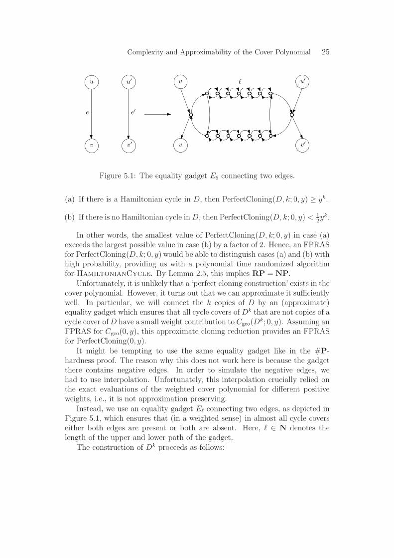
Figure 5.1: The equality gadget E6 connecting two edges.
(a) If there is a Hamiltonian cycle in D, then PerfectCloning(D, k; 0, y) ≥ yk.
(b) If there is no Hamiltonian cycle in D, then PerfectCloning(D, k; 0, y) < 12yk.
In other words, the smallest value of PerfectCloning(D, k; 0, y) in case (a)exceeds the largest possible value in case (b) by a factor of 2. Hence, an FPRASfor PerfectCloning(D, k; 0, y) would be able to distinguish cases (a) and (b) withhigh probability, providing us with a polynomial time randomized algorithmfor HamiltonianCycle. By Lemma 2.5, this implies RP = NP.
Unfortunately, it is unlikely that a ‘perfect cloning construction’ exists in thecover polynomial. However, it turns out that we can approximate it sufficientlywell. In particular, we will connect the k copies of D by an (approximate)equality gadget which ensures that all cycle covers of Dk that are not copies of acycle cover of D have a small weight contribution to Cgeo(D
k; 0, y). Assuming anFPRAS for Cgeo(0, y), this approximate cloning reduction provides an FPRASfor PerfectCloning(0, y).
It might be tempting to use the same equality gadget like in the #P-hardness proof. The reason why this does not work here is because the gadgetthere contains negative edges. In order to simulate the negative edges, wehad to use interpolation. Unfortunately, this interpolation crucially relied onthe exact evaluations of the weighted cover polynomial for different positiveweights, i.e., it is not approximation preserving.
Instead, we use an equality gadget Eℓ connecting two edges, as depicted inFigure 5.1, which ensures that (in a weighted sense) in almost all cycle coverseither both edges are present or both are absent. Here, ℓ ∈ N denotes thelength of the upper and lower path of the gadget.
The construction of Dk proceeds as follows:

26 Blaser, Dell & Fouz
1. Take k copies D1, . . . , Dk of D.
2. Let ei be the edge in Di corresponding to e in D. Connect all corre-sponding edges
{
e1, . . . , ek
}
by a cascade of equality gadgets Eℓ, for asufficiently (polynomially) large even ℓ, as shown in Figure 4.4.
Note that each edge of Di is split into at most three edges in step 2 and thatthe construction uses (k − 1)m equality gadgets.
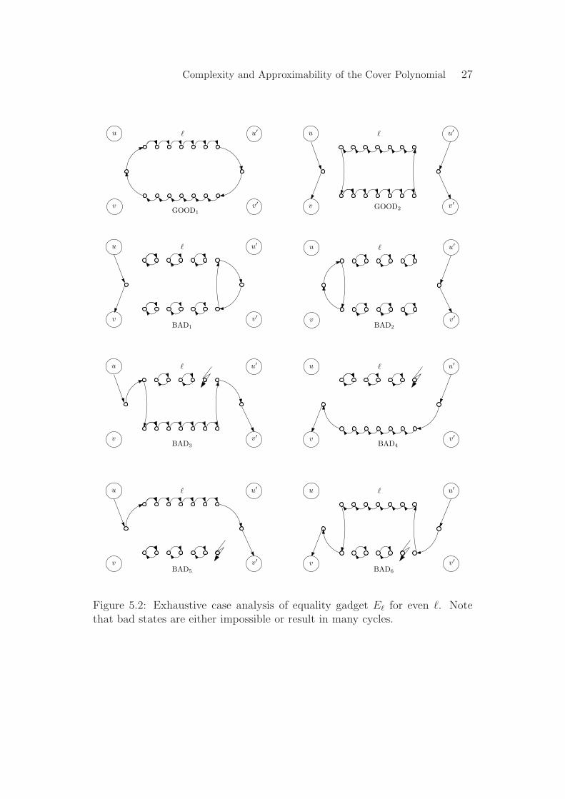
We now prove that the equality gadget indeed works sufficiently well tomake sure that a cycle cover of D1 carries over to all other Di in almost allcases (in a weighted sense). In Figure 5.2, the four possible situations of theequality gadget Eℓ are drawn for even ℓ, besides four impossible situations ofbad states. It is easy to see that, for each possible configuration of the outeredges, there is at most one possible way to complete it to a cycle cover on thegadget. Since each edge of Di is split into at most three edges, it follows thatthere are at most 23mk cycle covers of Dk.
The crucial point is that, while in the good states (both outer paths absentor both outer paths present) each gadget only adds a single cycle to the existingcycle cover, we get ℓ + 1 additional cycles in the bad states. So although theequality gadget cannot prevent the occurrence of a bad case completely, it willadd a factor of yℓ+1 to the weight of the corresponding cycle cover. We call cyclecovers of Dk bad if at least one gadget is in a bad state, and good otherwise.
Since the good cycle covers simulate perfect cloning, we get
Cgeo(Dk; 0, y) =
∑
bad cycle cover C
yσ(C) +∑
good cycle cover C
yσ(C)
≤ 23mkyℓ+1 + y(k−1)m · PerfectCloning(D, k; 0, y)
<(
1 +1
4
)
y(k−1)m · PerfectCloning(D, k; 0, y),
by choosing ℓ ∈ O(k2m2) sufficiently large, such that 23mkyℓ+1 < 14ykm. If D
has at least one cycle cover, then PerfectCloning(D, k; 0, y) ≥ ym and thesecond inequality above is true (if not, we just return 0). On the otherhand, Cgeo(D
k; 0, y) ≥ y(k−1)mPerfectCloning(D, k; 0, y) since y > 0. Thus,an FPRAS for Cgeo(0, y) would entail an FPRAS for PerfectCloning(0, y). Butthis implies RP = NP as we have seen before. This finishes the case y ∈ (0, 1).
�
Remark 5.4. Note that the ‘approximate cloning reduction’ also proves thatthere cannot be a randomized polynomial time algorithm that approximates
Complexity and Approximability of the Cover Polynomial 27
u
v
u′
v′
ℓ
u
v
u′
v′
ℓ u
v
u′
v′
ℓ
u
v
u′
v′
ℓ
u
v
u′
v′
ℓ u
v
u′
v′
ℓ
u
v
u′
v′
ℓ u
v
u′
v′
ℓ
BAD1 BAD2
BAD3 BAD4
BAD5 BAD6
GOOD1
GOOD2
Figure 5.2: Exhaustive case analysis of equality gadget Eℓ for even ℓ. Notethat bad states are either impossible or result in many cycles.
28 Blaser, Dell & Fouz
u
v
u′
v′
u
v
u′
v′
e e′
ℓ
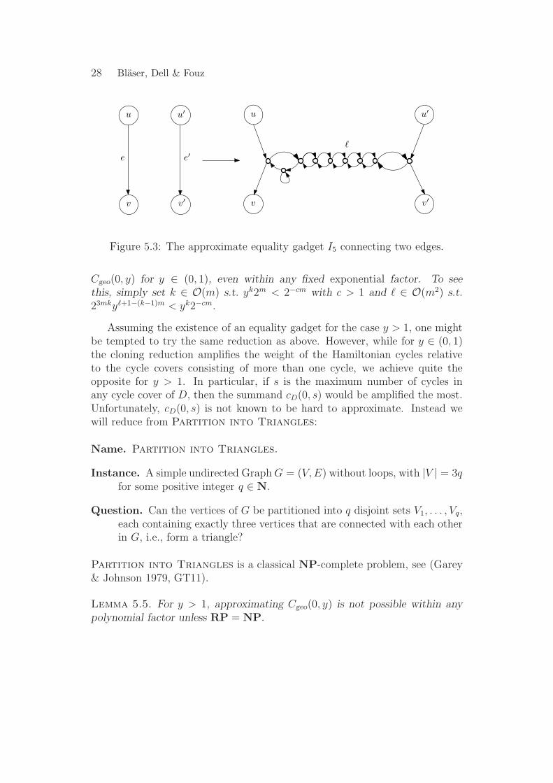
Figure 5.3: The approximate equality gadget I5 connecting two edges.
Cgeo(0, y) for y ∈ (0, 1), even within any fixed exponential factor. To seethis, simply set k ∈ O(m) s.t. yk2m < 2−cm with c > 1 and ℓ ∈ O(m2) s.t.23mkyℓ+1−(k−1)m < yk2−cm.
Assuming the existence of an equality gadget for the case y > 1, one mightbe tempted to try the same reduction as above. However, while for y ∈ (0, 1)the cloning reduction amplifies the weight of the Hamiltonian cycles relativeto the cycle covers consisting of more than one cycle, we achieve quite theopposite for y > 1. In particular, if s is the maximum number of cycles inany cycle cover of D, then the summand cD(0, s) would be amplified the most.Unfortunately, cD(0, s) is not known to be hard to approximate. Instead wewill reduce from Partition into Triangles:
Name. Partition into Triangles.
Instance. A simple undirected Graph G = (V, E) without loops, with |V | = 3qfor some positive integer q ∈ N.
Question. Can the vertices of G be partitioned into q disjoint sets V1, . . . , Vq,each containing exactly three vertices that are connected with each otherin G, i.e., form a triangle?
Partition into Triangles is a classical NP-complete problem, see (Garey& Johnson 1979, GT11).
Lemma 5.5. For y > 1, approximating Cgeo(0, y) is not possible within anypolynomial factor unless RP = NP.
Complexity and Approximability of the Cover Polynomial 29
u′
v′
u
v
u′
v′
e e′
u
v
Iq
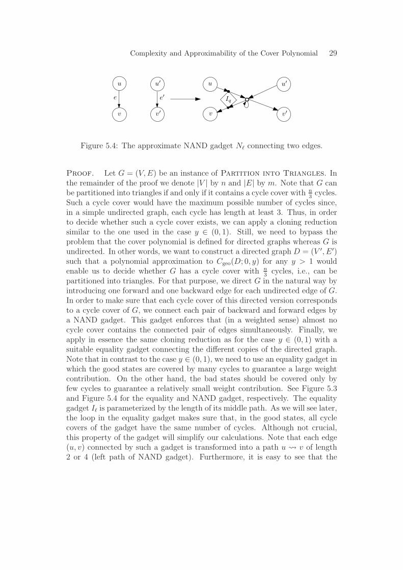
Figure 5.4: The approximate NAND gadget Nℓ connecting two edges.
Proof. Let G = (V, E) be an instance of Partition into Triangles. Inthe remainder of the proof we denote |V | by n and |E| by m. Note that G canbe partitioned into triangles if and only if it contains a cycle cover with n
3cycles.
Such a cycle cover would have the maximum possible number of cycles since,in a simple undirected graph, each cycle has length at least 3. Thus, in orderto decide whether such a cycle cover exists, we can apply a cloning reductionsimilar to the one used in the case y ∈ (0, 1). Still, we need to bypass theproblem that the cover polynomial is defined for directed graphs whereas G isundirected. In other words, we want to construct a directed graph D = (V ′, E ′)such that a polynomial approximation to Cgeo(D; 0, y) for any y > 1 wouldenable us to decide whether G has a cycle cover with n
3cycles, i.e., can be
partitioned into triangles. For that purpose, we direct G in the natural way byintroducing one forward and one backward edge for each undirected edge of G.In order to make sure that each cycle cover of this directed version correspondsto a cycle cover of G, we connect each pair of backward and forward edges bya NAND gadget. This gadget enforces that (in a weighted sense) almost nocycle cover contains the connected pair of edges simultaneously. Finally, weapply in essence the same cloning reduction as for the case y ∈ (0, 1) with asuitable equality gadget connecting the different copies of the directed graph.Note that in contrast to the case y ∈ (0, 1), we need to use an equality gadget inwhich the good states are covered by many cycles to guarantee a large weightcontribution. On the other hand, the bad states should be covered only byfew cycles to guarantee a relatively small weight contribution. See Figure 5.3and Figure 5.4 for the equality and NAND gadget, respectively. The equalitygadget Iℓ is parameterized by the length of its middle path. As we will see later,the loop in the equality gadget makes sure that, in the good states, all cyclecovers of the gadget have the same number of cycles. Although not crucial,this property of the gadget will simplify our calculations. Note that each edge(u, v) connected by such a gadget is transformed into a path u v of length2 or 4 (left path of NAND gadget). Furthermore, it is easy to see that the
30 Blaser, Dell & Fouz
cycle cover of the gadgets is uniquely determined by the presence or absence oftheir outer paths, see Figure 5.5 and Figure 5.6. Hence, it is sufficient for thecloning reduction to connect the corresponding outer paths of each copy of Dby equality gadgets. Formally, the construction of Dk proceeds as follows:
1. Start with D = (V ′, E ′) where V ′ = V and E ′ =⋃
{u,v}∈E(u, v) ∪ (v, u)
2. Connect each pair {(u, v), (v, u)} ⊆ E ′ by the NAND gadget Nℓ for suf-ficiently (polynomially) large odd ℓ ∈ N.
3. Construct Dk as follows:
(a) Take k copies D1, . . . , Dk of D for a sufficiently (polynomially) largek ∈ N.
(b) Let ei be an edge in Di corresponding to an edge e on an outer pathof a gadget in D. Connect all corresponding edges {e1, . . . , ek} by acascade of equality gadgets Iℓ for a sufficiently (polynomially) largeodd ℓ, see Figure 4.4.
Each undirected edge {u, v} of G is transformed into two directed edges(u, v) and (v, u) in step 1, that are split into at most four outer edges in step2, which in turn are copied k times where each copy is split into at most threeedges in step 3. In total, Dk has at most 24km outer edges. Since the cyclecover of every gadget is uniquely determined by the outer edges of its gadgets,it follows that Dk has at most 224km cycle covers.
We will now prove that both types of used gadgets work sufficiently well forour purposes. It is easy to see that the NAND gadget works as desired underthe assumption that the equality gadget does so. In Figure 5.6, all states thatare compatible with good states of the equality gadget are shown. In particular,note that only one of the two paths u v and u′ v′ can be present in acycle cover since they share a common vertex in the middle. Moreover theequality gadget Iℓ enforces that cycle covers in which the invalid pathes u v′
or u′ v are present contribute only a relatively small weight. Note that theNAND gadget provides one additional cycle if its outer paths are absent.
As for the proposed equality gadget, we prove that bad states of cycle coverswhere only one of the two connected edges is present have a relatively smallweight. In Figure 5.5 all possible states of Iℓ are illustrated for odd ℓ, besidestwo impossible bad states. Note that in the good states (both edges present orabsent), the equality gadget Iℓ provides ℓ+3
2additional cycles to the cycle cover.
On the other hand, at most one additional cycle occurs in the bad states.

Complexity and Approximability of the Cover Polynomial 31
u
v
u′
v′
ℓ
u
v
u′
v′
ℓ
u
v
u′
v′
ℓ
u
v
u′
v′
ℓ
u
v
u′
v′
ℓ
u
v
u′
v′
ℓ
GOOD1 GOOD2
BAD1 BAD2
BAD3 BAD4
Figure 5.5: Exhaustive case analysis of equality gadget Iℓ for odd ℓ. Note thatgood states incur many cycles, wheras bad states are either impossible or haveat most one cycle.
u′
v′
u
v
Iq
u′
v′
u
v
Iq
u′
v′
u
v
Iq
Figure 5.6: Case analysis of NAND gadget Nℓ for odd ℓ. Bad states resultingfrom bad states of the equality gadget are omitted.
32 Blaser, Dell & Fouz
As before, we call cycle covers of Dk good if all gadgets are in a good stateand bad otherwise. Hence, good cycle covers of Dk (essentially) consist of kcopies of cycle covers of D where each cycle has length at least 3.
First, we note that Dk contains k ·m Nℓ gadgets and (k−1) ·2m additionalIℓ gadgets. Since each Nℓ gadget is made up of one Iℓ gadgets, we have in total3km− 2m Iℓ gadgets. Thus, on the one hand, a good cycle cover gets a weightfactor of exactly y(3km−2m) ℓ+3
2 from its equality gadgets. Furthermore, it getsa weight factor of yk(m−n) from its NAND gadgets since there are m − n pairsof connected edges that are absent in a cycle cover. On the other hand, a badcycle cover gets at most a weight factor of y(3km−2m−1) ℓ+3
2+1 from its equality
gadgets since, by definition, at least one of its equality gadgets is in a bad state.Apart from that, it gets at most a weight factor of ykm from its NAND gadgets.Besides the cycles from the gadgets, a bad cycle cover can have at most 1
2kn
cycles, since we assumed that G has no loops.Following the now familiar path,
Cgeo(Dk; 0, y) =
∑
bad cycle cover C
yσ(C) +∑
good cycle cover C
yσ(C)
≤ 224kmy(3km−2m−1) ℓ+3
2+1ykmy
1
2kn
[
# of cycle covers
+ y(3km−2m) ℓ+3
2 yk(m−n)∑
σ
cD(0, σ)ykσ is ≤ 224km]
= y(3km−2m) ℓ+3
2+k(m−n)
(
224kmy1
2(3kn−ℓ−1)
[
good cycle cover
+ cD(0, n3)y
1
3kn +
∑
σ< n
3
cD(0, σ)ykσ)
has ≤ n3
cycles]
≤ y(3km−2m) ℓ+3
2+k(m−n)
(
224kmy1
2(3kn−ℓ−1)
[
# of cycle covers
+ cD(0, n3)y
1
3kn + 22myk(n
3−1)
)
of D is ≤ 22m]
= y(3km−2m) ℓ+3
2+k(m−n)+ 1
3kn
(
224kmy1
2( 7
3kn−ℓ−1)
+ cD(0, n3) + 22my−k
)
.
By setting k ∈ O(m) s.t. 22my−k < 14
and ℓ ∈ O(m2) s.t. 224kmy1
2( 7
3kn−ℓ−1) < 1
4,
we have
Cgeo(Dk; 0, y) < y(3km−2m) ℓ+3
2+k(m−n)+ 1
3kn
(
12
+ cD(0, n3))
.
We consider the two complementary situations:
(a) There exists a partition of G into triangles. Then cD(0, n3) ≥ 1 and
Cgeo(Dk; 0, y) ≥ y(3km−2m) ℓ+3
2+k(m−n)+ 1
3kn.
Complexity and Approximability of the Cover Polynomial 33
(b) There exists no partition of G into triangles. Then cD(0, n3) = 0 and
Cgeo(Dk; 0, y) < 1
2y(3km−2m) ℓ+3
2+k(m−n)+ 1
3kn.
By the same argument as in the case y ∈ (0, 1), the existence of an FPRASfor Cgeo(0, y) for y > 1 would entail RP = NP. �
5.1.2. The Negative y-Axis. We can easily adapt the above proof for thecorresponding negative cases. In particular, we can use the same gadgets forour reductions. We refrain from doing so since, for y < 0, we will prove the evenstronger statement that approximating Cgeo(0, y) is as hard as #P. Assumingthat #P is a much bigger class than RFP, this is a very different kind ofinapproximability. As noted before (see Corollary 2.2), every problem in #PQ
has a randomized polynomial approximation scheme using an oracle for an NPpredicate. Based on this fact, our result implies that, for negative y, Cgeo(0, y)is not in #PQ, under a reasonable complexity assumption.
Theorem 5.6. For y ∈ Q− \ {−1}, approximating Cgeo(0, y) is not possiblewithin any polynomial factor unless RFP = #P.
Proof (sketch). Assuming the existence of an FPRAS for Cgeo(0, y), we willshow how to compute the exact value of Cgeo(0, y) which is known to be #P-hard. This will establish Theorem 5.6.
The proof proceeds as follows. For two given directed graphs D1, D2, wewill show how to construct a digraph Dℓ
1,2 such that, for some polynomiallylarge ℓ ∈ N,
Cgeo(Dℓ1,2; 0, y) ≈ Cgeo(D1; 0, y) + Cgeo(D2; 0, y).
Given such a construction, we will show how, for z ∈ Q, we can build adigraph Dz such that Cgeo(Dz; 0, y) ≈ z. Both these building blocks will enableus to perform a binary search over a precomputed interval of possible values ofCgeo(D; 0, y) for any directed graph D. �
Let us now turn to our first goal. We construct Dℓ1,2 by first taking the
disjoint union of D1 and D2. We want to connect both subgraphs such thatideally the cycle covers of Dℓ
1,2 are in one-to-one correspondence with the cyclecovers of D1 and D2. For that purpose, we connect both subgraphs in such away that (in a weighted sense) almost all cycle covers of Dℓ
1,2 consist of cyclecovers of D1 and one designated cycle cover on D2, or vice versa, consist of cyclecovers of D2 and one designated cycle cover on D1. Thus, the cycle covers of
34 Blaser, Dell & Fouz
u
v
u′
v′
e e′
u
v
=ℓ
u′
v′
=ℓ
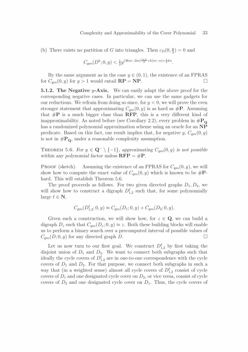
Figure 5.7: The implies gadget Impℓ.
Dℓ1,2 can be seen as disjoint unions of the cycle covers of D1 and D2. It follows
that Cgeo(Dℓ1,2; 0, y) is (almost) the sum of Cgeo(D1; 0, y) and Cgeo(D2; 0, y).
The disjoint union is achieved by adding a Hamiltonian cycle H1 to D1 andconnecting its edges by equality gadgets, and adding a Hamiltonian cycle H2
to D2 and also connecting its edges by equality edges. Finally, each originaledge of D1 gets connected with an arbitrary edge e0 of the new Hamiltoniancycle H2 by an ‘implies gadget’. Such a gadget enforces that, (in a weightedsense) in almost all cycle covers, whenever an edge in D1 is taken (other thanfrom H1), e0 is also taken, and in turn, because of the equality gadgets, H2 isused to cover D2. Vice versa, the construction makes sure that, (in a weightedsense) in almost all cycle covers, if an edge in D2 is taken (other than fromH2), no edge in H2 can be taken simultaneously and thus D1 must be coveredby H1. As equality gadgets, we use the same gadgets as in the previous proof,Eℓ and Iℓ, for the cases y ∈ (−1, 0) and y < −1, respectively. Summarizing theconstruction, we have,
1. Start with Dℓ1,2 = D1 ⊎ D2 to be the disjoint union of D1 and D2. By
a slight abuse of notation, we will now denote by D1 and D2 the corre-sponding subgraphs of Dℓ
1,2.
2. Add two arbitrary Hamiltonian cycles H1 and H2 to D1 and D2, respec-tively, consisting of newly introduced edges. Note that this might resultin multiple edges.
3. Connect every pair of consecutive edges in H1 and H2 by equality gadgetsEℓ (resp. Iℓ), see Figure 4.4.
4. Connect each edge in D1 but not in H1 with a designated edge of H2 byan implies gadget Impℓ.
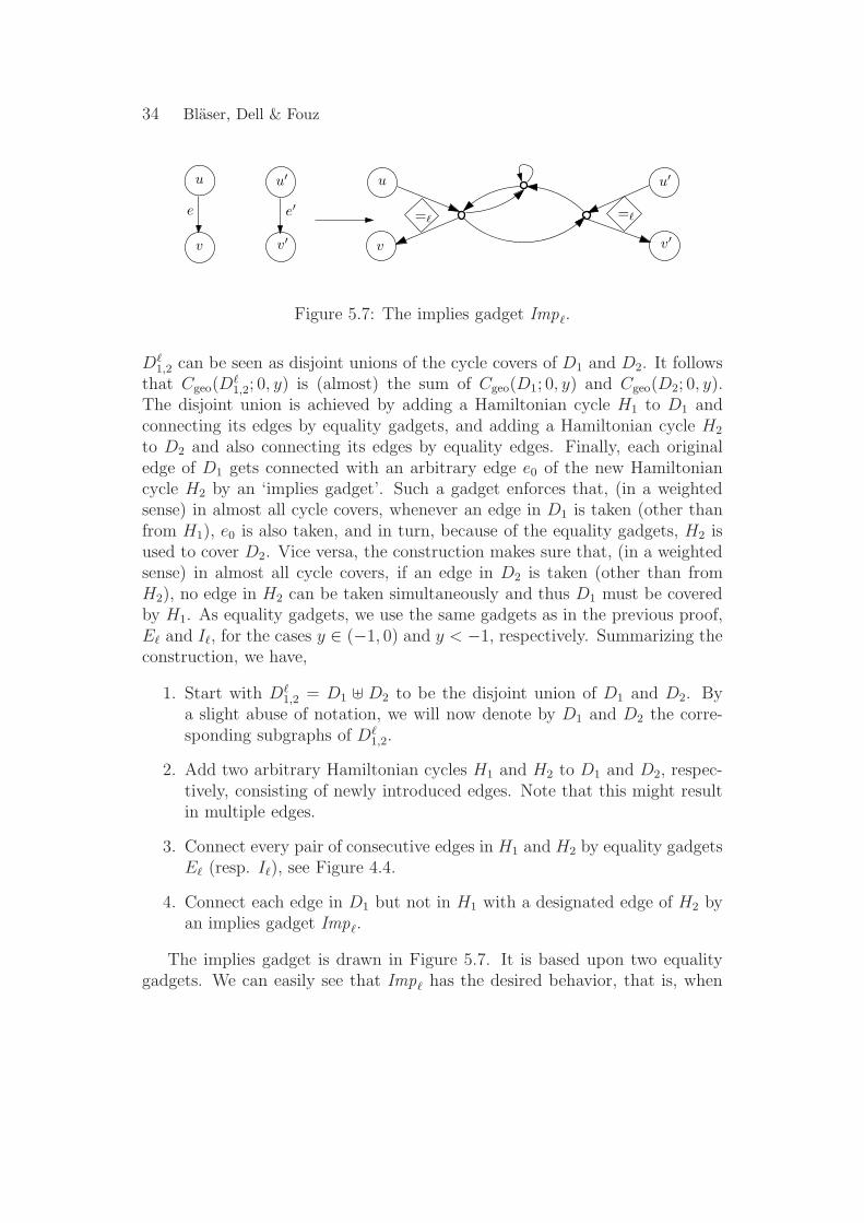
The implies gadget is drawn in Figure 5.7. It is based upon two equalitygadgets. We can easily see that Impℓ has the desired behavior, that is, when
Complexity and Approximability of the Cover Polynomial 35
u
v
=ℓ
u′
v′
=ℓ
u
v
=ℓ
u′
v′
=ℓ
u
v
=ℓ
u′
v′
=ℓ
Figure 5.8: Case analysis of approximate implies gadget Impℓ. Bad statesresulting from bad states of equality gadgets are omitted.
its left path u v is present in a cycle cover, then the right path u′ v′
does also have to be present (apart from the negligible bad states due to badstates of the equality gadgets), see Figure 5.8. Notice that all good states ofthe gadget add exactly one additional cycle to the corresponding cycle cover.
The following lemma assures that our construction works sufficiently well.
Lemma 5.7. Let D1, D2 be two digraphs, y ∈ Q, and r ∈ N an error param-eter. There exists k, ℓ ≤ poly(|D1| , |D2| , r) such that, for Dℓ
1,2 as constructedabove, it holds that
Cgeo(Dℓ1,2; 0, y) = yk
(
Cgeo(D1; 0, y) + Cgeo(D2; 0, y) + ǫ)
,
where |ǫ| < 2−r. Moreover, k and ℓ are computable in polynomial time.
Proof. Let ℓ ∈ N be a positive integer that will be specified later. Letn1 := n(D1), n2 := n(D2), m1 := m(D1), m2 := m(D2). First note that ourconstruction uses n1 equality gadgets for H1, n2 equality gadgets for H2 and2m1 equality gadgets for the m1 implies gadgets. Furthermore, every originaledge of D1 and H1 is split into at most four and three edges in Dℓ
1,2, respectively.Likewise, every original edge of H2 is split into into at most three edges exceptfor the designated edge of H2 which is split into 4m1 +2 edges. Since the cyclecover of every gadget is uniquely determined by its outer edges, we thus have
36 Blaser, Dell & Fouz
in total at most 24(2m1+n1+n2)+2 cycle covers of Dℓ1,2. We will now consider the
two cases, y ∈ (−1, 0) and y < −1, separately. In each case, we determine theweight contribution of the good cycle covers of Dℓ
1,2, and bound the absoluteweight contribution of the bad cycle covers of Dℓ
1,2.
Case y ∈ (−1, 0): In the good cycle covers, defined as before, the weightcontribution of the equality gadgets Eℓ (with even ℓ) is yn1+n2+2m1 , since eachequality gadget adds one cycle. Besides, each implies gadget also adds onecycle, incurring a factor of ym1. Finally, each good cycle cover of Dℓ
1,2 is a cyclecover of D1 or D2 with an additional Hamiltonian cycle on the other subgraph,respectively. In other words, there is a bijection between the cycle covers ofDℓ
1,2 and the union of the cycle covers of D1 and D2 which almost preserves thenumber of cycles. Hence, we get,
∑
goodcycle cover C
yσ(C) = yn1+n2+2m1 · ym1 ·(
yCgeo(D1; 0, y) + yCgeo(D2; 0, y))
= yn1+n2+3m1+1 ·(
Cgeo(D1; 0, y) + Cgeo(D2; 0, y))
.
In the bad cycle covers, at least one equality gadget is in a bad case, addingℓ + 1 cycles. It follows,
∣
∣
∣
∣
∑
badcycle cover C
yσ(C)
∣
∣
∣
∣
≤∣
∣yn1+n2+2m1−1 · yℓ+1∣
∣ · 24(2m1+n1+n2)+2
=∣
∣yn1+n2+3m1+1 · yℓ−m1−1∣
∣ · 24(2m1+n1+n2)+2.
In total, we get
Cgeo(Dℓ1,2; 0, y) =
∑
goodcycle cover C
yσ(C) +∑
badcycle cover C
yσ(C)
= yn1+n2+3m1+1 ·(
Cgeo(D1; 0, y) + Cgeo(D2; 0, y) + ǫ)
,
where |ǫ| ≤ |y|ℓ−m1−1 · 24(2m1+n1+n2)+2.
It is now easy to choose an even ℓ ∈ O(m1 +n1 +n2 +r) such that |ǫ| < 2−r.
Complexity and Approximability of the Cover Polynomial 37
Case y < −1: Noting that each equality gadget Iℓ adds ℓ+32
cycles in thegood cases (for odd ℓ), we get for the good cycle covers by the same line ofreasoning as in the previous case,
∑
goodcycle cover C
yσ(C) = y(n1+n2+2m1) ℓ+3
2 · ym1 · (yCgeo(D1; 0, y) + yCgeo(D2; 0, y))
= y(n1+n2+2m1) ℓ+3
2+m1+1 ·
(
Cgeo(D1; 0, y) + Cgeo(D2; 0, y))
.
In the bad cycle covers, at least one equality gadget is in a bad case, addingat most one cycle. Apart from that, each implies gadget adds at most onecycle. It follows,
∣
∣
∣
∣
∑
badcycle cover C
yσ(C)
∣
∣
∣
∣
≤∣
∣
∣y(n1+n2+2m1−1) ℓ+3
2 · y · ym1
∣
∣
∣· 24(2m1+n1+n2)+2
=∣
∣
∣y(n1+n2+2m1) ℓ+3
2+m1+1 · y− ℓ+3
2
∣
∣
∣· 24(2m1+n1+n2)+2.
In total, we have
Cgeo(Dℓ1,2; 0, y) =
∑
goodcycle cover C
yσ(C) +∑
badcycle cover C
yσ(C)
= y(n1+n2+2m1) ℓ+3
2+m1+1 ·
(
Cgeo(D1; 0, y) + Cgeo(D2; 0, y) + ǫ)
,
where |ǫ| ≤ |y|−ℓ+3
2 24(2m1+n1+n2)+2.Again, for some odd ℓ ∈ O(m1 + n1 + n2 + r), we have |ǫ| < 2−r. �
In the following, we denote by (D1 + D2)(r) the graph Dℓ1,2 with error
parameter r, as constructed above.We will now turn to our second building block of the proof of Theorem 5.6.
Our goal is to construct a directed graph Dz such that Cgeo(Dz; 0, y) ≈ z, wherez ∈ Q.
In case y is integer and z a non-integer value, we cannot hope to build adigraph Dz with Cgeo(Dz, 0, y) ≈ z. Instead, we will relax our original goal andshow how to construct a digraph Dz such that Cgeo(Dz; 0, y) = yc · z with cbeing an easily computable value. This relaxation is also necessary for a genericconstruction of Dz for non-integer y.
38 Blaser, Dell & Fouz
2 2
2 2 2
2 2 2 2
2 2 2 2 2 2
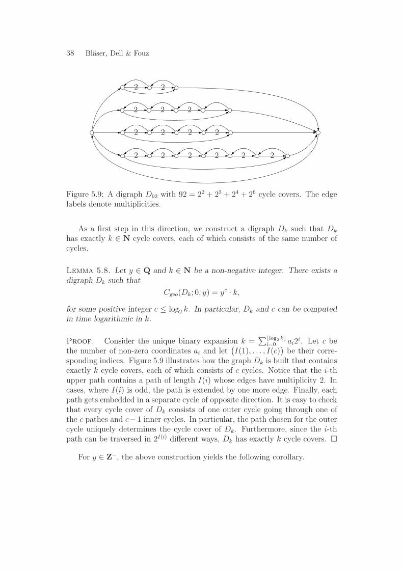
Figure 5.9: A digraph D92 with 92 = 22 + 23 + 24 + 26 cycle covers. The edgelabels denote multiplicities.
As a first step in this direction, we construct a digraph Dk such that Dk
has exactly k ∈ N cycle covers, each of which consists of the same number ofcycles.
Lemma 5.8. Let y ∈ Q and k ∈ N be a non-negative integer. There exists adigraph Dk such that
Cgeo(Dk; 0, y) = yc · k,
for some positive integer c ≤ log2 k. In particular, Dk and c can be computedin time logarithmic in k.
Proof. Consider the unique binary expansion k =∑⌊log2 k⌋
i=0 ai2i. Let c be
the number of non-zero coordinates ai and let(
I(1), . . . , I(c))
be their corre-sponding indices. Figure 5.9 illustrates how the graph Dk is built that containsexactly k cycle covers, each of which consists of c cycles. Notice that the i-thupper path contains a path of length I(i) whose edges have multiplicity 2. Incases, where I(i) is odd, the path is extended by one more edge. Finally, eachpath gets embedded in a separate cycle of opposite direction. It is easy to checkthat every cycle cover of Dk consists of one outer cycle going through one ofthe c pathes and c−1 inner cycles. In particular, the path chosen for the outercycle uniquely determines the cycle cover of Dk. Furthermore, since the i-thpath can be traversed in 2I(i) different ways, Dk has exactly k cycle covers. �
For y ∈ Z−, the above construction yields the following corollary.
Complexity and Approximability of the Cover Polynomial 39
Corollary 5.9. Let y ∈ Z− and z ∈ Z. There exists a digraph Dz, such that
Cgeo(Dz; 0, y) = yc · z,
for some positive integer c ∈ O(log |z|). In particular, Dz and c can be com-puted in time logarithmic in |z|.
Proof. If z ≥ 0, the claim directly follows from Lemma 5.8. Otherwise,apply Lemma 5.8 to get a graph Dyz such that Cgeo(Dyz; 0, y) = yc ·yz = yc+1 ·z.
�
For y ∈ Q− \ Z, we can extend the above construction to any z ∈ Q.
Lemma 5.10. Let y ∈ Q− \ Z, z ∈ Q be a rational value, and ℓ ∈ N be anerror parameter. There exists a digraph Dz, such that
Cgeo(Dz; 0, y) = yc(z + ǫ),
where c ≤ O(ℓ + log |z|) and 2−ℓ > ǫ ≥ 0. In particular, Dℓz can be build in
time polynomial in ℓ and log z.
Proof.
Again, we distinguish the cases y ∈ (−1, 0) and y < −1.
Case y ∈ (−1, 0): Assume for the moment that z ≥ 0. Our goal is toconstruct a digraph Dz such that Cgeo(Dz; 0, y) = ycyk · ⌈z ·y−k⌉, where c ∈ Z+,and k ∈ N is an even integer to be specified later. Applying Lemma 5.8, we firstconstruct a graph Dz with exactly ⌈z · y−k⌉ cycle covers. Let c ∈ O(k + log z)be the number of cycles of each of these cycle covers. Then, we add k disjointloops to Dz. Thus, we have Cgeo(Dz; 0, y) = ycyk · ⌈z · y−k⌉. By choosingk ∈ O(ℓ) such that yk < 2−ℓ, the claim follows.
If z < 0, we basically use the same construction, but choose k to be oddand build Dz such that it has ⌊z · y−k⌋ cycle covers.
Case y < −1: We use a similar construction as in case y ∈ (−1, 0). For thatpurpose, we construct a generic digraph Dr such that Cgeo(Dr; 0, y) ∈ (−1, 0).This graph Dr will take the role of the independent loops used in the previouscase.
Let y ∈ (−i,−i + 1) for some i ∈ Z+. Clearly, we have y + i ∈ (−1, 0).Unfortunately, there exists no digraph whose cover polynomial is y + i. Inparticular, every cover polynomial has an absolute term of zero. We can fix
40 Blaser, Dell & Fouz
a1
a2
a3
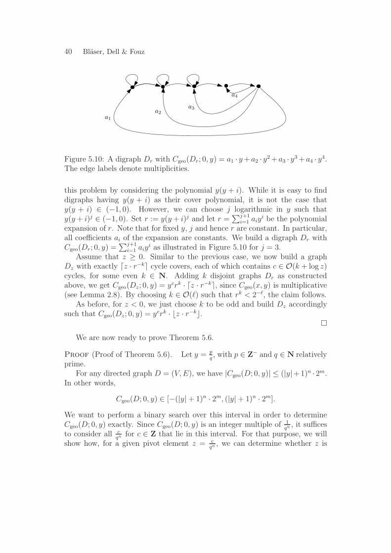
a4
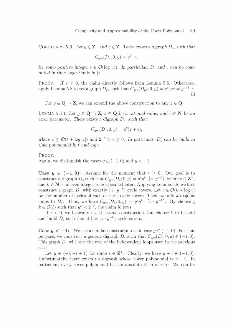
Figure 5.10: A digraph Dr with Cgeo(Dr; 0, y) = a1 · y + a2 · y2 + a3 · y
3 + a4 · y4.
The edge labels denote multiplicities.
this problem by considering the polynomial y(y + i). While it is easy to finddigraphs having y(y + i) as their cover polynomial, it is not the case thaty(y + i) ∈ (−1, 0). However, we can choose j logarithmic in y such thaty(y + i)j ∈ (−1, 0). Set r := y(y + i)j and let r =
∑j+1i=1 aiy
i be the polynomialexpansion of r. Note that for fixed y, j and hence r are constant. In particular,all coefficients ai of the expansion are constants. We build a digraph Dr withCgeo(Dr; 0, y) =
∑j+1i=1 aiy
i as illustrated in Figure 5.10 for j = 3.Assume that z ≥ 0. Similar to the previous case, we now build a graph
Dz with exactly ⌈z · r−k⌉ cycle covers, each of which contains c ∈ O(k + log z)cycles, for some even k ∈ N. Adding k disjoint graphs Dr as constructedabove, we get Cgeo(Dz; 0, y) = ycrk · ⌈z · r−k⌉, since Cgeo(x, y) is multiplicative(see Lemma 2.8). By choosing k ∈ O(ℓ) such that rk < 2−ℓ, the claim follows.
As before, for z < 0, we just choose k to be odd and build Dz accordinglysuch that Cgeo(Dz; 0, y) = ycrk · ⌊z · r−k⌋.
�
We are now ready to prove Theorem 5.6.
Proof (Proof of Theorem 5.6). Let y = p
q, with p ∈ Z− and q ∈ N relatively
prime.For any directed graph D = (V, E), we have |Cgeo(D; 0, y)| ≤ (|y|+1)n · 2m.
In other words,
Cgeo(D; 0, y) ∈ [−(|y| + 1)n · 2m, (|y| + 1)n · 2m].
We want to perform a binary search over this interval in order to determineCgeo(D; 0, y) exactly. Since Cgeo(D; 0, y) is an integer multiple of 1
qn , it sufficesto consider all c
qn for c ∈ Z that lie in this interval. For that purpose, we willshow how, for a given pivot element z = c
qn , we can determine whether z is
Complexity and Approximability of the Cover Polynomial 41
less, equal, or greater than Cgeo(D; 0, y). If z = 0, this distinction is equivalentto determine the sign of Cgeo(D; 0, y) which we can easily do having an FPRASat hand. Otherwise, let D−z be a graph as constructed in Corollary 5.9 orLemma 5.10 (depending on whether y is integer or non-integer, respectively),such that
(5.11) Cgeo(D−z; 0, y) = yc(−z + ǫ),
where c ∈ N is a polynomially computable integer and
(5.12) 0 ≤ ǫ ≤ 14q−n.
If y is integer we have ǫ = 0 by Corollary 5.9. If y is not integer, the lastinequality holds by Lemma 5.10 for ℓ ∈ O(n) such that 2−ℓ < 1
4q−n. In any
case, we have c ∈ O(ℓ + log z) = O(m + n).Let D′ be a copy of D with c additional independent disjoint loops. Thus,
(5.13) Cgeo(D′; 0, y) = ycCgeo(D; 0, y).
W.l.o.g. assume that c is even. Otherwise, we add one more independent loopto D−z and D′, respectively.
We consider the ‘sum’ of D′ and D−z with error parameter r ∈ O(m + n)such that
(5.14) 2−r < 14ycq−n.
We have,
Cgeo
(
(D′ + D−z)(r); 0, y)
= yk(
Cgeo(D′; 0, y)
+ Cgeo(D−z; 0, y) + ǫ′)
by Lemma 5.7
= yk(
ycCgeo(D; 0, y)
+ yc(−z + ǫ) + ǫ′)
by (5.13) and (5.11)
for some polynomially computable k ∈ N and by (5.14),
|ǫ′| < 14ycq−n.(5.15)
Equivalently,
(5.16) y−k Cgeo((D′ + D−z)(r); 0, y) = yc
(
Cgeo(D; 0, y)− z + ǫ)
+ ǫ′.
Now consider the three cases:
42 Blaser, Dell & Fouz
Case z ≥ Cgeo(D; 0, y) + q−n:
y−k Cgeo
(
(D′ + D−z)(r); 0, y)
≤ yc(−q−n + ǫ) + ǫ′ by (5.16)
< yc(−34q−n) + 1
4ycq−n by (5.12) and (5.15)
= −12ycq−n.
Case z ≤ Cgeo(D; 0, y) − q−n:
y−k Cgeo
(
(D′ + D−z)(r); 0, y)
≥ yc(q−n + ǫ) + ǫ′ by (5.16)
≥ ycq−n − 14ycq−n by (5.12) and (5.15)
= 34ycq−n.
Case z = Cgeo(D; 0, y):
y−k Cgeo
(
(D′ + D−z)(r); 0, y)
= ycǫ + ǫ′ by (5.16)
≤ 12ycq−n by (5.12) and (5.15)
and
y−k Cgeo
(
(D′ + D−z)(r); 0, y)
= ycǫ + ǫ′ by (5.16)
≥ −14ycq−n by (5.12) and (5.15).
Note that this case analysis is exhaustive, since z is an integer multiple ofq−n.
Clearly, an FPRAS can distinguish between the three cases with high prob-ability. There are at most 2(|y| + 1)n · 2m · qn multiples of q−n in the searchinterval [−(|y|+1)n ·2m, (|y|+1)n ·2m]. Hence, the binary search takes at mostO(m + n) bisections until Cgeo(D; 0, y) is determined. So, given an FPRASfor Cgeo(0, y), we can evaluate Cgeo(0, y) exactly with high probability, whichwould entail RFP = #P. �
5.2. Inapproximability at Points with Graphs that Evaluate to Zero.In this section, we consider points (x, y) ∈ Q2 for which there exists a graphD such that Cgeo(D; x, y) = 0. We call such graphs roots. We will showhow to reduce Cgeo(0, y) to Cgeo(x, y) whenever Cgeo(x, y) has roots. Since thisreduction will be approximation preserving, it follows that we can extend theinapproximability results of the y-axis to all these points.
Specifically, we get the following theorem.
Complexity and Approximability of the Cover Polynomial 43
Theorem 5.17. Let (x, y) ∈ Q2 with y /∈ {1, 0,−1} such that there is a rootin (x, y). If y > 0 or y < 0, then approximating Cgeo(x, y) is not possible withinany polynomial factor unless RP = NP or RFP = #P, respectively.
The above theorem directly follows from the following main lemma of thissection.
Lemma 5.18. Let (x, y) ∈ Q2. If there is a root in (x, y), then we have
Cgeo(0, y) ≤AP Cgeo(x, y).
Before we prove Lemma 5.18, we need the notion of a minimal graph.Let D = (V, E) be a digraph and (x, y) ∈ Q2. We call D edge-minimal in
(x, y), if there is no nonempty subset E ′ ⊆ E, such that
Cgeo(D − E ′; x, y) = Cgeo(D; x, y)
where D − E ′ = (V, E \ E ′). We call D node-minimal in (x, y), if there is nononempty subset V ′ ⊆ V such that
Cgeo
(
D − V ′; x, y)
= Cgeo(D; x, y)
where D −V ′ is the subgraph of D induced by V \ V ′. Finally, we call a graphminimal, if it is both edge-minimal and node-minimal.
Fact 5.19. Let (x, y) ∈ Q2. If there is a root in (x, y), then there is also aminimal root in (x, y).
We are now ready to prove Lemma 5.18.
Proof (Proof of Lemma 5.18). Let R be a minimal root in (x, y) and D =(V, E) be a digraph. Our goal is to compute Cgeo(D; 0, y) from Cgeo(D; x, y)using an approximation preserving reduction. For that purpose, we connecteach vertex in D with a suitable gadget such that the weight contributionof the true path-cycle covers (i.e., those that have at least one path) of Dto Cgeo(D; x, y) becomes zero, whereas the weight contribution of each cyclecover of D remains basically untouched. It turns out that the following twoconditions are sufficient for such a gadget G:
1. G contains a vertex s with no incoming edges.
2. G is a root, but G−s is not. In particular, we have α := Cgeo(G−s; x, y) 6=0.
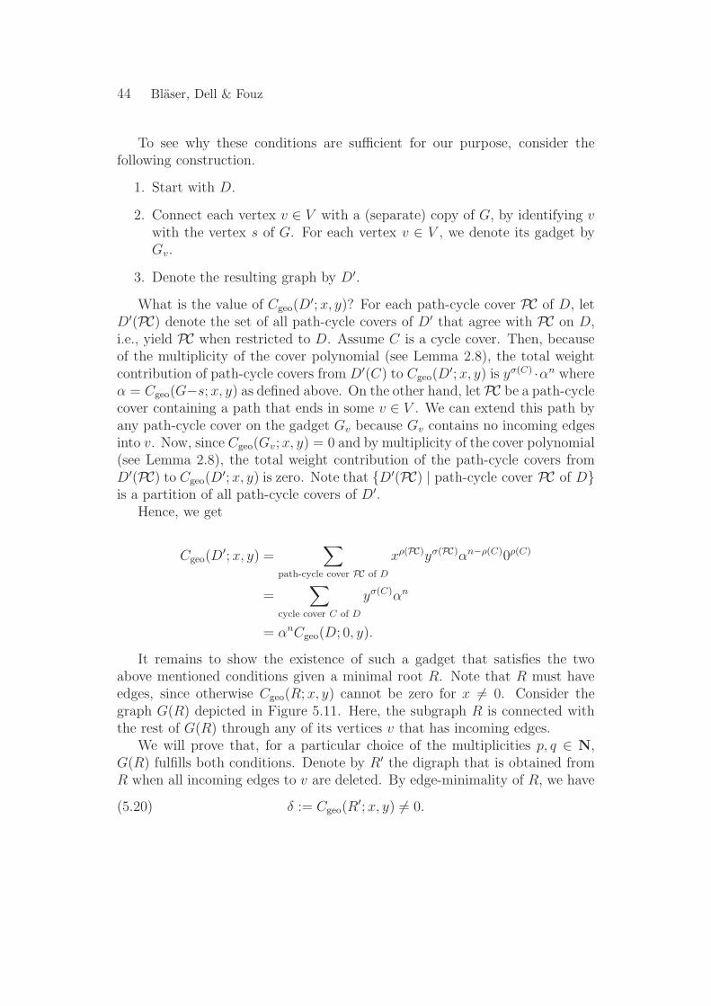
44 Blaser, Dell & Fouz
To see why these conditions are sufficient for our purpose, consider thefollowing construction.
1. Start with D.
2. Connect each vertex v ∈ V with a (separate) copy of G, by identifying vwith the vertex s of G. For each vertex v ∈ V , we denote its gadget byGv.
3. Denote the resulting graph by D′.
What is the value of Cgeo(D′; x, y)? For each path-cycle cover PC of D, let
D′(PC) denote the set of all path-cycle covers of D′ that agree with PC on D,i.e., yield PC when restricted to D. Assume C is a cycle cover. Then, becauseof the multiplicity of the cover polynomial (see Lemma 2.8), the total weightcontribution of path-cycle covers from D′(C) to Cgeo(D
′; x, y) is yσ(C) ·αn whereα = Cgeo(G−s; x, y) as defined above. On the other hand, let PC be a path-cyclecover containing a path that ends in some v ∈ V . We can extend this path byany path-cycle cover on the gadget Gv because Gv contains no incoming edgesinto v. Now, since Cgeo(Gv; x, y) = 0 and by multiplicity of the cover polynomial(see Lemma 2.8), the total weight contribution of the path-cycle covers fromD′(PC) to Cgeo(D
′; x, y) is zero. Note that {D′(PC) | path-cycle cover PC of D}is a partition of all path-cycle covers of D′.
Hence, we get
Cgeo(D′; x, y) =
∑
path-cycle cover PC of D
xρ(PC)yσ(PC)αn−ρ(C)0ρ(C)
=∑
cycle cover C of D
yσ(C)αn
= αnCgeo(D; 0, y).
It remains to show the existence of such a gadget that satisfies the twoabove mentioned conditions given a minimal root R. Note that R must haveedges, since otherwise Cgeo(R; x, y) cannot be zero for x 6= 0. Consider thegraph G(R) depicted in Figure 5.11. Here, the subgraph R is connected withthe rest of G(R) through any of its vertices v that has incoming edges.
We will prove that, for a particular choice of the multiplicities p, q ∈ N,G(R) fulfills both conditions. Denote by R′ the digraph that is obtained fromR when all incoming edges to v are deleted. By edge-minimality of R, we have
(5.20) δ := Cgeo(R′; x, y) 6= 0.
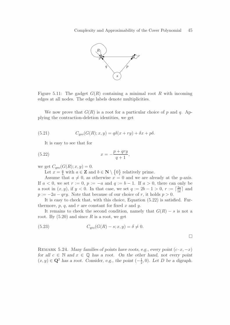
Complexity and Approximability of the Cover Polynomial 45
s
R
pq
vr
Figure 5.11: The gadget G(R) containing a minimal root R with incomingedges at all nodes. The edge labels denote multiplicities.
We now prove that G(R) is a root for a particular choice of p and q. Ap-plying the contraction-deletion identities, we get
Cgeo(G(R); x, y) = qδ(x + ry) + δx + pδ.(5.21)
It is easy to see that for
(5.22) x = −p + qry
q + 1,
we get Cgeo(G(R); x, y) = 0.Let x = a
bwith a ∈ Z and b ∈ N \
{
0}
relatively prime.Assume that a 6= 0, as otherwise x = 0 and we are already at the y-axis.
If a < 0, we set r := 0, p := −a and q := b − 1. If a > 0, there can only bea root in (x, y), if y < 0. In that case, we set q := 2b − 1 > 0, r := ⌈ 2a
|y|⌉ and
p := −2a − qry. Note that because of our choice of r, it holds p > 0.It is easy to check that, with this choice, Equation (5.22) is satisfied. Fur-
thermore, p, q, and r are constant for fixed x and y.It remains to check the second condition, namely that G(R) − s is not a
root. By (5.20) and since R is a root, we get
Cgeo(G(R) − s; x, y) = δ 6= 0.(5.23)
�
Remark 5.24. Many families of points have roots, e.g., every point (c ·x,−x)for all c ∈ N and x ∈ Q has a root. On the other hand, not every point(x, y) ∈ Q2 has a root. Consider, e.g., the point (−1
2, 0). Let D be a digraph.
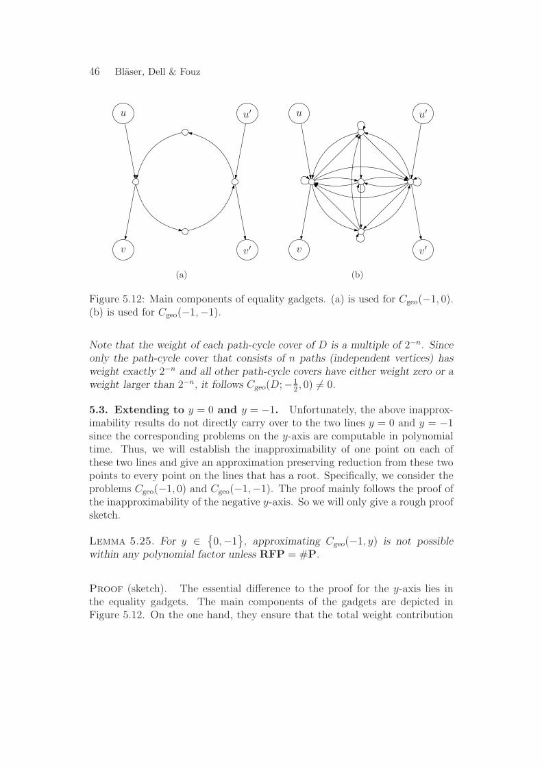
46 Blaser, Dell & Fouz
v
u
v′
u′
(a)
v
u
v′
u′
(b)
Figure 5.12: Main components of equality gadgets. (a) is used for Cgeo(−1, 0).(b) is used for Cgeo(−1,−1).
Note that the weight of each path-cycle cover of D is a multiple of 2−n. Sinceonly the path-cycle cover that consists of n paths (independent vertices) hasweight exactly 2−n and all other path-cycle covers have either weight zero or aweight larger than 2−n, it follows Cgeo(D;−1
2, 0) 6= 0.
5.3. Extending to y = 0 and y = −1. Unfortunately, the above inapprox-imability results do not directly carry over to the two lines y = 0 and y = −1since the corresponding problems on the y-axis are computable in polynomialtime. Thus, we will establish the inapproximability of one point on each ofthese two lines and give an approximation preserving reduction from these twopoints to every point on the lines that has a root. Specifically, we consider theproblems Cgeo(−1, 0) and Cgeo(−1,−1). The proof mainly follows the proof ofthe inapproximability of the negative y-axis. So we will only give a rough proofsketch.
Lemma 5.25. For y ∈{
0,−1}
, approximating Cgeo(−1, y) is not possiblewithin any polynomial factor unless RFP = #P.
Proof (sketch). The essential difference to the proof for the y-axis lies inthe equality gadgets. The main components of the gadgets are depicted inFigure 5.12. On the one hand, they ensure that the total weight contribution
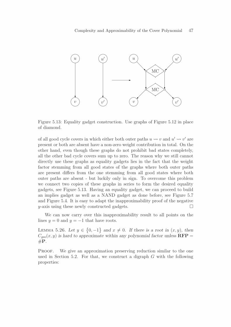
Complexity and Approximability of the Cover Polynomial 47
u
v
u′
v′
u
v
u′
v′
MC
MC
Figure 5.13: Equality gadget construction. Use graphs of Figure 5.12 in placeof diamond.
of all good cycle covers in which either both outer paths u v and u′ v′ arepresent or both are absent have a non-zero weight contribution in total. On theother hand, even though these graphs do not prohibit bad states completely,all the other bad cycle covers sum up to zero. The reason why we still cannotdirectly use these graphs as equality gadgets lies in the fact that the weightfactor stemming from all good states of the graphs where both outer pathsare present differs from the one stemming from all good states where bothouter paths are absent - but luckily only in sign. To overcome this problemwe connect two copies of these graphs in series to form the desired equalitygadgets, see Figure 5.13. Having an equality gadget, we can proceed to buildan implies gadget as well as a NAND gadget as done before, see Figure 5.7and Figure 5.4. It is easy to adapt the inapproximability proof of the negativey-axis using these newly constructed gadgets. �
We can now carry over this inapproximability result to all points on thelines y = 0 and y = −1 that have roots.
Lemma 5.26. Let y ∈{
0,−1}
and x 6= 0. If there is a root in (x, y), thenCgeo(x, y) is hard to approximate within any polynomial factor unless RFP =#P.
Proof. We give an approximation preserving reduction similar to the oneused in Section 5.2. For that, we construct a digraph G with the followingproperties:
48 Blaser, Dell & Fouz
1. G contains a vertex s with no incoming edges.
2. Cgeo(G; x, y) = −Cgeo(G − s; x, y) with α := Cgeo(G; x, y) 6= 0.
Using G in the same construction as in Section Section 5.2 and by the samereasoning, we get a digraph D′ with
Cgeo(D′; x, y) =
∑
path-cycle cover PC of D
αρ(PC)yσ(PC)(−α)n−ρ(PC)
= αn∑
path-cycle cover PC of D
(−1)ρ(PC)yσ(PC)
= αnCgeo(D;−1, y).
Given a minimal root R, we construct a digraph G(R) as shown in Fig-ure 5.11. As before, denote by R′ the graph that is obtained from R when allincoming edges to v are deleted. By edge-minimality of R, we have
(5.27) δ := Cgeo(R′; x, y) 6= 0.
We now prove Cgeo(G(R); x, y) = −Cgeo(G(R)− s; x, y) 6= 0 for a particularchoice of the multiplicities p, q ∈ N. By (5.21) we have,
Cgeo(G(R); x, y) = qδ(x + ry) + δx + pδ.(5.28)
Let x = ab
with a ∈ Z \{
0}
and b ∈ N \{
0}
relatively prime.If y = 0, there is no root in (x, y) for x > 0. It follows a < 0. By choosing
r := 0, q := b − 1 and p := −a + 1, we get Cgeo(G(R); x, y) = −δ. If y = −1,
let q := 2b− 1 > 0, r := ⌈2|a|q⌉ and p := qr − 2a − 1. Note that, because of our
choice of r, it holds p > 0 and Cgeo(G(R); x, y) = −δ.As for G(R) − s, we get by (5.23),
Cgeo(G(R) − s; x, y) 6= 0. �
6. Inapproximability of the Factorial Cover Polynomial
Although the cover polynomial agrees with the geometric cover polynomial onthe y-axis and satisfies the same contraction-deletion identities (2.7), except forthe base case, it seems much more difficult to handle than its geometric version.The reason is that while the geometric cover polynomial is multiplicative (seeLemma 2.8), we only have a rudimentary product rule for the cover polynomial.

Complexity and Approximability of the Cover Polynomial 49
Lemma 6.1 (Chung & Graham 1995, Corollary 2). Let D1,2 be the graph ob-tained as the disjoint union of two digraphs D1 = (V1, E1) and D2 = (V2, E2)together with all edges (v1, v2) for v1 ∈ V1 and v2 ∈ V2.
1 Then for all x, y ∈ Q,we have
C(D1,2, x, y) = C(D1, x, y)C(D2, x, y).
Interestingly, there is a nice relationship between the cover polynomial of asimple digraph D = (V, E) and its complement D = (V, V × V \ E).
Lemma 6.2 (Chung & Graham 1995, Chow 1996). Let D be a simple digraphand D its complement. It holds,
(6.3) C(D; x, y) = (−1)nC(D;−x − y, y).
The lack of proper multiplicativity makes the task of finding gadgets forapproximation preserving reductions harder than for the geometric cover poly-nomial. Still, since C agrees with the geometric cover polynomial on the y-axis,we get the following corollary.
Corollary 6.4. Let y ∈ Q with y /∈{
1, 0,−1}
.
For y > 0 or y < 0 approximating C(0, y) is not possible within any poly-nomial factor unless RP = NP or RFP = #P, respectively.
Note that this result also holds even if C(0, y) is restricted to simple graphs,since all reductions used either do not make any use of graphs with multipleedges or can be easily adjusted appropriately. We can extend it a bit by usingthe ‘horizontal reduction’ of (4.4) and the reciprocity formula of Lemma 6.2.
Corollary 6.5. Let y ∈ Q \{
1, 0,−1}
and c ∈ Z. For y > 0 or y < 0,C(c−y, y) and C(c, y) is not approximable within any polynomial factor, unlessRP = NP or RFP = #P, respectively.
Proof. Let r ∈ N. If C is restricted to simple graphs, we have
C(0, y) ≤AP C(r, y) by (4.4)
≤AP C(−r − y, y) by Lemma 6.2,
and furthermore,
1This is a kind of directed join.
50 Blaser, Dell & Fouz
C(0, y) ≤AP C(−y, y) by Lemma 6.2
≤AP C(r − y, y) by (4.4)
≤AP C(−r, y) by Lemma 6.2.
By setting r := c if c ≥ 0 and r := −c if c < 0, the corollary follows. �
7. Conclusion and Further Work
In this paper, we completely characterized the complexity of evaluating thecover polynomial and its geometric version in the rational plane. Our reductionsshould also work for complex or algebraic numbers, but we do not have anyinterpretation for such points yet.
We also gave a succinct characterization of a large class of points at whichapproximating the geometric cover polynomial within any polynomial factor isnot possible. Furthermore, we extended this result to a grid of points for thecover polynomial.
Further work is to be done until a full classification of inapproximable re-gions is achieved. Although we conjecture all points apart from the positivequadrant to be non-approximable, it is not clear at all whether such a resultcan be established by a reduction from the y-axis. As for the positive quadrant,the question of whether there exists, in general, an FPRAS seems wide open.Specifically, it is unclear whether the FPRAS for the line y = 1 (with x ≥ 0)also works for the whole positive quadrant. We tend to conjecture that apartfrom the line y = 1, only the line y = 0 is also approximable in the positivequadrant. As a step in this direction, one could try to prove that any FPRASsimilar to the one used for the line y = 1 is doomed to fail elsewhere in thisquadrant, in line with such a result for the independent set counting problemby Dyer et al. (2002).
One might conjecture that the connection between the Tutte and the coverpolynomial is solved because both are #P-hard to evaluate at most points,so they can be computed from each other (where they are in #P). From acombinatorial point of view, however, P-reductions are not really satisfyingsteps towards a deeper understanding of the connection between the two graphpolynomials.
One promising approach might be to consider generalizations of the coverpolynomial. Very recently, Courcelle (unpublished) analyzed general contraction-deletion identities analogous to those of the coloured Tutte polynomial, and hefound conditions for the variables which are necessary and sufficient for the
Complexity and Approximability of the Cover Polynomial 51
well-definedness of the polynomial. Unfortunately, these conditions seem toorestrictive.
The contraction-deletion identities of Tutte and cover polynomial look as-tonishingly similar, but contractions work differently for directed and for undi-rected graphs. Explaining the connection between Tutte and cover polynomialmeans overcoming this difference.
Acknowledgements
We would like to thank Thomas Jansen and Moritz Hardt for fruitful discussionsand valuable remarks on earlier versions of this paper. We would also like tothank the referees for their helpful comments.
Research of the second author supported by the Deutsche Forschungsge-meinschaft within the research training group Methods for Discrete Structures(GRK 1408).
References
Artur Andrzejak (1998). An algorithm for the Tutte polynomials of graphs ofbounded treewidth. Discrete Mathematics 190(1-3), 39–54.
Ilia Averbouch, Benny Godlin & Johann A. Makowsky (2008). A MostGeneral Edge Elimination Polynomial. In Graph-Theoretic Concepts in ComputerScience, 34th International Workshop, WG 2008, Durham, UK, June 30 - July 2,2008. Revised Papers, volume 5344 of Lecture Notes in Computer Science, 31–42.
Andreas Bjorklund, Thore Husfeldt, Petteri Kaski & Mikko Koivisto
(2008). Computing the Tutte polynomial in vertex-exponential time.
Markus Blaser, Holger Dell & Johann A. Makowsky (2008). Complexity ofthe Bollobas-Riordan Polynomial. In 3rd International Computer Science Symposiumin Russia (CSR), 86–98.
Markus Blaser & Christian Hoffmann (2008). On the Complexity of the Inter-lace Polynomial. In 25th International Symposium on Theoretical Aspects of Com-puter Science (STACS 2008), Susanne Albers & Pascal Weil, editors, 97–108.Internationales Begegnungs- und Forschungszentrum fur Informatik (IBFI), SchlossDagstuhl, Germany, Dagstuhl, Germany. URL http://drops.dagstuhl.de/opus/
volltexte/2008/1337.
Markus Blaser & Christian Hoffmann (2009). Fast Evaluation of InterlacePolynomials on Graphs of Bounded Treewidth. In Algorithms - ESA 2009, 17th

52 Blaser, Dell & Fouz
Annual European Symposium, volume 5757 of Lecture Notes in Computer Science,623–634. Springer.
Lenore Blum, Felipe Cucker, Michael Shub & Steve Smale (1998). Com-plexity and real computation. Springer-Verlag New York, Inc., Secaucus, NJ, USA.ISBN 0-387-98281-7.
Bela Bollobas & Oliver Riordan (1999). A Tutte Polynomial for ColouredGraphs. Combinatorics, Probability and Computing 8(1-2), 45–93.
Andrei Bulatov & Martin Grohe (2005). The complexity of partition functions.Theoretical Computer Science 348(2), 148–186.
Timothy Y. Chow (1996). A Short Proof of the Rook Reciprocity Theorem. Electr.J. Comb. 3(1).
Fan R.K. Chung & Ronald L. Graham (1995). On the cover polynomial of adigraph. Journal of Combinatorial Theory Series B 65(2), 273–290.
Bruno Courcelle, Johann A. Makowsky & Udi Rotics (2001). On the fixedparameter complexity of graph enumeration problems definable in monadic second-order logic. Discrete Applied Mathematics 108(1-2), 23–52.
Ottavio M. D’Antona & Emanuele Munarini (2000). The cycle-path indicatorpolynomial of a digraph. Adv. Appl. Math. 25(1), 41–56.
Martin Dyer, Alan Frieze & Mark Jerrum (2002). On Counting IndependentSets in Sparse Graphs. SICOMP: SIAM Journal on Computing 31.
Martin E. Dyer, Alan M. Frieze & Mark Jerrum (1998). ApproximatelyCounting Hamilton Paths and Cycles in Dense Graphs. SIAM Journal on Computing27(5), 1262–1272.
Martin E. Dyer, Leslie Ann Goldberg & Mike Paterson (2006). On Count-ing Homomorphisms to Directed Acyclic Graphs. In Proceedings of the 33rd Interna-tional Colloquium on Automata, Languages and Programming, ICALP 2006, volume4051 of Lecture Notes in Computer Science, 38–49. Springer.
Michael R. Garey & David S. Johnson (1979). Computers and Intractability.Freeman, San Francisco.
Omer Gimenez & Marc Noy (2006). On the Complexity of Computing the TuttePolynomial of Bicircular Matroids. Combinatorics, Probability and Computing 15(3),385–395.
Complexity and Approximability of the Cover Polynomial 53
Leslie Ann Goldberg & Mark Jerrum (2008). Inapproximability of the Tuttepolynomial. Inform. Comput. 206(7), 908–929.
Christian Hoffmann (2010). A Most General Edge Elimination Polynomial -Thickening of Edges. Fundam. Inform. 98(4), 373–378.
Francois Jaeger, Dirk L. Vertigan & Dominic J.A. Welsh (1990). On thecomputational complexity of the Jones and Tutte polynomials. Mathematical Pro-ceedings of the Cambridge Philosophical Society 108(1), 35–53.
Mark Jerrum & Alistair Sinclair (1989). Approximate Counting, Uniform Gen-eration and Rapidly Mixing Markov Chains. Information and Computation 82(1),93–133.
Mark Jerrum & Alistair Sinclair (1997). The Markov Chain Monte CarloMethod: An Approach to Approximate Counting and Integration. In ApproximationAlgorithms for NP-hard Problems, D. Hochbaum, editor. PWS Publishing Com-pany.
Mark Jerrum, Alistair Sinclair & Eric Vigoda (2004). A Polynomial-TimeApproximation Algorithm for the Permanent of a Matrix with Nonnegative Entries.JACM: Journal of the ACM 51.
Nathan Linial (1986). Hard enumeration problems in geometry and combinatorics.SIAM J. Algebraic Discrete Methods 7(2), 331–335.
Martin Lotz & Johann A. Makowsky (2004). On the algebraic complexityof some families of coloured Tutte polynomials. Advances in Applied Mathematics32(1), 327–349.
Johann A. Makowsky (2008). From a zoo to a zoology: Towards a general theoryof graph polynomials. Theory of Computing Systems 43(3), 542–562.
S. D. Noble (1998). Evaluating the Tutte Polynomial for Graphs of Bounded Tree-Width. Combinatorics, Probability & Computing 7(3), 307–321.
Christos M. Papadimitriou (1994). Computational Complexity. Addison-Wesley,Reading, Massachusetts.
Leslie G. Valiant (1979). The complexity of computing the permanent. Theoret-ical Computer Science 8(2), 189–201.
Leslie G. Valiant & Vijay V. Vazirani (1986). NP is as easy as detecting uniquesolutions. Theoretical Computer Science 47(1), 85–93.

54 Blaser, Dell & Fouz
Manuscript received 7 November 2008
Markus Blaser
Department of Computer ScienceSaarland UniversitySaarbrucken, [email protected]
Holger Dell
Department of Computer ScienceHumboldt University of BerlinBerlin, [email protected]
Mahmoud Fouz
Department of Computer ScienceSaarland UniversitySaarbrucken, [email protected]