approximability of integer programming with generalised ... · approximability of integer...
TRANSCRIPT
arX
iv:c
s/06
0204
7v1
[cs.
CC
] 13
Feb
200
6
Approximability of Integer Programming with
Generalised Constraints
Peter Jonsson⋆, Fredrik Kuivinen⋆⋆, and Gustav Nordh⋆ ⋆ ⋆
Department of Computer and Information ScienceLinkopings Universitet
S-581 83 Linkoping, Sweden{petej, freku, gusno}@ida.liu.se
Abstract
Given a set of variables and a set of linear inequalities over those vari-ables, the objective in the Integer Linear Programming problem is tofind an integer assignment to the variables such that the inequalities aresatisfied and a linear goal function is maximised. We study a family ofproblems, called Maximum Solution, which are related to Integer Lin-ear Programming. In a Maximum Solution problem, the constraintsare drawn from a set of allowed relations, hence arbitrary constraints arestudied instead of just linear inequalities. When the domain is Boolean(i.e. restricted to {0, 1}), the maximum solution problem is identical to thewell-studied Max Ones problem, and the approximability is completelyunderstood for all restrictions on the underlying constraints [Khanna etal., SIAM J. Comput., 30 (2000), pp. 1863-1920]. We continue this lineof research by considering domains containing more than two elements.Our main results are two new large tractable fragments for the maximumsolution problem and a complete classification for the approximability ofall maximal constraint languages. Moreover, we give a complete classi-fication of the approximability of the problem when the set of allowedconstraints contains all permutation constraints. Our results are provedby using algebraic results from clone theory and the results indicates thatthis approach is very useful for classifying the approximability of certainoptimisation problems.
Classification: Computational and structural complexity; Approximability
1 Introduction
Combinatorial optimisation problems can often be formulated as integer linearprograms. In its most general form the aim in a integer linear program is toassign integers to a set of variables such that a set of linear inequalities aresatisfied and a linear goal function is maximised or minimised. In this generalform of the problem it is NP-hard to find feasible solutions [14]. It is well-known
⋆Partially supported by the Center for Industrial Information Technology (CENIIT) undergrant 04.01, and by the Swedish Research Council (VR) under grant 621-2003-3421.
⋆⋆Supported by the Swedish Research Council (VR) under grant 621-2002-4126.⋆ ⋆ ⋆Supported by the National Graduate School in Computer Science (CUGS), Sweden.
1. Introduction 2
that restrictions to the general integer linear programming problem still has theability to express many real-world optimisation problems. One such restrictionis to only consider solutions consisting of 0 and 1, i.e., the domain is {0, 1}. Thisproblem, commonly called Maximum 0-1 Programming, is still very hard, infact it is NPO-complete [20].
If certain restrictions are placed on the constraints (e.g., the constraint ma-trix is totally unimodular) in an Integer Linear Programming (here afterabbreviated as ILP) instance the optimum will coincide with the optimum forthe corresponding Linear Programming instance, this restricted set of prob-lems are thus solvable in polynomial time [27]. Other restrictions of the ILPproblem have also been studied, e.g., Hochbaum and Naor [15], give pseudo-polynomial time algorithms for ILP when we have at most two variables perinequality.
If one disallows integer constraints, i.e., the domain of every variable is thereals then the ILP problem becomes the well-known Linear Programmingproblem. Linear Programming can be solved in polynomial time with, forexample, the ellipsoid algorithm [27].
In this paper we study generalisations of the linear integer programmingproblem in the sense that we allow arbitrary sets of relations as our constraints.Our goal is to classify the complexity of obtaining approximate solutions to thisproblem for all different sets of allowed constraints. We approach this problemfrom the constraint satisfaction angle. A wide range of combinatorial problemscan be viewed as ‘constraint satisfaction problems’ (CSPs), in which the aimis to find an assignment of values to a set of variables subject to certain con-straints. Typical examples include the satisfiability problem, graph colourabilityproblems and many others. As stated above, we study a certain optimisationproblem which is derived from CSPs: we do not only want to determine whetherthere exists a solution or not, but also to find a solution which maximises thesum of the variables.
Let us begin by formally defining this problem: Let D ⊂ N (the domain) bea finite set. The set of all n-tuples of elements from D is denoted by Dn. Anysubset ofDn is called an n-ary relation onD. The set of all finitary relations overD is denoted by RD. A constraint language over a finite set, D, is a finite setΓ ⊆ RD. Constraint languages are the way in which we specify restrictions onour problems. The constraint satisfaction problem over the constraint languageΓ, denotedCsp(Γ), is defined to be the decision problem with instance (V,D,C),where
• V is a set of variables,
• D is a finite set of values (sometimes called a domain), and
• C is a set of constraints {C1, . . . , Cq}, in which each constraint Ci is apair (si, i) with si a list of variables of length mi, called the constraintscope, and i an mi-ary relation over the set D, belonging to Γ, called theconstraint relation.
1. Introduction 3
The question is whether there exists a solution to (V,D,C) or not, that is, afunction from V to D such that, for each constraint in C, the image of theconstraint scope is a member of the constraint relation.
To exemplify this definition, let NAE be the following ternary relationon {0, 1}: NAE = {0, 1}3 \ {(0, 0, 0), (1, 1, 1)}. It is easy to see that thewell-known NP-complete problem Not-All-Equal Sat can be expressed asCsp({NAE}).
The optimisation we are going to study, Weighted Maximum Solution,can then be defined as follows:
Definition 1.1 Weighted Maximum Solution over the constraint languageΓ, denoted W-Max Sol(Γ), is defined to be the optimisation problem with
Instance: Tuple (V,D,C,w), where D is a finite subset of N, (V,D,C) is aCsp instance over Γ, and w : V → N is a weight function.
Solution: An assignment f : V → D to the variables such that all constraintsare satisfied.
Measure:∑
v∈V
w(v) · f(v)
We remark in passing that non-trivial exponential-time algorithms for W-MaxSol have recently been presented in [2, 3]. The problem W-Max Sol shouldnot be confused with the Max Csp problem where the objective is to maximisethe number of satisfied constraints. The approximability of this problem iscurrently an active research area and recent results include a dichotomy theoremfor three-element domains [21]. We note that these results are achieved by usingcompletely different methods than those that will be used in this paper. In fact,it is known that the algebraic approach that we will use is basically useless forproving properties of the Max Csp problem.
W-Max Sol restricted to Boolean domains is known as Weighted MaxOnes and the approximability of (Weighted) Max Ones is completely under-stood for all constraint languages [22]: For any Boolean constraint language Γ,W-Max Sol(Γ) is either in PO or is APX-complete or poly-APX-completeor finding a solution of non-zero value is NP-hard or finding any solution is NP-hard. The exact borderlines between the different cases is given in [22] where itis also proved that the borderlines for the weighted and unweighted versions ofthe problem coincide. We remark that the same result holds for all constraintlanguages considered in this paper (i.e., the approximability of the weighted andunweighted versions of the problem agrees for all maximal constraint languagesand constraint languages containing all permutation relations).
While the approximability ofW-Max Sol is well-understood for the Booleandomain, this is not the case for larger domains. For larger domains we are awareof two results, the first one is a tight (in)approximability results for W-MaxSol(Γ) when Γ is the set of relations that can be expressed as linear equationsover Zp [23]. The second result is due to Hochbaum and Naor [15], they studyinteger programming with monotone constraints, i.e., every constraint is of the
2. Preliminaries 4
form ax − by ≤ c, where x and y are variables and a, b ∈ N and c ∈ Z. Inour setting their result is a polynomial time algorithm for certain constraintlanguages. It is worth pointing out that restricting the ILP-problem to totallyunimodular matrices do not give tractability results for W-Max Sol. Thisis because the totally unimodular restriction is not purely a restriction on theconstraint language, it is also a restriction on how the constraints are appliedto the variables. The main goal of this paper is to try to remedy this situationby showing how the algebraic approach for CSPs [7, 19] can be used to studythe approximability of W-Max Sol.
The algebraic approach to the study of the complexity of CSPs has beenvery successful: it has, for instance, made it possible to design new efficientalgorithms and to clarify the borderline between tractability and intractabilityin many important cases. In particular the complexity of the CSP problem overthree element domains is now completely understood [5]. By using this algebraicapproach we are able to present the following three main results:
Result 1. We identify two new large tractable classes of W-Max Sol(Γ): in-jective constraints and generalised max-closed constraints. These two classessignificantly extends the non-trivial tractable classes of Max Ones that wereidentified by Khanna et al. By using the theory for homogeneous algebras,we additionally prove that the class of injective constraints ΓP is a maximallytractable class, i.e. W-Max Sol(ΓP ∪ {r}) is not tractable whenever r 6∈ ΓP
(unless P = NP).
Result 2. We completely characterise the approximability of maximal con-straint languages; a constraint language Γ is maximal if, for any r 6∈ Γ, Γ ∪ {r}has the ability to express (in a sense to be formally defined later on) every re-lation in RD. Such languages have attracted much attention lately [6, 8]. Ourresults shows that if Γ is maximal, then W-Max Sol(Γ) is either tractable,APX-complete, poly-APX-complete, or that finding any solution with non-zero measure is NP-hard. The different cases can also be efficiently recognisedgiven an arbitrary maximal constraint language.
Result 3. We completely classify the approximability of constraint languagesthat contain all permutation relations. The proof of this result heavily relies onthe structure of homogeneous algebras. Dalmau [12] has proved a dichotomytheorem for the satisfiability problem on this set of relations.
The paper is structured as follows: Section 2 contains some basics on approxima-bility and the algebraic approach to CSPs and Section 3 identifies certain hardconstraint languages. Section 4 contains Result 1, Section 5 contains Result2 and Section 6 contains Result 3. Section 7 contains some final remarks.
2 Preliminaries
In this section we state some preliminaries which we will need throughout thepaper.
2.1. Approximability, Reductions, and Completeness 5
For a relation R with arity a we will sometimes write R(x1, . . . , xa) withthe meaning (x1, . . . , xa) ∈ R. Furthermore, the constraint ((x1, . . . , xa), R)will sometimes be written as R(x1, . . . , xa). The intended meaning will be clearfrom the context. Given an instance I = (V,D,C) of a Csp-problem we definethe constraint graph of I to be G = (V,E) where {v, v′} ∈ E if there is at leastone constraint c ∈ C which have both v and v′ in its constraint scope.
2.1 Approximability, Reductions, and Completeness
A combinatorial optimisation problem is defined over a set of instances (admis-sible input data); each instance I has a finite set sol(I) of feasible solutionsassociated with it. The objective is, given an instance I, to find a feasible solu-tion of optimum value with respect to some measure function m : sol(I) → N.The optimal value is the largest one for maximisation problems and the small-est one for minimisation problems. A combinatorial optimisation problem issaid to be an NPO problem if its instances and solutions can be recognised inpolynomial time, the solutions are polynomial-bounded in the input size, andthe objective function can be computed in polynomial time (see, e.g., [4]).
Definition 2.1 A solution s ∈ sol(I) to an instance I of an NPO problem Πis r-approximate if it is satisfying
max
{m(s)
opt(I),opt(I)
m(s)
}
≤ r,
where opt(I) is the optimal value for a solution to I. An approximation algo-rithm for an NPO problem Π has performance ratio R(n) if, given any instanceI of Π with |I| = n, it outputs an R(n)-approximate solution.
Definition 2.2 PO is the class of NPO problems that can be solved (to opti-mality) in polynomial time. An NPO problem Π is in the class APX if thereis a polynomial-time approximation algorithm for Π whose performance ratiois bounded by a constant. Similarly, Π is in the class poly-APX if there isa polynomial-time approximation algorithm for Π whose performance ratio isbounded by a polynomial in the size of the input.
Completeness in APX and poly-APX is defined using an appropriate re-duction, called AP -reduction [11, 22].
Definition 2.3 An NPO problem Π1 is said to be AP -reducible to an NPOproblem Π2 if two polynomial-time computable functions F and G and a constantα exist such that
(a) for any instance I of Π1, F (I) is an instance of Π2;
(b) for any instance I of Π1, and any feasible solution s′ of F (I), G(I, s′) isa feasible solution of I;
2.2. Algebraic Approach to CSPs 6
(c) for any instance I of Π1, and any r ≥ 1, if s′ is an r-approximate solutionof F (I) then G(I, s′) is an (1 + (r − 1)α + o(1))-approximate solution ofI where the o-notation is with respect to |I|.
An NPO problem Π is APX-hard (poly-APX-hard) if every problem inAPX (poly-APX) is AP -reducible to it. If, in addition, Π is in APX (poly-APX), then Π is called APX-complete (poly-APX-complete).
It is a well-known fact (see, e.g., Section 8.2.1 in [4]) that AP -reductions com-pose. In some proofs we will use another kind of reduction, S-reductions. Theyare defined as follows:
Definition 2.4 An NPO problem Π1 is said to be S-reducible to an NPOproblem Π2 if two polynomial-time computable functions F and G exist suchthat
(a) given any instance I of Π1, algorithm F produces an instance I ′ = F (I)of Π2, such that the measure of an optimal solution for I ′, opt(I ′), isexactly opt(I).
(b) given I ′ = F (I), and any solution s′ to I ′, algorithm G produces a solutions to I such that m(G(s′)) = m′(s′).
Obviously, the existence of an S-reduction from Π1 to Π2 implies the existenceof an AP -reduction from Π1 to Π2. The reason why we need S-reductions isthat AP -reductions do not (generally) preserve membership in PO [22].
In some of our hardness proofs, it will be convenient for us to use a type ofapproximation-preserving reduction called L-reduction [4].
Definition 2.5 An NPO problem Π1 is said to be L-reducible to an NPOproblem Π2 if two polynomial-time computable functions F and G and positiveconstants β and γ exist such that
(a) given any instance I of Π1, algorithm F produces an instance I ′ = F (I)of Π2, such that the measure of an optimal solution for I ′, opt(I ′), is atmost β · opt(I);
(b) given I ′ = F (I), and any solution s′ to I ′, algorithm G produces a solutions to I such that |m1(s) − opt(I)| ≤ γ · |m2(s
′) − opt(I ′)|, where m1 isthe measure for Π1 and m2 is the measure for Π2.
It is well-known (see, e.g., Lemma 8.2 in [4]) that, if Π1 is L-reducible to Π2
and Π1 ∈ APX then there is an AP -reduction from Π1 to Π2.
2.2 Algebraic Approach to CSPs
An operation on a finite setD (the domain) is an arbitrary function f : Dk → D.Any operation on D can be extended in a standard way to an operation on tu-ples over D, as follows: Let f be a k-ary operation on D and let R be an n-ary
2.2. Algebraic Approach to CSPs 7
relation over D. For any collection of k tuples, t1, t2, . . . , tk ∈ R, the n-tuplef(t1, t2, . . . , tk) is defined as follows: f(t1, t2, . . . , tk) = (f(t1[1], t2[1], . . . , tk[1]),f(t1[2], t2[2], . . . , tk[2]), . . . , f(t1[n], t2[n], . . . , tk[n])), where tj [i] is the i-th com-ponent in tuple tj . A technique that has shown to be useful in determining thecomputational complexity of Csp(Γ) is that of investigating whether Γ is invari-ant under certain families of operations [19].
Definition 2.6 Let i ∈ Γ. If f is an operation such that for all t1, t2, . . . , tk ∈i f(t1, t2, . . . , tk) ∈ i, then i is invariant (or, in other words, closed) underf . If all constraint relations in Γ are invariant under f then Γ is invariant underf . An operation f such that Γ is invariant under f is called a polymorphismof Γ. The set of all polymorphisms of Γ is denoted Pol(Γ). Given a set ofoperations F , the set of all relations that is invariant under all the operationsin F is denoted Inv(F ).
We will need a number of operations in the sequel:
Definition 2.7 An operation f over D is said to be
• a constant operation if f is unary and f(a) = c for all a ∈ D and somec ∈ D;
• a majority operation if f is ternary and f(a, a, b) = f(a, b, a) = f(b, a, a) =a for all a, b ∈ D;
• binary commutative idempotent operation if f is binary, f(a, a) = a forall a ∈ D, and f(a, b) = f(b, a) for all a, b ∈ D;
• an affine operation if f is ternary and f(a, b, c) = a−b+c for all a, b, c ∈ Dwhere + and − are the binary operations of an Abelian group (D,+,−).
The definitions above can be exemplified as follows:
Example 2.1 Let D = {0, 1, 2} and let f be the majority operation on D wheref(a, b, c) = a if a, b and c are all distinct. Furthermore, let
R = {(0, 0, 1), (1, 0, 0), (2, 1, 1), (2, 0, 1), (1, 0, 1)}.
It is then easy to verify that for every triple of tuples, x,y, z ∈ R, we havef(x,y, z) ∈ R. For example, if x = (0, 0, 1),y = (2, 1, 1) and z = (1, 0, 1) then
f(x,y, z) =
(
f(x[1],y[1], z[1]), f(x[2],y[2], z[2]), f(x[3],y[3], z[3])
)
=
(f(0, 2, 1), f(0, 1, 0), f(1, 1, 1)
)= (0, 0, 1) ∈ R.
We can conclude that R is invariant under f , or equivalently f is a polymor-phism of R.
2.2. Algebraic Approach to CSPs 8
We continue by defining a closure operation 〈·〉 on sets of relations: for anyset Γ ⊆ RD the set 〈Γ〉 consists of all relations that can be expressed usingrelations from Γ ∪ {=D} (=D is the equality relation on D), conjunction, andexistential quantification. Intuitively, constraints using relations from 〈Γ〉 areexactly those which can be simulated by constraints using relations from Γ.The sets of relations of the form 〈Γ〉 are referred to as relational clones, orco-clones. An alternative characterisation of relational clones is given in thefollowing theorem.
Theorem 2.8 ([26]) For every set Γ ⊆ RD, 〈Γ〉 = Inv(Pol(Γ)).
The following theorem states that when we are studying the approximabilityof W-Max Sol(Γ) it is sufficient to consider constraint languages that arerelational clones.
Theorem 2.9 Let Γ be a finite constraint language and Γ′ ⊆ 〈Γ〉 finite. ThenW-Max Sol(Γ′) is S-reducible to W-Max Sol(Γ).
Proof. Consider an instance I = (V,D,C,w) ofW-Max Sol(Γ′). We transformI into an instance F (I) = (V ′, D,C′, w′) of W-Max Sol(Γ).
For every constraint C = ((v1, . . . , vm), ) in I, can be represented as
∃vm+1, . . . , ∃vn1(v11, . . . , v1n1
) ∧ · · · ∧ k(vk1, . . . , vknk)
where 1, . . . , k ∈ Γ∪{=D}, vm+1, . . . , vn are fresh variables, and v11, . . . , v1n1,
v21, . . . , vknk∈ {v1, . . . , vn}. Replace the constraint C with the constraints
((v11, . . . , v1n1), 1), . . . , ((vk1, . . . , vknk
), k), add vm+1, . . . , vn to V , and extendw so that vm+1, . . . vn are given weight 0. If we repeat the same reduction forevery constraint in C it results in an equivalent instance of W-Max Sol(Γ1 ∪{=D}).
For each equality constraint ((vi, vj),=D) we do the following:
• If vj occurs in another constraint, then replace all occurrences of vj withvi, update w
′ so that the weight of vj is added to the weight of vi, removevj from V , and remove the weight corresponding to vj from w′.
• Finally remove ((vi, vj),=D) from C.
The resulting instance F (I) = (V ′, D,C′, w′) of W-Max Sol(Γ) has the sameoptimum as I (i.e., opt(I) = opt(F (I))) and has been obtained in polynomialtime.
Now, given a feasible solution S′ for F (I), let G(I, S′) be the feasible solutionfor I where:
• The variables in I assigned by S′ inherit their value from S′.
• The variables in I which are still unassigned all occur in equality con-straints and their values can be found by simply propagating the valuesof the variables which have already been assigned.
3. Hardness and General Containment Results 9
It should be clear that m(I,G(I, S′)) = m(F (I), S′) for any feasible solutionS′ for F (I). Hence, the functions F and G, as described above, is an S-reductionfrom W-Max Sol(Γ′) to W-Max Sol(Γ). ⊓⊔
3 Hardness and General Containment Results
In this section we prove some general containment results in APX and poly-APX for W-Max Sol(Γ). We also prove APX-completeness and poly-APX-completeness for W-Max Sol(Γ) for some particular constraint languages Γ.Most of our hardness results in subsequent sections are based on these results.
We begin by making the following easy but interesting observation: we knowfrom the classification of W-Max Sol(Γ) over the Boolean domain {0, 1} thatthere exist many constraint languages Γ for which W-Max Sol(Γ) is poly-APX-complete. However, if 0 is not in the domain, then there are no constraintlanguages Γ such that W-Max Sol(Γ) is poly-APX-complete.
Proposition 3.1 If Csp(Γ) is in P and 0 /∈ D, then W-Max Sol(Γ) is inAPX.
Proof. It is proved in [9] that if Csp(Γ) is in P, then we can also find a solution
in polynomial time. It should be clear that this solution is a max(D)min(D) -approximate
solution. Hence we have a trivial approximation algorithm with performance
ratio max(D)min(D) . ⊓⊔
Next we present a general containment result in poly-APX for W-MaxSol(Γ). The proof is similar to the proof of the corresponding result for theBoolean domain in [22, Lemma 6.2], so we omit the proof.
Lemma 3.2 Let Γc = {Γ∪ {{(d1)}, . . . , {(dn)}}, where D = {d1, . . . , dn} (i.e.,Γc is the constraint language corresponding to Γ where we can force variables totake any given value in the domain). If Csp(Γc) is in P, then W-Max Sol(Γ)is in poly-APX.
As for the hardness results, we begin by proving the APX-completenessof particular constraint languages that will be very useful for obtaining APX-completeness results in subsequent sections.
Lemma 3.3 Let r = {(a, a), (a, b), (b, a)} and a, b ∈ D such that 0 < a < b.Then, W-Max Sol({r}) is APX-complete.
Proof. We give an L-reduction (with β = 4b and γ = 1b−a
) from the APX-complete problem Independent Set restricted to degree 3 graphs [1] to MaxSol({r}). Given an instance I = (V,E) of Independent Set (restricted tographs of degree at most 3 and containing no isolated vertices), let F (I) =(V,D,C) be the instance of Max Sol({r}) where, for each edge (vi, vj) ∈ E,we add the constraint r(xi, xj) to C. For any feasible solution S′ for F (I),let G(I, S′) be the solution for I where all vertices corresponding to variables
4. Tractable Constraint Languages 10
assigned b in S′ form the independent set. We have |V |/4 ≤ opt(I) andopt(F (I)) ≤ b|V |, hence opt(F (I)) ≤ 4bopt(I). Thus, β = 4b is an ap-propriate parameter.
Let K be the number of variables being set to b in an arbitrary solution S′
for F (I). Then,
|opt(I)−m(I,G(I, S′))| = opt(I)−K, and
|opt(F (I))−m(F (I), S′)| = (b− a)(opt(I)−K).
Hence,
|opt(I)−m(I,G(I, S′)| =1
b− a|opt(F (I)) −m(F (I), S′)|
and γ = 1b−a
is an appropriate parameter.This L-reduction ensures that Max Sol({r}) is APX-hard. ⊓⊔
The generic poly-APX-complete constraint languages are presented in thefollowing lemma.
Lemma 3.4 Let r = {(0, 0), (0, b), (b, 0)} and b ∈ D such that 0 < b. Then,W-Max Sol({r}) is poly-APX-complete.
Proof. It is proved in [22, Lemma 6.15] that for s = {(0, 0), (0, 1), (1, 0)}, it isthe case that W-Max Sol({s}) is poly-APX-complete. To prove the poly-APX-hardness we give an AP -reduction from W-Max Sol({s}) to W-MaxSol({r}). Given an instance I of W-Max Sol({s}), let F (I) be the instanceof W-Max Sol({r}) where all occurrences of s has been replaced by r. Forany feasible solution S′ for F (I), let G(I, S′) be the solution for I where allvariables assigned a in S′ are instead assigned 1. It should be clear that this isa AP -reduction, since if S′ is a r-approximate solution to F (I), then G(I, S′) ar-approximate solution for I.
To see that W-Max Sol({r}) is in poly-APX, let D = {d1, . . . , dn}and note that for Γc = {r, {(d1)}, . . . , {(dn)}}, Γ
c is invariant under the min-function. As the min-function is associative, commutative and idempotentCsp(Γc) is solvable in polynomial time [19]. Hence, due to Lemma 3.2 W-Max Sol({r}) is in poly-APX. ⊓⊔
4 Tractable Constraint Languages
In this section, we identify two large new tractable (in PO) classes of constraintlanguages for the W-Max Sol(Γ) problem. The new tractable classes are injec-tive constraint languages and generalised max-closed constraint languages. Tothe best of our knowledge, these two classes subsumes all the known tractableclasses of constraint languages presented in the literature for this problem. Inparticular, they can be seen as substantial and nontrivial generalisations ofthe tractable classes known for the corresponding (Weighted) Max Ones
4.1. Injective Relations 11
problem over the Boolean domain. There are only three tractable classes ofconstraint languages over the Boolean domain, namely width-2 affine, 1-valid,and weakly positive [22]. Width-2 affine constraint languages are examples ofinjective constraint languages and the classes of 1-valid and weakly positive con-straint languages are examples of generalised max-closed constraint languages.The monotone constraints, studied by Woeginger [30] and by Hochbaum andNaor [15] in relation to Integer Programming, are also a subset of the gen-eralised max-closed constraints studied in this paper.
We note that the injective constraints is a special class of 0/1/all constraintsas defined in [10]. It is proved in [10] that the class of 0/1/all constraints is amaximal tractable class for the Csp problem. This means that if Γ consists ofall relations corresponding to 0/1/all constraints, and R is any relation which isnot 0/1/all, then Csp(Γ ∪ {R}) is NP-complete. We prove an analogous resultin Section 6, namely that the class of injective constraints is a maximal tractableclass for the W-Max Sol problem.
4.1 Injective Relations
In this section we will prove the tractability of W-Max Sol(F ) when F is ainjective set of relations. Injective relations are defined as follows:
Definition 4.1 A relation, R ∈ RD, is called injective if there exists a subsetD′ ⊆ D and an injective function π : D′ → D such that R = {(x, π(x)) | x ∈ D′}.
It is important to note that the function π is not assumed to be total on D.Let ID denote the set of all injective relations on the domain D and let
ΓDI = 〈ID〉.
Example 4.1 Let D = {0, 1} and let R = {(x, y) | x, y ∈ D, x+y ≡ 1 mod 2}.R is injective because the function f : D → D defined as f(0) = 1 and f(1) = 0is injective.
More generally, let G = (D′,+,−) be an arbitrary Abelian group and letc ∈ D′ be an arbitrary group element it is then easy to see that the relation{(x, y) | x, y ∈ D′, x+ y = c} is injective.
R is an example of a relation which is invariant under an affine operation. Suchrelations have previously been studied in relation with the Max Sol problemin [23]. We will give some additional results for such constraints in Section 5.3.With the terminology used in [23] R is said to be width-2 affine.
The relations which can be expressed as the set of solutions to an equationwith two variables over an Abelian group are exactly the width-2 affine relationsin [23], hence the injective relations are a superset of the width-2 affine relations.
Lemma 4.2 W-Max Sol(ΓDI ) is in PO.
Proof. By Theorem 2.9, it is sufficient to prove the tractability of W-MaxSol(ID), where ΓD
I = 〈ID〉 and ID is a set of all constraints which are injective.
4.2. Generalised Max-Closed Relations 12
Let I = (V,D,C,w) be an arbitrary instance of W-Max Sol(ID) where V ={v1, . . . , vn}. Let G = (V,E) be the constraint graph of I. If G contains severalconnected components, then the instance can be solved by finding an optimumsolution for each subinstance corresponding to the connected components, andcombining these solutions. Hence, we assume that G is connected.
The definition of ID implies that every relation r ∈ ID has the followingproperty: if (a, b) ∈ r, then (a, x) 6∈ r whenever x ∈ D\{b}, and (y, b) 6∈ rwhenever y ∈ D\{a}. Consequently, assume that variable v1 is assigned somevalue d ∈ D. Then the neighbouring variables (in the graph G) can be assigneduniquely determined values, or it can be detected that some neighbouring vari-able cannot be given a consistent value. If this process succeeds, then at least onepreviously unassigned variable is given a value due to connectedness. We maythus continue to propagate values and ultimately assign values to all variablesin the instance (given that such an assignment exists). Clearly, the instancehas at most |D| different solutions (which can be easily enumerated) and it ispossible to find the optimal one in polynomial time. ⊓⊔
4.2 Generalised Max-Closed Relations
Now, we consider generalised max-closed constraint languages. The generalisedmax-closed constraint languages are a significant and non-trivial generalisationof the 1-valid and weakly positive constraint languages which were defined andproved to be tractable for Max Ones in [22].
Definition 4.3 A constraint language Γ over a domain D ⊂ N is generalisedmax-closed if and only if there exists a binary operation f ∈ Pol(Γ) such thatf satisfies the following conditions; for all a, b ∈ D such that a < b it hold thatf(a, b) > a, f(b, a) > a, and for all a ∈ D it hold that f(a, a) ≥ a.
The following two examples will clarify the definition above.
Example 4.2 In this example the domain, D, is {0, 1, 2, 3}.As an example of a generalised max-closed relation consider
R = {(0, 0), (1, 0), (0, 2), (1, 2)}.
R is invariant under max and is therefore generalised max-closed as max sat-isfies the properties of functions which are polymorphisms of generalised max-closed relations. A subset of the relations invariant under max are called mono-tone relations and has been studied by Hochbaum and Naor in [15] and by Woeg-inger in [30].
Now consider the relation Q defined as
Q = {(0, 1), (1, 0), (2, 1), (2, 2), (2, 3)}.
Q is not invariant under max because
max((0, 1), (1, 0)) = (max(0, 1),max(1, 0)) = (1, 1) /∈ Q.
4.2. Generalised Max-Closed Relations 13
However, if we let the commutative and idempotent function f : D2 → D bedefined as f(0, 1) = 2, f(0, 2) = 2, f(0, 3) = 3, f(1, 2) = 2, f(1, 3) = 2 andf(2, 3) = 3 then Q is invariant under f . Furthermore, from the definition ofgeneralised max-closed constraints, it is easy to verify that Inv(f) consists ofgeneralised max-closed relations.
Example 4.3 Consider the relations R1 and R2 defined as,
R1 = {(1, 1, 1), (1, 0, 0), (0, 0, 1), (1, 0, 1)}
and R2 = R1 \{(1, 1, 1)}. The relation R1 is 1-valid because the tuple consistingonly of ones is in R1, i.e., (1, 1, 1) ∈ R1. R2, on the other hand, is not 1-validbut is weakly positive because it is invariant under max. Note that both R1 andR2 are generalised max-closed, because R1 is invariant under f(x, y) = 1 and R2
is invariant under f(x, y) = max(x, y). It is in fact the case that every weakly-positive relation is invariant under max, hence the 1-valid and weakly-positiverelations are a subset of the generalised max-closed relations.
The tractability of generalised max-closed constraint languages crucially de-pends on the following lemma.
Lemma 4.4 If Γ is generalised max-closed, then all relations
R = {(d11, d12, . . . , d1m), . . . , (dt1, dt2, . . . , dtm)}
in Γ have the property that the tuple
tmax = (max{d11, . . . , dt1}, . . . ,max{d1m, . . . , dtm})
is in R, too.
Proof. Assume that there is a relation R in Γ such that the tuple
tmax = (max{d11, . . . , dt1}, . . . ,max{d1m, . . . , dtm})
is not in R. Define the distance between two tuples to be the number of coordi-nates where they disagree (i.e. the Hamming distance). Let a be a tuple in Rwith minimal distance from tmax. By the assumption that tmax is not in R, weknow that the distance between a and tmax is at least 1. Hence, there exists anonempty set of tuples T such that for each tuple b in T , b is in R, and b andtmax agree on at least one coordinate where tmax and a disagrees.
Let I and J denote the set of coordinates where a agrees with tmax and b
agrees with tmax, respectively. Order the tuples in T by extending the orderingon D to tuples over D componentwise, but only taking the coordinates in I ∪ Jinto account i.e., (d1, . . . , dm) ≤ (d′1, . . . , d
′m) if and only if di ≤ d′i for all
i ∈ I ∪ J . We say that a tuple t (in T ) is maximal if there exists no other tuplet′ (in T ) such that t ≤ t′. Thus T contains (at least) one maximal tuple m
under this ordering. Note that a and m disagree in at least one coordinate k
4.2. Generalised Max-Closed Relations 14
where a agree with tmax, otherwise we get a contradiction with the fact that ais of minimal distance from tmax.
Remember that since Γ is generalised max-closed there exists an operationf ∈ Pol(Γ) such that for all a, b ∈ D, a < b it hold that f(a, b) > a andf(b, a) > a. Furthermore, for all a ∈ D it hold that f(a, a) ≥ a. Now, weapply f componentwise to a and m, and let x = f(a,m). Note that sincem[k] < a[k], we get that x[k] > m[k]. Now consider the tuple:
f(f(f(. . . f(x,m), . . . ,m),m),m)︸ ︷︷ ︸
f applied |D| times
= x∗.
It is easy to realise that x∗ agrees with m in all coordinates where m agreeswith tmax, i.e., the coordinates in J , so x∗ is in T . Moreover x∗[i] ≥ m[i] forall i ∈ I, and x∗[k] > m[k], so x∗ cannot be in T since this would contradictthe maximality of m. We get a contradiction because x∗ cannot be both outof T and in T . Hence our assumption was wrong and tmax is in R. ⊓⊔
Before we can prove the tractability of generalised max-closed constraintlanguages we need to introduce some terminology.
Definition 4.5 Given a constraint Ci = (si, i) and a (ordered) subset s′i of thevariables in si where (i1, i2, . . . , ik) are the indices in si of the elements in s′i.The projection of Ci onto the variables in s′i is denoted by πs′
iCi and defined as:
πs′iCi = C′
i = (s′i, ′i) where ′i is the relation {(a[i1],a[i2], . . . ,a[ik]) | a ∈ i}.
Definition 4.6 For any pair of constraints Ci = (si, i), Cj = (sj , j), the joinof Ci and Cj, denoted Ci ✶ Cj is the constraint on si ∪ sj containing all tuplest such that πsi{t} ∈ i and πsj{t} ∈ j.
Definition 4.7 ([17]) An instance of a constraint satisfaction problem I =(V,D,C) is pair-wise consistent if and only if for any pair of constraints Ci =(si, i), Cj = (sj , j) in C it holds that the constraint resulting from projectingCi onto the variables in si ∩ sj equals the constraint resulting from projectingCj onto the variables in si ∩ sj, i.e., πsi∩sjCi = πsi∩sjCj.
We are now ready to prove the tractability of generalised max-closed con-straint languages.
Theorem 4.8 If Γ is generalised max-closed, then W-Max Sol(Γ) is in PO.
Proof. Since Inv({f}) is a relational clone, constraints built over Inv({f}) areinvariant under taking joins and projections [18, Lemma 2.8] (i.e., the under-lying relations are still invariant under f). It is proved in [17] that any setof constraints can be reduced to an equivalent set of pair-wise consistent con-strains in polynomial time. Since the set of pair-wise consistent constraints canbe obtained by repeated application of the join and projection operations, theunderlying relations in the resulting constraints are still in Inv({f}).
5. Approximability of Maximal Constraint Languages 15
Hence, given an instance I = (V,D,C,w) of W-Max Sol(Inv({f})) we canassume that the constraints in C are pair-wise consistent. Next we prove that forpair-wise consistent C, either C has a constraint with a constraint relation thatdo not contain any tuples (i.e., no assignment satisfies the constraint, hencethere is no solution to the instance in this case) or we can find the optimalsolution in polynomial time.
Assume that C has no empty constraints. For each variable xi let di be themaximum value allowed for that variable by some constraint Cj (where xi isin the constraint scope of Cj). We will prove that (d1, . . . , dn) is an optimalsolution to I. Obviously, if (d1, . . . , dn) is a solution to I, then it is the optimalsolution. Hence, it is sufficient to prove that (d1, . . . , dn) is a solution to I.
Assume, with the aim of reaching a contradiction, that (d1, . . . , dn) is not asolution to I. Then there exists a constraint Cj in C not satisfied by (d1, . . . , dn).Since the constraint relation corresponding to Cj is generalised max-closed,there exists a variable xi in the constraint scope of Cj such that Cj has nosolution where di is assigned to xi. Note that it is essential that Cj is generalisedmax-closed to rule out the possibility that there exist two variables xi and xj inthe constraint scope of Cj such that Cj has two solutions t, u where t(xi) = diand u(xj) = dj , but Cj has no solution s where s(xi) = di and s(xj) = dj . Weknow that there exists a constraint Ci in C having xi in its constraint scopeand di an allowed value for xi. This contradicts the fact that C is pair-wiseconsistent. Thus, (d1, . . . , dn) is a solution to I. ⊓⊔
5 Approximability of Maximal Constraint Lan-
guages
A maximal constraint language Γ is a constraint language such that 〈Γ〉 ⊂ RD,and if r /∈ 〈Γ〉, then 〈Γ∪{r}〉 = RD. That is, the maximal constraint languagesare the largest constraint languages that are not able to express all finitaryrelations over D. Recently a complete classification for the complexity of theCsp(Γ) problem for all maximal constraint languages was finished [6, 8].
Theorem 5.1 ([6, 8]) Let Γ be a maximal constraint language on an arbitraryfinite domain D. Then, Csp(Γ) is in P if 〈Γ〉 = Inv{f} where f is a constantoperation, a majority operation, a binary commutative idempotent operation, oran affine operation. Otherwise, Csp(Γ) is NP-complete.
In this section, we classify the approximability of W-Max Sol(Γ) for allmaximal constraint languages Γ.
Theorem 5.2 Let 〈Γ〉 = Inv({f}) be a maximal constraint language on anarbitrary finite domain D.
1. If Γ is generalised-max-closed or an injective constraint language, thenW-Max Sol(〈Γ〉) is in PO;
5.1. Constant Operation 16
2. else if f is an affine operation, a constant operation different from theconstant 0 operation, or a binary commutative idempotent operation sat-isfying f(0, b) > 0 for all b ∈ D \ {0} (assuming 0 ∈ D); or if 0 /∈ D andf is a binary commutative idempotent operation or a majority operation,then W-Max Sol(Γ) is APX-complete;
3. else if f is a binary commutative idempotent operation or a majority op-eration, then W-Max Sol(Γ) is poly-APX-complete;
4. else if f is the constant 0 operation, then finding a solution with non-zeromeasure is NP-hard;
5. otherwise, finding a feasible solution is NP-hard.
The proof of the preceding theorem consists of a careful analysis of the approx-imability of W-Max Sol(Γ) for all constraint languages Γ = Inv({f}), wheref is one of the types of operations in Theorem 5.1. These results are presentedbelow.
5.1 Constant Operation
Lemma 5.3 Let d∗ = maxD, and Cd = Inv({fd}) where fd : D → D satisfiesf(x) = d for all x ∈ D. Then W-Max Sol(Cd∗) is in PO, W-Max Sol(Cd)is APX-complete if d ∈ D\{d∗, 0}, and it is NP-hard to find a solution withnon-zero measure for W-Max Sol(C0).
Proof. The tractability of W-Max Sol(Cd∗) is trivial, since the optimum so-lution is obtained by assigning d∗ to all variables.
For the APX-hardness of W-Max Sol(Cd) (d ∈ D\{d∗, 0}) it is sufficientto note that r = {(d, d), (d, d∗), (d∗, d)} is in Cd, and since 0 < d < d∗ it followsfrom Lemma 3.3 that W-Max Sol(Cd) is APX-hard. It is easy to realise thatW-Max Sol(Cd) is in APX, since we can obtain a d∗
d-approximate solution
by assigning the value d to all variables.The fact that it is NP-hard to find a solution with non-zero measure for W-
Max Sol(C0) over the Boolean domain {0, 1} is proved in [22] (Lemma 6.23).To prove that it isNP-hard to find a solution with non-zero measure forW-MaxSol(C0) over a domain D of size ≥ 3 we give a reduction from the well-knownNP-complete problem Positive-1-in-3-Sat [14], i.e., Csp({R}) with R ={(1, 0, 0), (0, 1, 0), (0, 0, 1)}. Now let R′ = {(b, a, a), (a, b, a), (a, a, b), (0, 0, 0)},where 0 < a < b and a, b, 0 ∈ D. For an instance I = (V,D,C) of Csp({R})where the constraint graph of I is connected, create an instance I ′ of W-MaxSol({R′}) by replacing all occurrences of R by R′ and giving all variables weight1. Obviously, I has a solution if and only if I ′ has a solution with non-zero mea-sure, and since R′ ∈ C0 it follows that it is NP-hard to find a solution withnon-zero measure for W-Max Sol(C0). ⊓⊔
5.2. Majority Operation 17
5.2 Majority Operation
Lemma 5.4 Let m be an arbitrary majority operation on D. Then, W-MaxSol(Inv({m})) is APX-complete if 0 /∈ D and poly-APX-complete if 0 ∈ D.
Proof. Choose a, b ∈ D such that a < b. Then, it is easy to see that r ={(a, a), (a, b), (b, a)} is in Inv({m}). Thus, by Proposition 3.1 and Lemmas 3.3and 3.4, it follows that W-Max Sol(Inv({m})) is APX-complete or poly-APX-complete depending on whether 0 ∈ D or not. ⊓⊔
5.3 Affine Operation
We begin by showing that the class of constraints invariant under an affineoperation give rise to APX-hard W-Max Sol-problems in Section 5.3.1. Theproof starts with a reduction from Max-p-Cut (defined in Section 5.3.1), whichis known to be APX-complete [4]. Containment in APX is then proved inSection 5.3.2 by a randomised approximation algorithm with constant expectedperformance ratio.
We will denote the affine operation on the group G with aG, i.e., if G =(D,+,−) then aG(x, y, z) = x− y + z.
5.3.1 APX-hardness
In this section we will prove Theorem 5.11 which states that relations invariantunder an affine operation give rise to APX-hard W-Max Sol-problems. Weneed a number of lemmas before we can state the proof of Theorem 5.11. Webegin by giving an L-reduction from Max-p-Cut, which is APX-complete [4],to W-Max Sol Eqn(Zp, g) where p is prime. The problem W-Max SolEqn(Zp, g) is the restriction ofW-Max Sol(Γ) to the case where all constraintsin Γ can be expressed as linear equations over a group isomorphic to Zp. Max-p-Cut and W-Max Sol Eqn are defined as follows:
Definition 5.5 ([4]) Max-p-Cut is an optimisation problem with
Instance: A graph G = (V,E).
Solution: A partition of V into p disjoint sets C1, C2, . . . , Cp.
Measure: The number of edges between the disjoint sets, i.e.,
p−1∑
i=1
p∑
j=i+1
|{{v, v′} ∈ E | v ∈ Ci and v′ ∈ Cj}|.
Definition 5.6 ([23]) W-Max Sol Eqn(G, g) where G = (D,+,−) is a groupand g : D → N is a function is an optimisation problem with
5.3. Affine Operation 18
Instance: Three tuple (V,E,w) where, V is a set of variables, E is a set ofequations of the form w1+. . .+wk = 0G, where each wi is either a variable,an inverted variable or a group constant and w is a weight function w :V → N.
Solution: An assignment f : V → D to the variables such that all equationsare satisfied.
Measure:∑
v∈V
w(v)g(f(v))
Note that the function g and the group G are not parts of the input. Thus,W-Max Sol Eqn(G, g) is a problem parameterised by G and g. For moreinformation on the problemW-Max Sol Eqn(Zp, g), we refer the reader to [23].
Lemma 5.7 For any instance I = (V,E) of Max-p-Cut, we have opt(I) ≥|E|(1− 1/p).
Proof. We prove the lemma with a probabilistic argument.Let V = {1, . . . , n} and E = {e1, . . . , em}. We will denote the partitions
of the cut with the integers 1, . . . , p. Assign each of the vertices in V one ofthe partitions uniformly at random. That is, if we let Xi be a random variablewhich equals k when vertex i ends up in partition k, then we have
Pr [Xi = k] = 1/p
for all k, 1 ≤ k ≤ n. To compute the expected size of the cut, we introduce afew more random variables, Zi, 1 ≤ i ≤ m. For every edge ei = {vi, v
′i} ∈ E let
those variables be defined as follows:
Zi =
{1 if Xvi 6= Xv′
i
0 otherwise
That is, Zi = 1 if and only if the edge ei crosses the cut. Note that Pr [Zi = 1] =1− 1/p for all i.
The expected size of the cut is
E
[m∑
i=1
Zi
]
=
m∑
i=1
E [Zi] = m(1− 1/p).
As the expected size of the cut found by this algorithm ism(1−1/p), the optimalcut has to be at least as large and the lemma follows. ⊓⊔
We will now prove the APX-hardness of W-Max Sol Eqn.
Lemma 5.8 For every prime p and every non-constant function g : Zp → NW-Max Sol Eqn(Zp, g) is APX-hard.
5.3. Affine Operation 19
Proof. Given an instance I = (V,E) of Max-p-Cut, we construct an instanceF (I) of W-Max Sol Eqn(Zp, g) where, for every vertex vi ∈ V , we create avariable xi and give it weight 0, and for every edge {vi, vj} ∈ E, we create p
variables z(k)ij for k = 0, . . . , p − 1 and give them weight 1. Let gmin denote an
element in Zp that minimises g, i.e.,
minx∈Zp
g(x) = g(gmin)
and let gs denote the sump−1∑
k=0
g(k).
For every edge {vi, vj} ∈ E, we introduce the equations
k(xi − xj) + gmin = z(k)ij
for k = 0, . . . , p − 1. If xi = xj , then the p equations for the edge {vi, vj}will contribute pg(gmin) to the measure of the solution. On the other hand, ifxi 6= xj then the p equations will contribute gs to the measure.
Given a solution s′ to F (I), we can construct a solution s to I in the followingway: let s(vi) = s′(xi). That is, for every vertex vi, place this vertex in partitions′(xi). The measures of the solutions s and s′ are related to each other by theequality
m′(F (I), s′) = |E|pg(gmin) + (gs − pg(gmin))m(I, s). (1)
From (1), we get
opt(F (I)) = |E|pg(gmin) + (gs − pg(gmin))opt(I) (2)
and from Lemma 5.7, we have that opt(I) ≥ |E|(1 − 1/p) which impliesopt(I) ≥ |E|/p. By combining this with (2), we can conclude that
opt(F (I)) = opt(I)
(|E|pg(gmin)
opt(I)+ gs − pg(gmin)
)
≤ opt(I)(
p2g(gmin) + gs − pg(gmin))
.
Hence, β = p(p−1)g(gmin)+gs is an appropriate parameter for the L-reduction.We will now deduce an appropriate γ-parameter for the L-reduction: from
(1) and (2) we get
|opt(F (I)) −m′(F (I), s′)| = (gs − pg(gmin))|opt(I)−m(s)|
so, γ = 1/(gs − pg(gmin)) is sufficient (γ is well-defined because a non-constantg implies gs > pgmin). ⊓⊔
We need two lemmas before we can prove the APX-hardness of affine con-straints. Let E be an equation with the variables x1, . . . , xk over the Abeliangroup G = (D,+,−). Then the solutions to E may be seen as a k-ary relationR on Dk.
5.3. Affine Operation 20
Lemma 5.9 The relation R is invariant under aG.
Proof. Let E be the equation
k∑
i=1
bixi = c (3)
where bi ∈ Z are constants and c ∈ D is a group constant.Let (s11, . . . , s
1k), (s
21, . . . , s
2k) and (s31, . . . , s
3k) be three (not necessarily dis-
tinct) solutions to (3). We claim that the tuple(aG(s
11, s
21, s
31), . . . , aG(s
1k, s
2k, s
3k))
also is a solution to (3). To see this note that
k∑
i=1
biaG(s11, s
21, s
31) =
k∑
i=1
bis1i − bis
2i + bis
3i = c.
⊓⊔
Lemma 5.10 If R is a coset of G then R is invariant under aG.
Proof. Since R is a coset of G, there exists a subgroup H of G and an elementh ∈ G such that R = h + H . Let a, b, c ∈ R and a = h + a′, b = h + b′ andc = h+ c′. Then,
aG(a, b, c) = a− b + c = h+ a′ − (h+ b′) + h+ c′ = h+ (a′ − b′ + c′).
H is a group so we must have a′−b′+c′ ∈ H and, consequently, h+(a′−b′+c′) ∈h+H . ⊓⊔
We do now have all the results we need to prove the main theorem of thissection.
Theorem 5.11 W-Max Sol(Inv({aG})) is APX-hard for every affine oper-ation aG.
Proof (Of Theorem 5.11). We show that there exists a prime p that W-MaxSol Eqn(Zp, hp) can be S-reduced to W-Max Sol(Inv({aG})). The resultwill then follow from Lemma 5.8.
Let p be a prime such that Zp is isomorphic to a subgroup of G. By thefundamental theorem of finitely generated Abelian groups we know that such ap always exist. Let I = (V,E,w) be an instance of W-Max Sol Eqn(Zp, hp),with V = {v1, . . . , vn} and E = {e1, . . . , em}. We will construct an instanceI ′ = (V,D,C,w) of W-Max Sol(Inv({aG})).
Let U be the unary relation for which x ∈ U ⇐⇒ x ∈ Zp: this relation is inInv({aG}) by Lemma 5.10. For every equation ei ∈ E, there is a correspondingpair (si, ri) where si is a list of variables and ri is a relation in R such that theset of solutions to ei are exactly the tuples which satisfies (si, ri) by Lemma 5.9.We can now construct C:
C = {(vi, U) | 1 ≤ i ≤ n} ∪ {(si, ri) | 1 ≤ i ≤ m}.
5.3. Affine Operation 21
It is easy to see that I and I ′ are essentially the same in the sense thatevery feasible solution to I is also a feasible solution to I ′, and they have thesame measure. The reverse is also true, every feasible solution to I ′ is also afeasible solution to I. Hence, we have given a S-reduction from W-Max SolEqn(Zp, hp) to W-Max Sol(Inv({aG})). As W-Max Sol Eqn(Zp, hp) isAPX-hard (Lemma 5.8) it follows that W-Max Sol(Inv({aG})) is also APX-hard. ⊓⊔
5.3.2 Containment in APX
We will now prove that constraints that are invariant under an affine operationgive rise to problems which are in APX. It has been proved that a relationwhich is invariant under an affine operation is a coset of a subgroup of someAbelian group [19]. We will give a randomised approximation algorithm for themore general problem when the relations are cosets of subgroups of a generalfinite group. Our algorithm is based on the algorithm for the decision versionof this problem by Feder and Vardi [13].
We start with a technical lemma which states that the intersection of twocosets is either empty or a coset.
Lemma 5.12 Let aA and bB (a, b ∈ H) be two cosets of H. Then, aA∩ bB iseither empty or a coset of C = A ∩B with representative c ∈ H.
Proof. If z ∈ aA∩bB then zA = aA and zB = bB. For an element x ∈ aA∩bB =zA ∩ zB we have x = zx′ for some x′ ∈ A ∩B. Hence, aA ∩ bB ⊆ z(A ∩B).
On the other hand, for every element y ∈ z(A∩B) we have y = zy′ for somey′ ∈ A ∩B. Hence, z(A ∩B) ⊆ zA ∩ zB = aA ∩ bB. ⊓⊔
We are now ready to prove our approximability results for constraints thatare invariant under an affine operation.
Theorem 5.13 W-Max Sol(Γ) is in APX if every relation in Γ is a cosetof some subgroup of Gk for some finite group G and integer k.
Proof. Let I = (V,D,C) be an arbitrary instance with V = {v1, . . . , vn}.Feasible solutions to our optimisation problem can be seen as certain elements inH = Gn. Each constraint Ci ∈ C defines a coset aiJi of H with representativeai ∈ H , for some subgroup Ji of H . The set of solutions to the problem is
consequently the intersection of all those cosets. Thus, S =⋂|C|
i=1 aiJi denotesthe set of all solutions.
Let H ′ = J1 ∩ J2 ∩ . . . ∩ Ji for 1 ≤ i ≤ |C|. By Lemma 5.12, we see thatS = xH ′ where x is one solution and H ′ is a subgroup of H . The solution xcan be computed in polynomial time by the algorithm given by Feder and Vardiin [13, Theorem 33], and a set of generators for the subgroup H ′ can also becomputed in polynomial time [16, Theorem II.12]. Given a set of generatorsfor H ′, we can uniformly at random pick an element h from H ′ in polynomialtime [16]. The element xh is then a solution to I which is picked uniformly atrandom from S.
5.4. Binary Commutative Idempotent Operation 22
Let Vi denote the random variable which corresponds to the value whichwill be assigned to vi by the algorithm above. It is clear that each Vi will beuniformly distributed over some subset of G. Let A denote the set of indicessuch that for every i ∈ A, Pr [Vi = ci] = 1 for some ci ∈ G. That is, A containsthe indices of the variables Vi which are constant in every feasible solution. LetB contain the indices for the variables which are not constant in every solution,i.e., B = [n] \ A.
Let S∗ = |B|maxG+∑
i∈A ci and note that S∗ ≥ opt. Furthermore, let
Emin = minX⊆G,|X|>1
1
|X |
∑
x∈X
x
and note that maxG > Emin > 0.The expected value of a solution produced by the algorithm can now be
estimated as
E
[n∑
i=1
Vi
]
=∑
i∈A
E [Vi] +∑
i∈B
E [Vi] ≥∑
i∈A
ci + |B|Emin ≥
≥Emin
maxGS∗ ≥
Emin
maxGopt.
As Emin/maxG > 0 we have a randomised approximation algorithm with aconstant expected performance ratio. ⊓⊔
5.4 Binary Commutative Idempotent Operation
In this section, we will prove the following lemma which completely classifiesthe complexity of W-Max Sol(Inv({f})) when f is a binary commutativeidempotent operation.
Lemma 5.14 Let f be a binary idempotent commutative operation on D.
• If f = p+12 (x+ y), where + is the operation of an Abelian group of prime
order p = |D|, then W-Max Sol(Inv({f})) is APX-complete;
• else if there exist a, b ∈ D such that a < b and f(a, b) ≤ a, let a be theminimal such element (according to <), then
– W-Max Sol(Inv({f})) is poly-APX-complete if a = 0, and
– APX-complete if a > 0.
• Otherwise, W-Max Sol(Inv({f})) is in PO.
The proof of Lemma 5.14 crucially depends on the following result due toSzczepara [28].
Lemma 5.15 Let f be a binary operation such that Inv({f}) is a maximalconstraint language. Then f can be supposed either
5.4. Binary Commutative Idempotent Operation 23
1. to be the operation f = p+12 (x+y), where + is the operation of an Abelian
group of prime order p = |D|, or
2. to satisfy the identities f(f(x, y), y) = y and
f(x, f(x, . . . f︸ ︷︷ ︸
n times
(x, y) . . . )) = y,
or
3. to satisfy the identities f(f(x, y), y) = f(x, y) and f(x, f(x, y)) = y, or
4. to satisfy the identities f(f(x, y), y) = f(x, y) and
f(x, f(x, . . . f︸ ︷︷ ︸
n+1 times
(x, y) . . . )) = f(x, f(x, . . . f︸ ︷︷ ︸
n times
(x, y) . . . )).
Lemma 5.14 is proved in two parts. In Section 5.4.1 we prove the lemma forcase 1 and in Section 5.4.2 we prove the lemma for the remaining cases.
5.4.1 Case 1
In this section it will be proved that W-Max Sol(Inv({f})), where f is theoperation in case 1 above, is APX-complete. We will begin with the hardnesspart.
We extend the operations addition, subtraction and multiplication with aninteger to tuples. They should all be evaluated componentwise modulo p. Forexample, for two tuples x and y we will use x + y to denote componentwiseaddition.
Lemma 5.16 Let f = p+12 (x+y), where + is the operation of an Abelian group
of prime order p = |D|. Then W-Max Sol(Inv({f})) is APX-hard.
Proof. We show that all relations that can be expressed as the set of solutionsto linear equations over (Zp,+,−) are contained in Inv({f}). Let E be anarbitrary equation x1 + · · · + xn = c over Zp, and a = (a1, . . . , an) and b =(b1, . . . , bn) be two arbitrary solutions to E. Then, f(a, b) = p+1
2 (a + b) is
also a solution to E. This is because p+12 (a1 + b1) + · · · + p+1
2 (an + bn) =p+12 (a1 + · · · + an + b1 + · · · + bn) =
p+12 (c + c) = (p + 1)c = c. Now, APX-
hardness of W-Max Sol(Inv({f})) follows by Lemma 5.8. ⊓⊔
Next, we prove containment in APX.
Lemma 5.17 Let f = p+12 (x+y), where + is the operation of an Abelian group
of prime order p = |D|. Then W-Max Sol(Inv({f})) is in APX.
The proof of this result proceeds by a sequence of lemmas. Let
q =p+ 1
2
5.4. Binary Commutative Idempotent Operation 24
and f be the function f(x, y) = q(x + y) (mod p).For a relation R ⊆ Dm and a tuple t ∈ R we define
R− t = {r − t | r ∈ R}.
Lemma 5.18 If the relation R ⊆ Dm is invariant under f and c ∈ R, then therelation R′ = R− c is also invariant under f .
Proof. Every pair of tuples x′,y′ ∈ R′ can be written as x′ = x− c,y′ = y− c
with x,y ∈ R. Hence,
f(x′,y′) = f(x− c,y − c) = q(x+ y)− c ∈ R′.
⊓⊔
We need the following weak variant of Euler’s theorem.
Lemma 5.19 For every q ∈ Z there is an integer N such that
qNq ≡ 1 (mod p).
Lemma 5.20 If the relation R ⊆ Dm is invariant under f , then R is a cosetof some subgroup R′ of Zm
p .
Proof. Let c ∈ R be a tuple of R. We will prove that R′ = R − c is a group,where the group operation is componentwise addition modulo p. It is clear thatthe identity element 0 = (0, . . . , 0) is in R′.
From Lemma 5.18, we know that R′ is closed under f . We will prove thatR′ is invariant under componentwise addition modulo p. Existence of inversesin R′ will then follow easily.
Given x ∈ R′ consider the tuple
t = f(f(. . . f(︸ ︷︷ ︸
n times
x,0),0) . . .).
As R′ is invariant under f , and 0 = (0, . . . , 0) ∈ R′ we must have t ∈ R′. Nownote that
t = (qnx[1], . . . , qnx[m]) = qnx
Hence, if x ∈ R′ then for an arbitrary integer n the element qnx is also in R′.Due to Lemma 5.19, we know that there is an integer N such that
qNq ≡ 1 (mod p).
Given x,y ∈ R′ we know that
qNx ∈ R′ and qNy ∈ R′.
By applying f componentwise on qNx and qNy, we will now prove that x+y ∈R′. Consider the tuple
f(qNx, qNy) = q(qNx+ qNy
)= qN+1(x+ y) = x+ y

5.4. Binary Commutative Idempotent Operation 25
As R′ is invariant under f we must have x+ y ∈ R′.If x ∈ R′ then (p− 1)x ∈ R′ (this follows from the closure under addition).
However, x + (p − 1)x = (0, . . . , 0), so the inverse −x of x is in R′ for everyx ∈ R′.
We have proved that the identity element (0, . . . , 0) ∈ R′, that for everyelement x ∈ R′ the inverse, −x, is in R′ and that for every pair of elements,x,y ∈ R′ the element x + y ∈ R′. It is clear that addition modulo p is asso-ciative, hence the set R′ is a group. This implies that R is a coset of R′ withrepresentative c. ⊓⊔
By the lemma above and Theorem 5.13 we get that if f(x, y) = p+12 (x + y)
then W-Max Sol(Inv({f})) is in APX.
5.4.2 Case 2, 3 and 4
The following lemma will be very useful for classifying the approximability ofW-Max Sol(Inv({f})) when f is an operation of the remaining types of operationsin Lemma 5.15 (i.e., the operations satisfying condition 2, 3, or 4 in the lemma).
Lemma 5.21 Let f be a binary commutative idempotent operation such that
• f satisfies condition 2, 3, or 4 from Lemma 5.15, and
• Inv({f}) is not generalised max-closed (as defined in Definition 4.3).
Then there exist two elements a < b in D such that f(b, a) = f(a, b) = f(a, a) =a and f(b, b) = b (i.e., f acts as the min-function on the set {a, b}).
Proof. Given that f is binary commutative idempotent and that Inv({f}) is notgeneralised max-closed, it follows immediately from the definition of generalisedmax-closed constraints (Definition 4.3) that there exist two elements a < b in Dsuch that f(a, b) ≤ a. If f(a, b) = a, then f acts as the min-function on {a, b}and we are done. Hence, we can assume that f(a, b) < a.
• If f satisfies condition 3 or 4 in Lemma 5.15, then f(f(x, y), y) = f(x, y)for all x, y ∈ D. In particular, f(f(a, b), b) = f(a, b). Hence, f acts as themin-function on the set {f(a, b), b}.
• If f satisfies condition 2 in Lemma 5.15, then f(f(x, y), y) = y for all x, yin D. If there exist c, d in D such that d < f(c, d), then f(f(c, d), d) = dand f acts as the min-function on {f(c, d), d}. Otherwise, it holds for allx, y in D that f(x, y) ≤ x and f(x, y) ≤ y. Let a be the minimal (least)element in D (according to <) and let b be the second least element, thenf acts as the min-function on {a, b}.
⊓⊔
Lemma 5.22 Let f be a binary commutative idempotent operation such thatInv({f}) is not generalised max-closed and f satisfies condition 2, 3, or 4 from
5.4. Binary Commutative Idempotent Operation 26
Lemma 5.15. Let a be the minimal element in D such that f(a, b) = min(a, b) =a and a < b (such elements a and b are know to exist from Lemma 5.21). Then,W-Max Sol(Inv({f})) is poly-APX-complete if a = 0 and APX-completeif 0 < a.
Proof. We know that f acts as the min-function on the set {a, b}. This impliesthat the relation r = {(a, a), (b, a), (a, b)} is in Inv({f}). We will consider threecases
1. 0 6∈ D. Then, W-Max Sol(Inv({f}) is in APX by Proposition 3.1 andthe problem is APX-complete by Lemma 3.3.
2. 0 ∈ D, and a = 0. Then, W-Max Sol(Inv({f}) is poly-APX-completeby Lemma 3.4.
3. 0 ∈ D and a > 0. We will show that W-Max Sol(Inv({f}) is APX-complete in this case.
First, we prove that the unary relation u = D\{0} is in Inv({f}). Assume thatf(c, d) = 0 for some c < d. If f satisfies condition 3 or 4 from Lemma 5.15, thenf(f(c, d), d) = f(c, d) = 0 and hence f acts as the min-function on {f(c, d), d}.Note that, f(c, d) < a which contradicts that a is the minimal such element.Now, if f satisfies condition 2 from Lemma 5.15 (i.e., f(f(x, y), y) = y for allx, y in D), and if there exists an e, 0 < e, such that f(e, 0) > 0, then f acts asthe min-function on {f(e, 0), 0} contradicting that a > 0 is the minimal suchelement. Thus, f must act as the min-function on {0, x} for every x ∈ D, againcontradicting that a > 0 is the minimal element such that f acts as the min-function on {a, y} for any y ∈ D. So, our assumption was wrong and f(c, d) > 0for all c, d ∈ D \ {0}. This implies that u = D \ {0} is in Inv({f}).
Let I = (V,D,C,w) be an arbitrary instance of W-Max Sol(Inv({f}).Define V ′ ⊆ V such that
V ′ = {v ∈ V | M(v) = 0 for every model M of I}.
We see that V ′ can be computed in polynomial time: a variable v is in V ′ ifand only if the Csp instance (V,D,C ∪ {((v), u)}) is not satisfiable. DefineM : V → D such that M(v) = maxD if v ∈ V − V ′ and M(v) = 0, otherwise.Now, opt(I) ≤
∑
v∈V \V ′ w(v)M(v).
Given two assignments A,B : V → D, we define the assignment f(A,B)such that f(A,B)(v) = f(A(v), B(v)). We note that if A and B are modelsof I, then f(A,B) is a model of I: indeed, arbitrarily choose one constraint((x1, . . . , xk), r) ∈ C. Then, (A(x1), . . . , A(xk)) ∈ r and (B(x1), . . . , B(xk)) ∈ rwhich implies that (f(A(x1), B(x1)), . . . , f(A(xk), B(xk))) ∈ r, too.
Let M1, . . . ,Mm be an enumeration of all models of I and define
M+ = f(M1, f(M2, f(M3 . . . f(Mm−1,Mm) . . .))).
By the choice of V ′ and the fact that f(c, d) = 0 if and only if c = d = 0, wesee that the model M+ has the following property: M+(v) = 0 if and only if
6. Homogeneous Constraint Languages 27
v ∈ V ′. Let p denote the second least element in D and define M ′ : V → Dsuch that M ′(v) = p if v ∈ V \ V ′ and M ′(v) = 0, otherwise. Now, opt(I) ≥∑
v∈V \V ′ w(v)M ′(v) = S. Thus, by finding a model M ′′ with measure ≥ S,
we have approximated I within (maxD)/p and W-Max Sol(Inv({f}) is inAPX. To find such a model, we consider the instance I ′′ = (V,D,C′, w), whereC′ = C ∪ {((v), u) | v ∈ V \ V ′}. This instance has feasible solutions (since M+
is a model) and any solution has measure ≥ S, furthermore a concrete solutioncan be found in polynomial time by the result in [9]. ⊓⊔
The only case left to consider for the proof of Lemma 5.14 is the case where fsatisfies condition 2, 3, or 4 from Lemma 5.15, and Inv({f}) is generalised max-closed (as defined in Definition 4.3). Obviously, since Inv({f}) is generalisedmax-closed it follows from Theorem 4.8 that W-Max Sol(Inv({f})) is in PO.
6 Homogeneous Constraint Languages
In this section we will classify the complexity of Max Sol when the constraintlanguage is homogeneous. A constraint language is called homogeneous if everypermutation relation is contained in the language. Permutation relations aredefined as follows,
Definition 6.1 R is a permutation relation if there is a permutation π : D →D such that
R = {(x, π(x)) | x ∈ D}.
Let Q denote the set of all permutation relations on D. The main result ofthis section is Theorem 6.16 which is a complete classification of the complexityof W-Max Sol(Γ) when Q ⊆ Γ. The theorem provide the exact borderlinesbetween tractability, APX-completeness, poly-APX-completeness, and NP-hardness of finding a feasible solution.
As a direct consequence of Theorem 6.16 we get that the class of injectiverelations is a maximal tractable class for W-Max Sol(Γ). That is, if we adda single relation which is not an injective relation to the class of all injectiverelations, then the problem is no longer in PO (unless P = NP).
Dalmau completely classified the complexity of Csp(Γ) when Γ contains allpermutation relations on the domain D [12], and this classification relies heavilyon the structure of homogeneous algebras. An algebra is called homogeneous ifand only if every permutation on its universe is an automorphism of the alge-bra. We will not need a formal definition of homogeneous algebras and refer thereader to [24, 25, 29] for further information on their properties. As stated in thebeginning of this section, we call a constraint language Γ containing all permuta-tion relations for a homogeneous constraint language. All homogeneous algebrashave been completely classified by Marczewski [25] and Marchenkov [24].
Our classification for the approximability of W-Max Sol(Γ) when Γ is ahomogeneous constraint language uses the same approach as in [12], namely, weexploit the inclusion structure of homogeneous algebras (as proved in [24, 25]).
6. Homogeneous Constraint Languages 28
Remember our result from Theorem 2.9 stating that when studying the approx-imability of W-Max Sol(Γ), it is sufficient to consider constraint languages Γthat are relational clones. This is where the homogeneous algebras comes in:The classification of homogeneous algebras gives us directly a classification ofall homogeneous relational clones, and in particular their inclusion structure(lattice) under set inclusion. We refer the reader to [29] for a more in depthtreatment of homogeneous algebras and their inclusion structure.
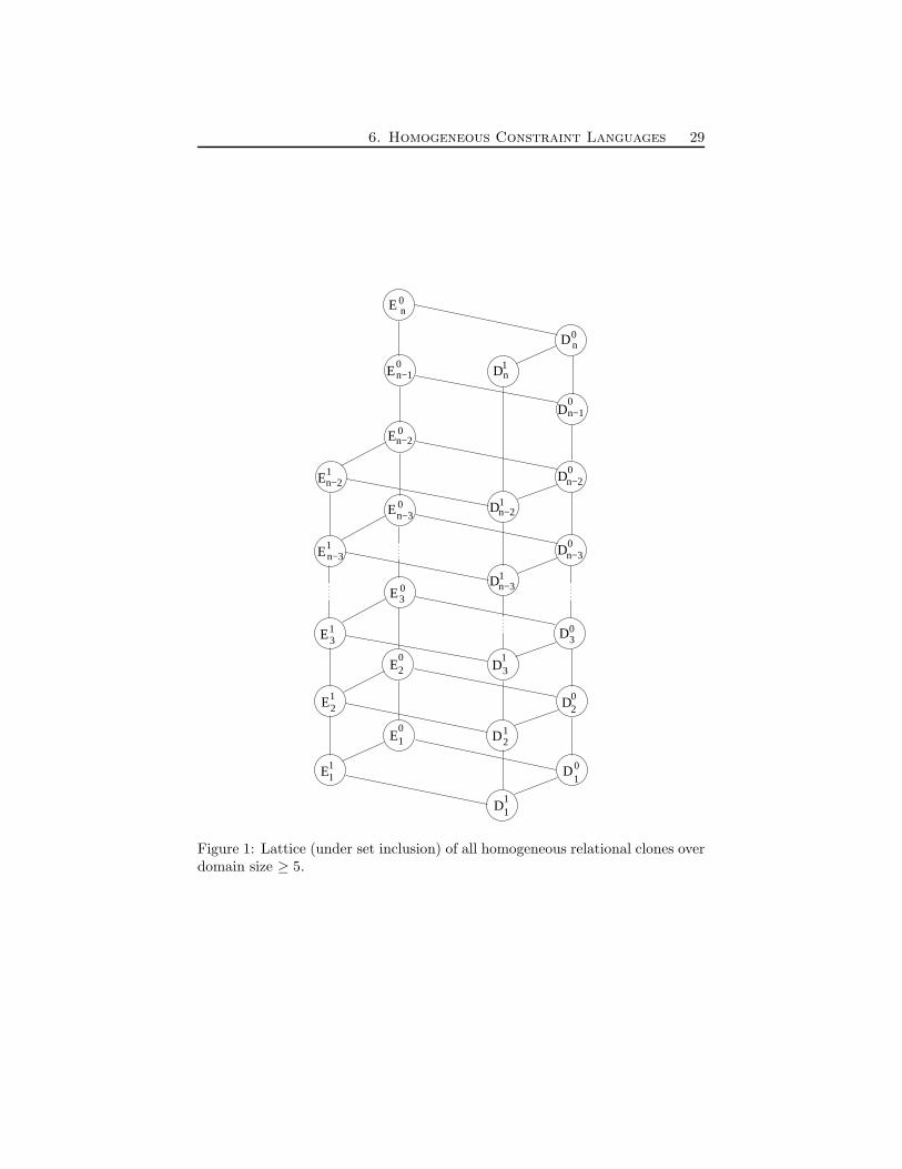
The lattice of all homogeneous relational clones on a domain D having n(≥ 5) elements is given in Figure 1. The lattice for the corresponding relationalclones over smaller domains (i.e., |D| ≤ 4) contains some exceptional relationalclones and are presented separately in Figures 2–4. Note that the correspond-ing lattices presented in [12] and [29] are the dual of ours, since they insteadconsider the inclusion structure among the corresponding clones of operations(but the two approaches are in fact equivalent as shown in [26] (Satz 3.1.2)).To understand the lattices we first need some definitions.
Throughout this section n denotes the size of the domain D, i.e., n = |D|.
Definition 6.2
• For a set D, the switching operation s on D is defined by
s(a, b, c) =
c if a = b,b if a = c,a otherwise.
• For a set D, the discriminator operation t on D is defined by
t(a, b, c) =
{c if a = b,a otherwise.
• For a set D, the dual discriminator operation d on D is defined by
d(a, b, c) =
{a if a = b,c otherwise.
• The k-ary near projection operation lk (3 ≤ k ≤ n) defined by
lk(a1, . . . , ak) =
{a1 if |{a1, . . . , ak}| < k,ak otherwise.
• The (n− 1)-ary operation rn defined by
rn(a1, . . . , an−1) =
{a1 if |{a1, . . . , an−1}| < n− 1,an otherwise.
In the second case we have {an} = D \ {a1, . . . , an−1}.
6. Homogeneous Constraint Languages 29
1
20
E
20
E01
D
D
D1
0
D0
E03
1
D12
E
E21
11
E13
D31
3
E
E
D
D
0
0
1
1
E
E
D
Dn−3
n−3
n−3
n−30
0
1
1
n−2
n−2
n−2
n−2
E
D
n−1
n−10
0
E
D0n
0n
D1n
Figure 1: Lattice (under set inclusion) of all homogeneous relational clones overdomain size ≥ 5.
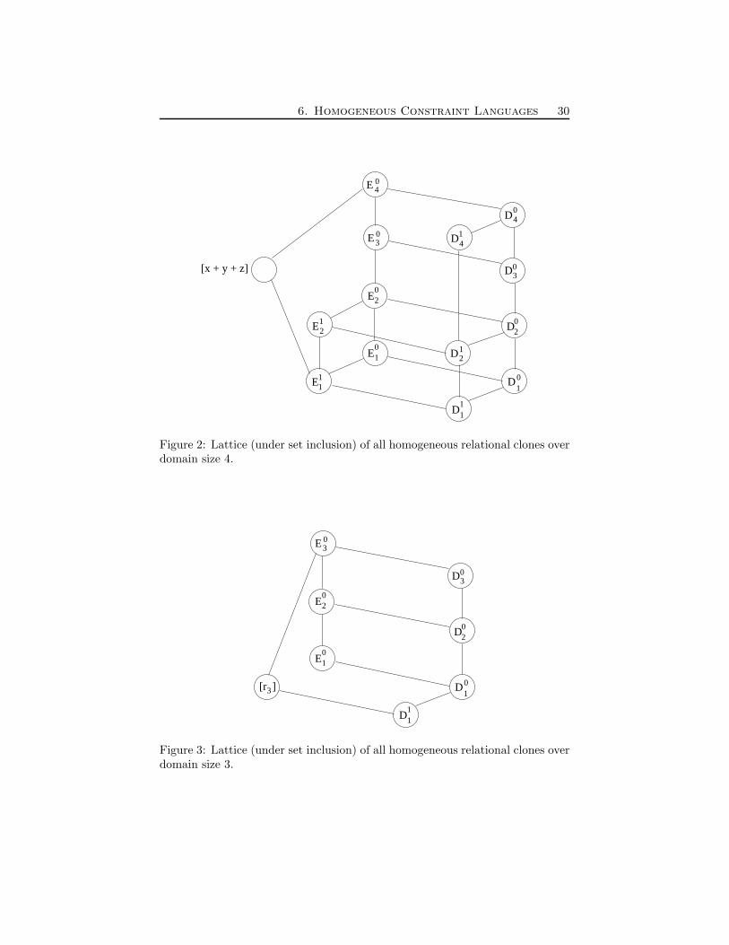
6. Homogeneous Constraint Languages 30
1
20
E
20
E01
D
D
D1
0
D0
E03
3
1
E40
04D
D12
D41
E
E21
11
[x + y + z]
Figure 2: Lattice (under set inclusion) of all homogeneous relational clones overdomain size 4.
1
20
E
20
E01
D
D
D1
0
D0
E03
3
[r ]3
1
Figure 3: Lattice (under set inclusion) of all homogeneous relational clones overdomain size 3.
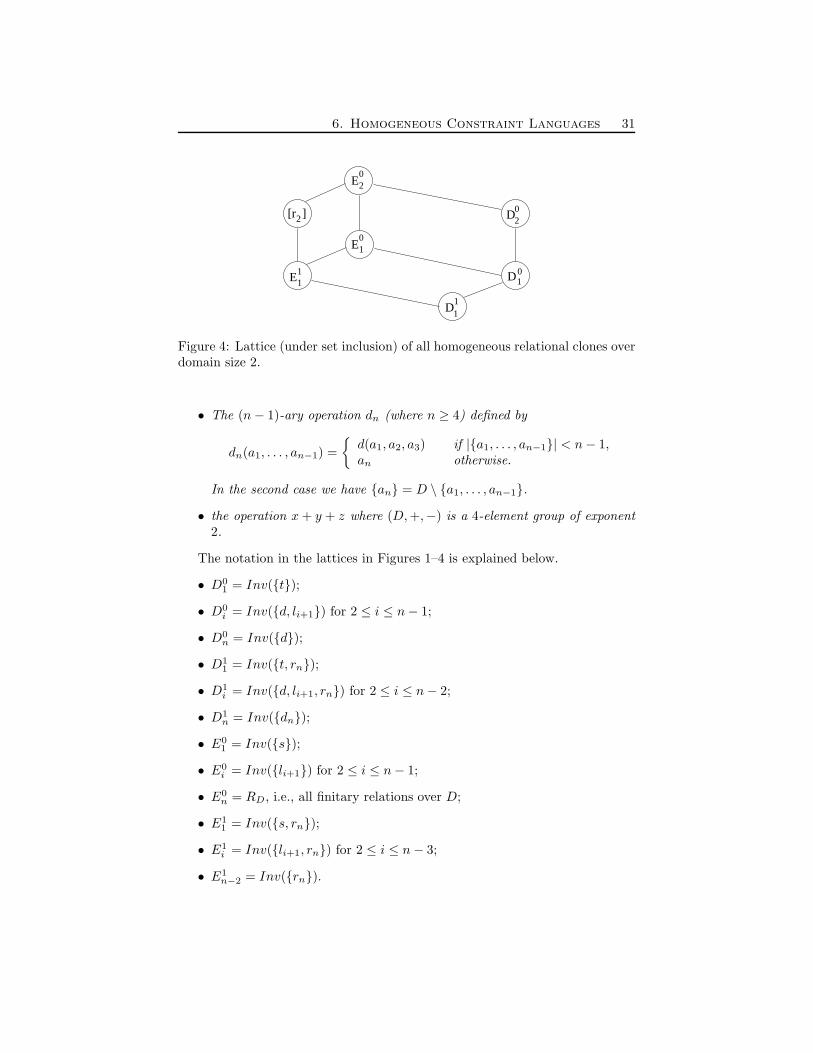
6. Homogeneous Constraint Languages 31
20
E
20
E01
D
D
D
E11
11
01
[r ]2
Figure 4: Lattice (under set inclusion) of all homogeneous relational clones overdomain size 2.
• The (n− 1)-ary operation dn (where n ≥ 4) defined by
dn(a1, . . . , an−1) =
{d(a1, a2, a3) if |{a1, . . . , an−1}| < n− 1,an otherwise.
In the second case we have {an} = D \ {a1, . . . , an−1}.
• the operation x+ y + z where (D,+,−) is a 4-element group of exponent2.
The notation in the lattices in Figures 1–4 is explained below.
• D01 = Inv({t});
• D0i = Inv({d, li+1}) for 2 ≤ i ≤ n− 1;
• D0n = Inv({d});
• D11 = Inv({t, rn});
• D1i = Inv({d, li+1, rn}) for 2 ≤ i ≤ n− 2;
• D1n = Inv({dn});
• E01 = Inv({s});
• E0i = Inv({li+1}) for 2 ≤ i ≤ n− 1;
• E0n = RD, i.e., all finitary relations over D;
• E11 = Inv({s, rn});
• E1i = Inv({li+1, rn}) for 2 ≤ i ≤ n− 3;
• E1n−2 = Inv({rn}).
6. Homogeneous Constraint Languages 32
We now state Dalmau’s classification for the complexity of Csp(Γ) for ho-mogeneous constraint languages Γ.
Theorem 6.3 ([12]) Let Γ be a homogeneous constraint language. Then Csp(Γ)is in P if Pol(Γ) contains the dual discriminator operation d, the switching op-eration s, or an affine operation. Otherwise, Csp(Γ) is NP-complete.
We have the following corollary to Dalmau’s classification.
Corollary 6.4 Let Γ be a homogeneous constraint language. Then W-MaxSol(Γ) is in poly-APX if Pol(Γ) contains the dual discriminator operation d,the switching operation s, or an affine operation. Otherwise, it is NP-hard tofind a feasible solution to W-Max Sol(Γ).
Proof. All dual discriminator operations, switching operations, and affine oper-ations are idempotent (i.e., f(x, x, x) = x for all x ∈ D). Hence, Γ is invariantunder a dual discriminator operation, switching operation, or an affine operationif and only if Γc = {Γ∪{{(d1)}, . . . , {(dn)}} is invariant under the correspondingoperation. Thus, it follows from Theorem 6.3 that Csp(Γc) is in P if Pol(Γ) con-tains the dual discriminator operation d, the switching operation s, or an affineoperation. This together with Lemma 3.2 gives us that W-Max Sol(Γ) is inpoly-APX if Pol(Γ) contains the dual discriminator operation d, the switchingoperation s, or an affine operation.
The NP-hardness part follows immediately from Dalmau’s classification inTheorem 6.3. ⊓⊔
We begin by investigating the approximability of W-Max Sol(Γ) for someparticular homogeneous constraint languages Γ.
Lemma 6.5 W-Max Sol(D0n) is in APX if 0 /∈ D and in poly-APX if
0 ∈ D.
Proof. Remember that D0n = Inv({d}). Hence, membership in poly-APX
follows directly from Corollary 6.4. It is known from Dalmau’s classification thatCsp(D0
n) is in P. Hence, by Proposition 3.1, it follows that W-Max Sol(D0n)
is in APX when 0 /∈ D. ⊓⊔
Lemma 6.6 W-Max Sol(D12) is APX-complete if 0 /∈ D and poly-APX-
complete if 0 ∈ D.
Proof. Choose any a, b ∈ D such that a < b. The relation r = {(a, a), (a, b), (b, a)}is in D1
i = Inv({d, li+1, rn}) for 2 ≤ i ≤ n− 2. Hence, by Lemmas 3.3 and 3.4,it follows that W-Max Sol(D1
2) is APX-hard if 0 /∈ D and poly-APX-hard if0 ∈ D. This together with Lemma 6.5 and fact that D1
i ⊆ D0n give us that W-
Max Sol(D12) is APX-complete if 0 /∈ D and poly-APX-complete if 0 ∈ D.
⊓⊔
Lemma 6.7 Finding a feasible solution to W-Max Sol(E12) is NP-hard.
6. Homogeneous Constraint Languages 33
Proof. Remember that E12 = Inv({l3, rn}) and, hence, it follows from Dalmau’s
classification in Theorem 6.3 that Csp(E12 ) is NP-complete. ⊓⊔
Lemma 6.8 W-Max Sol(D01) is in PO.
Proof. We will prove that D01 = Inv({t}) is equal to 〈ID〉, where ID is the class
of injective constraint languages from Definition 4.1. We begin by proving that〈ID〉 ⊆ Inv({t}). Consider an arbitrary relation R in ID and two arbitrarytuples a = (a1, a2) and b = (b1, b2) in R. From the definition of ID it followsthat a1 = b1 if and only if a2 = b2, i.e., two tuples in ID either disagree in allcoordinate positions or they are identical. Hence, given three arbitrary tuplesa, b, and c in R, t(a, b, c) = a when a 6= b and t(a, b, c) = c when a = b. Thus,ID ⊆ Inv({t}) and consequently 〈ID〉 ⊆ Inv({t}).
Now we will prove that if R is an arbitrary relation such that R /∈ 〈ID〉, then〈ID ∪ {R}〉 * Inv({t}). First note that 〈ID〉 contains all unary relations (so Rcannot be unary). Hence, it also contains all relations of the form A×B whereA and B are subsets (unary relations) of D, i.e., complete binary relations.Let S(x1, x2, . . . , xr) be an arbitrary constraint such that πxi,xi+1
(S) (for all0 < i < r) is either the complete constraint πxi
(S)×πxi+1(S) or a bijection from
πxi(S) to πxi+1
(S). Then, it is easy to realise that S (the underlying relationcorresponding to S(x1, x2, . . . , xr)) is in Inv({t}). Hence, R must have theproperty that for some 0 < i < r it hold that πxi,xi+1
(R(x1, x2, . . . , xt)) = R′,where R′ ⊂ πxi
(R)×πxi+1(R) and R′ is not a bijection from πxi
(R) to πxi+1(R).
A two-fan (as defined in [10]) is a binary relation of the form {(a × B)} ∪{(A × b)}, where a ∈ A and b ∈ B. Now, assume that R′ is a two-fan(but not a complete relation or a bijection). Then, there is a tuple (a′, b′) ∈A × B such that (a′, b′) /∈ R′. We have that {(a, b′), (a, b), (a′, b)} ⊆ R′ but(t(a, a, a′), t(b′, b, b)) = (a′, b′) /∈ R′ so R′ is not invariant under t.
It is proved in [10] (Lemma 6.1) that if R′ is a binary relation which is neithera two-fan, complete, nor a bijection; then 〈ID ∪ {R′}〉 contains at least one ofthe binary relations R′
1, R′2, or R
′3, where
• R′1 = {(a, a), (a, b), (b, c)},
• R′2 = {(a, a), (a, b), (b, c), (b, b)}, and
• R′3 = {(a, a), (a, b), (b, c), (b, b), (b, a)}.
Furthermore, a, b and c are all distinct. R′1 is not invariant under t since
(t(a, a, b), t(a, b, c)) = (b, a) /∈ R′1. The same example also shows that R′
2 is notinvariant under t (since (b, a) /∈ R′
2). To see that R′3 is not invariant under t,
observe that (t(b, b, a), t(c, b, a)) = (a, c) /∈ R′3.
Thus, we have indeed showed that if R is an arbitrary relation such thatR /∈ 〈ID〉, then 〈ID ∪ {R}〉 * Inv({t}). This together with the fact that〈ID〉 ⊆ Inv({t}) allow us to conclude that D0
1 = Inv({t}) = 〈ID〉. Hence, byLemma 4.2, we get the result that W-Max Sol(D0
1) is in PO. ⊓⊔
6. Homogeneous Constraint Languages 34
Lemma 6.9 W-Max Sol(Inv(E01)) is in APX.
Proof. Remember that E01 = Inv({s}). Dalmau give a polynomial-time algo-
rithm for Csp(Inv({s})) in [12] (he actually give a polynomial-time algorithmfor the more general class of para-primal problems). Dalmau’s algorithm ex-ploit in a clever way the internal structure of para-primal algebras to show thatany instance I of Csp(Inv({s})) can be split into independent subproblemsI1, . . . , Ij , such that
• the set of solutions is preserved (i.e., any solution to I is also a solutionto each of the independent subproblems, and any solution to all of theindependent subproblems is also a solution to I); and
• each Ii (1 ≤ i ≤ j) is either an instance of Csp(Inv({t})) or an instance ofCsp(Inv({a})), where t is the discriminator operation and a is an affineoperation.
Hence, to show that W-Max Sol(E01) is in APX, we first use Dalmau’s al-
gorithm to reduce the problem (in a solution preserving manner) to a set ofindependent W-Max Sol(Γ) problems where Γ is either invariant under anaffine operation or the discriminator operation. We know from Lemma 6.8 thatW-Max Sol(Γ) is in PO when Γ is invariant under the discriminator opera-tion, and from Theorem 5.13 we know that W-Max Sol(Γ) is in APX whenΓ is invariant under an affine operation. Since all the independent subprob-lems are in APX, we get that the original W-Max Sol(E0
1) problem is also inAPX. ⊓⊔
Lemma 6.10 W-Max Sol(Inv(E11)) is APX-complete.
Proof. Remember that E11 = Inv({s, rn}). Note that E1
1 ⊆ E01 so containment
in APX follows from Lemma 6.9.For the hardness part we begin by considering the general case where n =
|D| ≥ 4. Choose an arbitrary two-element subset {a, b} of D (without loss ofgenerality assume that a < b) and let (G,+,−) be the two element group onG = {a, b} defined by a+ a = a, a+ b = b+ a = b, and b+ b = a. Let Γ be theset of all relations expressible as the set of solutions to equations over (G,+,−).It is easy to realise that Γ is invariant under rn (since rn (n ≥ 4) acts as aprojection on {a, b}). Furthermore Γ is invariant under s since s(x, y, z) acts asthe affine operation x+ y+ z on {a, b}. It is proved in Lemma 5.8 that W-MaxSol Eqn(Zp, g) is APX-hard, and hence W-Max Sol(Γ) is APX-complete.For n = |D| = 3 there is no relational clone of the type E1
1 = Inv({s, rn}),hence the only case that remains to be dealt with is the case where n = |D| = 2.
Without loss of generality assume that D = {a, b} where a < b. Againconsider the group (G,+,−) on {a, b}. Let Γ = {R1, R2} where R1 is the (4-ary)relation on D which is the set of solutions to the equation x1+x2+x3+x4 = aand R2 is the (binary) relation representing the set of solutions to the equationy1 + y2 = b. Furthermore, let Γ0,1 = {R1, R2} denote the special case where
6. Homogeneous Constraint Languages 35
a = 0, b = 1 (i.e., D = {0, 1}). It has been proved in [22] (Lemma 6.9) that MaxSol(Γ0,1) is APX-complete. Let I be an instance of Max Sol(Γ0,1) containingk variables, then it is easy to realise that if I has a solution then opt(I) ≥ k/2(just note that the complement of any solution to I is also a solution to I). Wegive a L-reduction from Max Sol(Γ0,1) to Max Sol(Γa,b). Let F (I) be theinstance of Max Sol(Γa,b) where all occurrences of 0 has been replaced by aand all occurrences of 1 has been replaced by b. Since opt(I) ≥ k/2 we getthat opt(F (I)) ≤ bk ≤ 2b · opt(I) and hence β = 2b is a valid parameter inthe L-reduction. Let s be an arbitrary solution to F (I), then define G(F (I), s)to be the corresponding solution to I where a is replaced by 0 and b is replacedby 1. Then,
|m(G(F (I), s)) − opt(I)| ≤1
b− a|m(s)− opt(F (I))|
and thus γ = 1b−a
is a valid parameter in the L-reduction. This completes theAPX-hardness proof for Max Sol(Γa,b). Now, the unary operation r2 acts asthe non-identity permutation on {a, b} (i.e., r2(a) = b, and r2(b) = a) and henceboth R1 and R2 are invariant under r2. As we have already observed s acts asthe affine operation on {a, b} so R1 and R2 are also invariant under s. Hence,Γa,b ⊆ Inv({s, r2}) which concludes the proof. ⊓⊔
We have now proved all the results needed to give a complete classification forthe approximability of W-Max Sol(Γ) for all homogeneous relational clones Γover domains D of size at least 5. In order to complete the classification also fordomains of size 2, 3 and 4, we need to consider some exceptional homogeneousrelational clones that are not present for domains of sizes larger than or equalto 5. Over domains of size 4 we need to consider the homogeneous relationalclone Inv({x+ y+ z}) where + is the operation of a 4-element group (D,+,−)of exponent 2 (i.e., a 4-element group such that for all a ∈ D, a+ a = e wheree is the identity element in (D,+,−)).
Lemma 6.11 Let f(x, y, z) = x+ y+ z where (D,+,−) is a group of exponent2 then W-Max Sol(Inv({f})) is APX-complete.
Proof. The operation x+y+x is the affine operation on (D,+,−) (since −y = yin (D,+,−)) and hence if follows directly from Theorem 5.11 and Theorem 5.13that W-Max Sol(Inv({x+ y + z})) is APX-complete. ⊓⊔
Over 3-element domains it remains to classify the approximability of W-Max Sol(Inv({r3})), where r3 is the binary operation defined as follows
r(a1, a2) =
{a1 if a1 = a2,a3 where {a3} = D \ {a1, a2} otherwise.
Lemma 6.12 W-Max Sol(Inv({r3})) is APX-complete.
6. Homogeneous Constraint Languages 36
Proof. The operation r3(x, y) is actually an example of an operation of the typep+12 (x + y) (where + is the operation of an Abelian group of order |D| = p)
from Lemma 5.16. In our case p = 3 and r3(x, y) = 2x + 2y where + is theoperation of the Abelian group (D,+,−) isomorphic to Z3. Hence, it followsfrom Lemma 5.16 and Lemma 5.17 that W-Max Sol(Inv({r3})) is APX-complete. ⊓⊔
Over 3-element domains we also need to classify the approximability of W-Max Sol(E0
2) since hardness no longer follows from the hardness of W-MaxSol(E1
2) (there is no relational clone E12 over 3-element domains).
Lemma 6.13 It is NP-hard to find a feasible solution to W-Max Sol(E02).
Proof. Remember that E02 = Inv({l3}) and, hence, it follows from Dalmau’s
classification in Theorem 6.3 that Csp(E02 ) is NP-complete. ⊓⊔
Similarly, we also need to classify the approximability of W-Max Sol(D02)
since hardness no longer follows from the hardness of W-Max Sol(D12) (there
is no relational clone D12 over 3-element domains).
Lemma 6.14 W-Max Sol(D02) is APX-complete if 0 /∈ D and poly-APX-
complete if 0 ∈ D.
Proof. Remember that D02 = Inv({d, l3}) and, hence, it follows from the proof
of Lemma 6.6 that W-Max Sol(D02) is APX-complete if 0 /∈ D and poly-
APX-complete if 0 ∈ D. ⊓⊔
Over a two element domain {a, b} we need to classify the unary operationr2 which acts as the non-identity permutation (i.e., r2(a) = b and r2(b) = a).
Lemma 6.15 Finding a feasible solution to W-Max Sol(Inv({r2})) is NP-hard.
Proof. Let NAE be the following ternary relation on {a, b}: NAE = {a, b}3 \{(a, a, a), (b, b, b)}. The well-known NP-complete problem Not-All-Equal3-Sat [14] is exactly the problem of deciding whether there exists a feasiblesolution to Max Sol({NAE}) and thus finding a feasible solution to MaxSol({NAE}) is NP-hard. Now, remember that r2 is the non-identity per-mutation on {a, b} so it is easy to see that {NAE} ⊆ Inv({r2}). Thus, it isNP-hard to find a feasible solution to W-Max Sol(Inv({r2})). ⊓⊔
Finally we are in the position to present the complete classification for theapproximability of all homogeneous constraint languages.
Theorem 6.16 Let Γ be a homogeneous constraint language.
1. If 〈Γ〉 ∈ {Eij | i ∈ {0, 1}, j ≥ 2} or 〈Γ〉 = Inv({r2}) then it is NP-hard to
find a feasible solution to W-Max Sol(Γ);
2. else if, 0 ∈ D and 〈Γ〉 ∈ {Dij | i ∈ {0, 1}, j ≥ 2} then W-Max Sol(Γ) is
poly-APX-complete;
7. Conclusions 37
3. else if,
〈Γ〉 ∈ {E11 , E
01 , Inv({x+ y + z}), Inv({r3})} or
〈Γ〉 ∈ {Dij | i ∈ {0, 1}, j ≥ 2} and 0 /∈ D,
then W-Max Sol(Γ) is APX-complete;
4. otherwise, 〈Γ〉 ∈ {D11, D
01} and W-Max Sol(Γ) is in PO.
Proof. We know from Theorem 2.9 that it is sufficient to consider constraintlanguages that are relational clones.
1. Follows from the fact that E12 ⊆ E1
j and E02 ⊆ E0
j (n ≥ j ≥ 2) togetherwith Lemmas 6.7, 6, and 6.15.
2. Follows from the fact that D12 ⊆ D1
j ⊆ D0n and D0
2 ⊆ D0j ⊆ D0
n (n ≥ j ≥2), together with Lemmas 6.5, 6.6, and 6.14.
3. Follows from the fact that D12 ⊆ D1
j ⊆ D0n, D
02 ⊆ D0
j ⊆ D0n (n ≥ j ≥ 2),
and E11 ⊆ E0
1 together with Lemmas 6.5, 6.6, 6.9, 6.10, 6.11, 6.12, and6.14.
4. Follows from the fact that D11 ⊆ D0
1 together with Lemma 6.8. ⊓⊔
As a direct consequence of the preceding theorem we get that the class ofinjective relations from Definition 4.1 is a maximal tractable class for W-MaxSol(Γ). That is, if we add a single relation which is not an injective relation tothe class of all injective relations, then the problem is no longer in PO (unlessP = NP).
Corollary 6.17 Let ΓDI be the class of injective relations from Definition 4.1
and r an arbitrary relation which is not in ΓDI . Then, W-Max Sol(ΓD
I ∪ {r})is not in PO (unless P = NP).
Proof. We know from the proof of Lemma 6.8 that D01 = Inv({t}) = ΓD
I =〈ID〉. It follows from the lattices of homogeneous relational clones that eitherE0
1 ⊆ D01 ∪ {r} or D0
2 ⊆ D01 ∪ {r}. We know from Lemma 6.10 and Lemma 6.6
that both W-Max Sol(E01) and W-Max Sol(D0
2) are APX-hard. Thus, W-Max Sol(D0
1 ∪ {r}) is APX-hard and it follows that W-Max Sol(ΓDI ∪ {r})
is not in PO (unless P = NP). ⊓⊔
7 Conclusions
We view this paper as a first step towards a better understanding of the approx-imability of non-Boolean W-Max Sol. The ultimate long-term goal for thisresearch is, of course, to completely classify the approximability for all finiteconstraint languages. However, we expect this to be a hard nut to crack since
REFERENCES 38
not even a complete classification for the corresponding decision problem Cspis known. A more manageable task would be to completely classify W-MaxSol for constraint languages over small domains (say, of size 3 or 4). For size3, this has already been accomplished for Csp and Max Csp.
It is interesting to note that the applicability of the algebraic approach toW-Max Sol demonstrated in this paper also holds for the corresponding min-imisation problem W-Min Sol, that is, Theorem 2.9 still holds. The questionwhether the algebraic approach can shed some new light on the intriguing ap-proximability of minimisation problems (as manifested, e.g., in [22]) is an in-teresting open question. It is known from [22] that the approximability of theweighted and unweighted versions of (W)-Max Sol coincide for all Booleanconstraint languages. We remark that the same result holds for all constraintlanguages considered in this paper (i.e., maximal constraint languages and con-straint languages containing all permutation relations). This can be readilyverified by observing that the AP -reduction from W-Max Sol to Max Sol inthe proof of Lemma 3.11 in [22] easily generalises to arbitrary finite domains andthat our tractability proofs are given for the weighted version of the problem.As AP -reductions do not, in general, preserve membership in PO it still anopen problem if for every constraint language Γ tractability (i.e., membershipin PO) of Max Sol(Γ) implies tractability of W-Max Sol(Γ). The results inthis paper also raises some minor questions such as the following: Is the class ofgeneralised max-closed constraints a maximal tractable class for W-Max Sol?
References
[1] P. Alimonti and V. Kann. Some APX-completeness results for cubic graphs.Theor. Comp. Sci., 237:123–134, 2000.
[2] O. Angelsmark. Constructing Algorithms for Constraint Satisfaction Prob-lems and Related Problems – Methods and Applications. PhD thesis,Linkopings universitet, 2005.
[3] O. Angelsmark and J. Thapper. A microstructure based approach to con-straint satisfaction optimisation problems. In Proceedings of the 18th In-ternational FLAIRS Conference (FLAIRS 2005), pages 155–160, 2005.
[4] G. Ausiello, P. Crescenzi, G. Gambosi, V. Kann, A. Marchetti Spaccamela,and M. Protasi. Complexity and approximation: Combinatorial optimiza-tion problems and their approximability properties. Springer, 1999.
[5] A. Bulatov. A dichotomy theorem for constraints on a three-element set.In Proceedings of the 43rd IEEE Symposium on Foundations of ComputerScience (FOCS 2002), pages 649–658, 2002.
[6] A. Bulatov. A graph of a relational structure and constraint satisfactionproblems. In Proceedings of the 19th IEEE Symposium on Logic in Com-puter Science (LICS 2004), pages 448–457, 2004.
REFERENCES 39
[7] A. Bulatov, P. Jeavons, and A. Krokhin. Classifying the complexity ofconstraints using finite algebras. SIAM J. Comput., 34(3):720–742, 2005.
[8] A. Bulatov, A. Krokhin, and P. Jeavons. The complexity of maximal con-straint languages. In Proceedings of the 33rd ACM Symposium on Theoryof Computing (STOC 2001), pages 667–674, 2001.
[9] D.A. Cohen. Tractable decision for a constraint language implies tractablesearch. Constraints, 9(3):219–229, 2004.
[10] M. Cooper, D.A. Cohen, and P. Jeavons. Characterizing tractable con-straints. Artificial Intelligence, 65(2):347–361, 1994.
[11] N. Creignou, S. Khanna, and M. Sudan. Complexity classifications ofBoolean constraint satisfaction problems. SIAM, Philadelphia, 2001.
[12] V. Dalmau. A new tractable class of constraint satisfaction problems. An-nals of Mathematics and Artificial Intelligence, 44(1–2):61–85, 2005.
[13] T. Feder and M.Y. Vardi. The computational structure of monotonemonadic snp and constraint satisfaction: A study through datalog andgroup theory. SIAM J. Comput., 28(1):57–104, 1999.
[14] M.R. Garey and D.S. Johnson. Computers and Intractability: A Guide tothe Theory of NP-Completeness. Freeman, San Francisco, 1979.
[15] D.S. Hochbaum and J. Naor. Simple and fast algorithms for linear andinteger programs with two variables per inequality. SIAM J. Comput.,23(6):1179–1192, 1994.
[16] C.M. Hoffmann. Group-Theoretic Algorithms and Graph Isomorphism, vol-ume 136 of Lecture Notes in Computer Science. Springer, 1982.
[17] P. Janssen, P. Jegou, B. Nouguier, and M.C. Vilarem. A filtering process forgeneral constraint satisfaction problems: achieving pair-wise consistencyusing an associated binary representation. In Proceedings of the IEEEWorkshop on Tools for Artificial Intelligence, pages 420–427, 1989.
[18] P. Jeavons. On the algebraic structure of combinatorial problems. Theo-retical Computer Science, (200):185–204, 1998.
[19] P. Jeavons, D. Cohen, and M. Gyssens. Closure properties of constraints.Journal of the ACM, 44:527–548, 1997.
[20] P. Jonsson. Near-optimal nonapproximability results for some NPO PB-complete problems. Information Processing Letters, 68(5):249–253, 1998.
[21] P. Jonsson, M. Klasson, and A. Krokhin. The approximability of three-valued Max CSP. SIAM J. Comput. (To appear), 2005.
REFERENCES 40
[22] S. Khanna, M. Sudan, L. Trevisan, and D.P. Williamson. The approxima-bility of constraint satisfaction problems. SIAM J. Comput., 30(6):1863–1920, 2000.
[23] F. Kuivinen. Tight approximability results for the maximum solution equa-tion problem over Zp. In Proceedings of the 30th International Symposiumon Mathematical Foundations of Computer Science (MFCS 2005), pages628–639, 2005.
[24] S.S. Marchenkov. Homogeneous algebras. Problemy Kibernetiki, 39:85–106,1982.
[25] E. Marczewski. Homogeneous algebras and homogeneous operations. Fund.Math., 56:81–103, 1964.
[26] R. Poschel and L. Kaluznin. Funktionen- und Relationenalgebren. DVW,Berlin, 1979.
[27] A. Schrijver. Theory of linear and integer programming. John Wiley &Sons, Inc., New York, NY, USA, 1986.
[28] B. Szczepara. Minimal clones generated by groupoids. PhD thesis, Univer-site de Montreal, 1996.
[29] A. Szendrei. Clones in Universal Algebra, volume 99 of Seminaries deMathematiques Supereiores. University of Montreal, 1986.
[30] G.J. Woeginger. An efficient algorithm for a class of constraint satisfactionproblems. Operations Research Letters, 30(1):9–16, 2002.