h-. 1~~==. ;, ‘- - federation of american scientists · 2016-10-21 · .4, ..%. ).x,nz--r- ... ....
TRANSCRIPT

~=----- -- —— ..—— .....- . ? ,.. -=. .. ;, 9
1~~== --”...,,:...,.,H-.
).
.- --: —.—------- .-, .,+-—---T — ..7. i.. -—
.<1,
., Q.*. ~ . ! ,... .>,. _-&--
. . . . . ..—
-4.’2---:. .-w;, <~ %,,.:”.-.?- = -. :.-u . . /’=”’- -“ - ‘-._:_..~~.:{~_.; +;+-4*~~2.&2z7.:&, .. . *. .. . . .. C;:..-,..,.:.-.. . . —-. ..— --. — ,., . . . . ~. -—.. . . >.. . . .
‘“LA-.9445-PN~ ,- ~ “,:c, !. <..-i” . .. . . .-.S.L+~. ,ry-.... L ~--f-y. .... .---.....*-. . ..T++w=- .Twffw~FR&-d”r-~.s%~4i+z.wwJ.-=;r-.-”-- -:.”~.-.-:-- ----- Lb---~--.-_.a . A -— —--.—------- ......... ....—...—,~. ,+.—... .—---- -------—.----—-----—-------.-——-.--. ——...—<.,.*-. . -,‘-

-*. . . . . .. ., .-..:.- . .
!.. . .
.. . .. ...... .. .. . . . ..b ,., ,J. ... . . .
.,
.,. . .
.
. . ,., ,
. .
.
. .-. . .. . . . . ------ . .. T._ . ..&_.
<..
.-..
,,-.. .;-. .
.:.“. . ,,
,. .,-. .
.,.1
.*.-;.
,,,.:.-,
‘I’& report w~s prepared ‘by Kathy Derouin; “b”is Schneider, and Mary Lou
@gher, Group ‘H-8:’ “ . ._ - “‘_
,’: ,.
-. .h.
,,
., ,~,. ,.,
,., -.,- ..,, -
,.
.
.,L-
,,. . . . . .. . ..--%-m!-+=-,e.m.m .4, . .%. . . . ) .X,nz-- AJ- -,,,%. ,r- —-. .%-.-...*Tlda report was prepared aa an account of wnrk qronaored y an agency of the United States Government.
Neither the United !lma Covmvncnt nor anY agerky thereof, nor any of their” employees, makca artywartznty, express or implied, or assumesany ie# liability or responsibility for the accuracy, compktencaa,
.- .,., :,:. .& wNU+ Qfw.inf&@Qm appmtm prodfid, Or pr~ ~~d, w rcw=nta that fi U= ~~d,.. . ,W. +4 ,q irlf~ privately owned ri@~_Referencca herein to any
TK c-ercial product, prows, or
~.. .% ~ ~,l+2~~~W@e;[ti+=~!~. Wafi{c!~:~r ~i--~~ h~~—~~maiuie or iqplYita
,.. - . ., m,-.. .--- .
omement, reEomme%EAon, or LGktg ky & ‘fftii&lTiiteaT%wrunent or any S&”~cytAereof. The---- -..., ...
. . .; ’’-:. ..-— . .,. vbk”~j%%ii~i~i=i expreaadk%ti-do notn+y @&”rcfit =of die Uiiited’ -
- -. —.. ., .,.... . ..-.—
&aM Cownment or any agency’thereof.. . . . . .... . . ...”. ,- .,, ., _..
..-. ,., .”..” . ...--! ,. +,. . . - ~,. —----- . ..” — .Z..fi . . . . . ,.
r. -.
“.-“-...-A? .
., ..-
.-.%

LA-9445 -PNTX-D
Issued: December 1982
Supplementary Documentation for anEnvironmental Impact Statement
Regarding the Pantex Plant
Dispersion Analysis forPostulated Accidents
J.M. DewartB. M. BowenJ.C. Elder
~~~ ~kl~~~ LosAlamos,NewMexico87545Los Alamos National Laboratory


CONTENTS
ABSTRACT 1
I. INTRODUCTION 1
II. THE DIFOUT MODELA. BackgroundB. Dispersion and Deposition Assumptionsc. Source Characterization
1. Cloud Shape2. Aerosol Parameters
D. MeteorologyE. Model Verification
III. DATA BASE FOR DIFOUT MODEL CALCULATIONS
A. Cloud Parameters1. Cloud Height2. Cloud Diameter3. Plutonium Distribution with Height4. Aerosol Size Distribution
B. Meteorological Data1. STAR Data2. Meteorological Data Used as DIFOUT Kbdel Input3. Site Data
IV. RESULTS AND DISCUSSION
v. SUMMARY
ACKNOWLEDGMENTS
REFERENCES
APPENDICES
A. CALCULATION RESULTS
B. STABILITY - WIND ROSE (STAR) DATA
c. DIFOUT MODEL VERIFICATION STUDY
23445555
6
668101011111318
18
25
25
26
28
44
53
v

FIGURES
1.
2.3.4.5.
6.c-1.
c-2.
c-3.c-4.c-5.C-6.c-7.C-8.c-9 .
Wind rose for Amarillo, Texas, 1955-1964Wind rose for Burlington, Iowa, 1967-1971Wind rose for the Hanford Site, Washington, 1973-1975Location of the Pantex Plant and surrounding communitiesLocation of the Iowa Army Ammunition Plant and surroundingcommunitiesLocation of the Hanford Site and surrounding communitiesOutline of debris cloud (Double Tracks at 105 s afterdetonation; Clean S1ate 2, 120 s)Distribution of plutoniun with height for Double Tracks andClean Slate 2 testsAerosol size distribution for Roller Coaster experimentsVariation of median particle diameter with distancePeakPeakPeakPeakPeak
C-10. Peak
I.II.
III.IV.v.VI.VII.VIII.IX.x.XI.XII.
XIII.
XIV.
xv.
vi
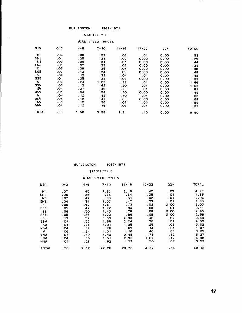
airborne dosage - Double Tracksdeposited dosage - Double Tracksairborne dosage - Clean Slate 1deposited dosage - Clean Slate 1airborne dosage - Clean S1ate 2deposition - Clean S1ate 2
TABLES
ROLLER COASTER TEST SHOTSPOSTULATED ACCIDENTS: HIGH EXPLOSIVES DETONATED ANDPLUTONIUM RELEASEDROLLER COASTER DATA FOR POSTULATED ACCIDENTSCLOUD DIAMETERS (m) FCR POSTULATED ACCIDENTSCLOUD DIAMETERS (m) FOR ACCIDENTS J, K, S, and TPLUTONILFI DISTRIBUTION WITH HEIGHTAEROSOL SIZE DISTRIBUTION PARAMETERSWIND DIRECTIONS F(R DISPERSION CASESMETEOROLOGICAL DATA FOR UNFAVORABLE AND MEDIAN DISPERSION CASESWIND SPEED EXPONENT AND TURBULENCE INTENSITY VALUESMETEOROLOGICAL DATA FOR TORNADO ACCIDENTDISTANCES TO SITE BOUNDARY, NEAREST RESIDENCE, ANDMAJOR POPULATION CENTERHIGHEST OFFSITE INTEGRATED AIR CONCENTRATION AND GROUNDDEPOSITION FOR PANTEX PLANT ACCIDENTSHIGHEST OFFSITE INTEGRATED AIR CONCENTRATION AND GROUNDDEPOSITION FOR IAAP ACCIDENTSHIGHEST OFFSITE INTEGRATED AIR CONCENTRATION AND GROUNDDEPOSITION FOR HANFORD SITE ACCIDENTS
1213141920
2156
58
5961626263646667
37
889
10111517171822
23
24
24

SUPPLEMENTARY DOCUMENTATION FOR AN ENVIRONMENTAL IMPACT STATEMENTREGARDING THE PANTEX PLANT:
DISPERSION ANALYSIS FOR POSTULATED ACCIDENTS
by
J. M. Dewart, B. M. Bowen, and J. C. Elder
ABSTRACT
This report documents work performed in support of preparation of anEnvironmental Impact Statement (EIS) regarding the Department of Energy(DOE) Pantex Plant near Amarillo, Texas. The report covers the calculationof atmospheric dispersion and deposition of plutonium following postulatednonnuclear detonations of nuclear weapons. Downwind total integrated airconcentrations and ground deposition values for each postulated accident arepresented. The model used to perform these calculations is the DIFOUTmodel, developed at Sandia National Laboratories in conjunction withOperation Roller Coaster, a field experiment involving sampling andmeasurements of nuclear material dispersed by four detonations. The DIFOUTmodel is described along with the detonation cloud sizes, aerosolparameters, and meteorological data used as input data. A verificationstudy of the DIFOUT model has also been performed;in Appendix C.
the results are presented
I. INTRODUCTION
This report documents work performed in support of preparation of anEnvironmental Impact Statement (EIS) regarding the Department of Energy (DOE)Pantex Plant near Amarillo, Texas. The EIS addresses continuing nuclearweapons operations at Pantex and the construction of additional facilities tohouse those operations. The EIS was prepared in accordance with currentregulations under the National Environmental Policy Act. Regulations of the
- ~ilMmiiMiiilllllllllllll~:------ .39338003080636
1

Council on Environmental Quality (40 CFR 1500) require agencies to prepareconcise EISS with less than 300 pages for complex projects. This report wasprepared by the Los Alamos National Laboratory to document details of workperformed and supplementary information considered during preparation of theDraft EIS.
The Pantex Plant is a nuclear weapons assembly/disassembly facilitylocated 25 km to the east-northeast of Amarillo, Texas. The EIS covers theexisting Pantex Plant facilities; new facilities and/or upgrading facilitiesat the Pantex Plant; moving a portion of the Pantex facilities to the IowaArmy Ammunition Plant (IAAP) at Burlington, Iowa; and building a new plant atthe IAAP or on the Hanford Site in eastern Washington.
As part of the Pantex EIS, several accidents involving the detonation ofhigh explosives in the presence of plutonium have been postulated (Chamberlain1982). Several initiating events have been assumed to cause a detonation ofhigh explosives: these include a tornado, an aircraft crash, and anoperational accident (such as dropping high explosives during assembly/disassembly). A complete description of the postulated accidents is bynecessity classified and is presented in Chamberlain (1982). The accidentshave been assigned letter designations (A, B, C, etc.) (Chamberlain 1982) andare presented in this manner for this report.
To estimate the health consequences and cleanup costs from theseaccidents at each of the three sites considered in the EIS, atmosphericdispersion and deposition modeling have been performed. This report presentsthe results of the dispersion and deposition calculations, which are used byElder (1982B) and Wenzel (1982B, 1982E) to assess these health and monetaryimpacts. A description of the DIFOUT model, used to perform the calcula-tions, and the data used as input to the model are also presented.
A verification study was performed on the DIFOUT model to assess itspredictive capabilities for this study. The model verification is presentedin Appendix C of this report, and a summary of specific verification resultsthat were employed in this study is presented in Section 11.E.
II. THE DIFOUT MODEL
This section of the report focuses on aspects of the DIFOUT model mostimportant to this study: the background of the model, dispersion anddeposition assumptions, source characterization, and the requiredmeteorological data. The actual data used in the DIFOUT model calculationsare presented in Sec. 111. For a complete description of all DIFOUT modelfeatures, including the model equations, the reader is referred to Luna(1969).
2
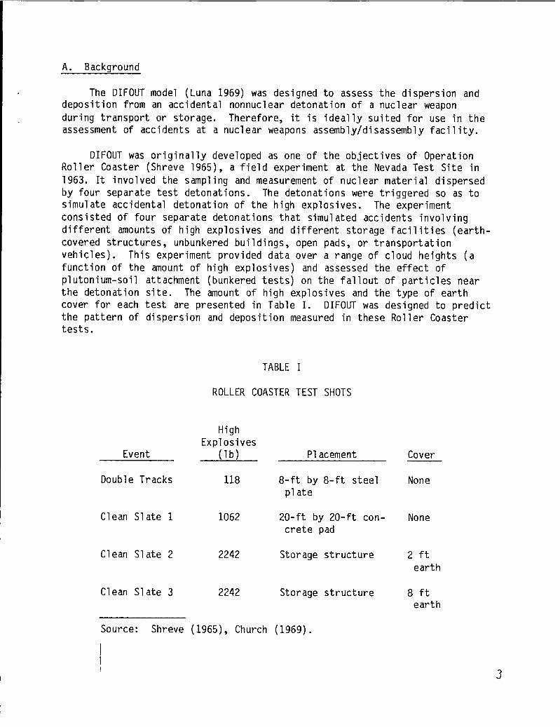
A. Background
The DIFOUT model (Luna 1969) was designed to assess the dispersion anddeposition from an accidental nonnuclear detonation of a nuclear weaponduring transport or storage. Therefore, it is ideally suited for use in theassessment of accidents at a nuclear weapons assembly/disassembly facility.
DIFOUT was originally developed as one of the objectives of OperationRoller Coaster (Shreve 1965), a field experiment at the Nevada Test Site in1963. It involved the sampling and measurement of nuclear material dispersedby four separate test detonations. The detonations were triggered so as tosimulate accidental detonation of the high explosives. The experimentconsisted of four separate detonations that simulated accidents involvingdifferent amounts of high explosives and different storage facilities (earth-covered structures, unbunkered buildings, open pads, or transportationvehicles). This experiment provided data over a range of cloud heights (afunction of the amount of high explosives) and assessed the effect ofplutonium-soil attachment (bunkered tests) on the fallout of particles nearthe detonation site. The amount of high explosives and the type of earthcover for each test are presented in Table I. DIFOUT was designed to predictthe pattern of dispersion and deposition measured in these Roller Coastertests.
TABLE I
ROLLER COASTER TEST SHOTS
HighExplosives
Event (lb)
Double Tracks 118
Clean Slate 1 1062
Clean S
Clean S
ate 2 2242
ate 3 2242
Source: Shreve (1965), Church
1
Placement
8-ft by 8-ft steelplate
20-ft by 20-ft con-crete pad
Storage structure
Storage structure
(1969).
None
None
2 ftearth
8 ftearth
3I

The verification study performed with the DIFOUT model (Appendix C)indicates that DIFOUT is an acceptable model for use in this study.
B. Dispersion and Deposition Assumptions
DIFOUT is a tilting plume Gaussian dispersion model. It includes aerosoldepletion through particle fallout and the effects on dispersion of windspeed and direction variation with height. The aerosol cloud produced by thedetonation is divided into several horizontal cylindrical layers, eachcontaining a specified amount of the total aerosol of the cloud. The aerosolis dispersed from a vertical line source in each layer; the downwindintegrated air concentrations (ug-s/m3) and ground deposition (ug/m2) are asum of the contributions from the line source in each layer.
The DIFOUT model allows two alternative methods for determiningdispersion coefficients required in the Gaussian equation: Sutton’s powerlaw relation or the turbulence intensity formulation of Smith and Hay (Slade1968). The Smith and Hay method, which was chosen for this study, calculateshorizontal and vertical dispersion coefficients (u , az) as a function ofdownwind distance and turbulence intensities. iTur ulence intensity values(!y, Iz) are a measure of the horizontal and vertical fluctuatwind, proportional to the standard deviation of the horizontalwind velocities divided by the horizontal wind speed.
The initial size of the cloud is also taken into accounthorizontal dispersion coefficients. A virtual source distance
ons of theand vertical
n calculatingis added to
all downwind ranges such that, at the initial location of the cloud, cryhasa finite value proportional to the cloud diameter.
Deposition values are calculated in DIFOUT as the product of theintegrated air concentration and the deposition velocity. For a givenparticle size, the deposition velocity is a function of the gravitationalfall velocity, wind speed, turbulence intensity, and reflection coefficient.The reflection coefficient varies from zero to one for a completelydepositing aerosol to a nondepositing aerosol. It is calculated as afunction of the particle fall velocity, wind speed, downwind distance, andinitial height of the particle.
c. Source Characterization
The DIFOUT model requires, as input data, a detailed description of theinitial stabilized detonation cloud (that is, no further cloud rise due tothe initial detonation). The cloud shape, including height and diameter, andaerosol characteristics, including mass distribution with height and sizedistribution, must be specified.
4
1. Cloud Shape. For each detonation cloud modeled with DIFOUT, thecloud=ight must first be determined. This cloud height is then divided into10 layers of equal thickness; the height of each layer is input data for themodel. The diameter of each layer must also be specified.
2. Aerosol Parameters. The DIFOUT model provides a method forcompletely describing the aerosol as it exists in the detonation cloud.DIFOUT input parameters include the distribution of aerosol mass with heightand the aerosol size distribution. For each of the 10 layers of the cloud,the fraction of the total aerosol and the aerosol size distribution must bespecified. The model also allows the user to select the size range of aerosolto be considered when summing the different vertical line source contri-butions to the integrated air concentrations and the ground deposition.
The aerosol size distribution may vary from layer to layer or beconstant over as many layers as desired. The distributions may be specifiedin two different manners for input to the model. The manual method requiresthat the specific particle diameters and the percentage of aerosol of eachsize be entered as input data for each layer. In the alternate method used inthis study, the distribution is approximated by line segments from a logprobability plot. This method requires the geometric standard deviation,activity (mass) median aerodynamic diameter (amad), and the upper and lowerlimits of particle diameter for each line segment; the model computes themass in each size fraction.
D. Meteorology
The meteorological parameters required by DIFOUT for dispersion of thedetonation cloud are wind speed, wind direction, and turbulence intensity.All these parameters may be varied with height so that the cloud can bemodeled realistically.
E. Model Verification
Based on the results of the model verification (Appendix C), thefollowing assumptions have been applied to the modeling of postulatedaccidents for this study.
1. The respirable fraction of plutonium aerosol was not modeled usingDIFOUT. Air concentrations of the total aerosol were calculated, and therespirable fraction was assumed to be 20% of these values.
2. Data from the Roller Coaster, Double Tracks, and Clean Slate 2 testswere determined to be appropriate for the description of the initialdetonation clouds. These data include the distribution of aerosol withheight, aerosol size distribution, and cloud diameter. Data from the Clean
5

Slate 1 test were judged to be inappropriate for describing the initialdetonation clouds.
III. DATA BASE FOR DIFOUl MODEL CALCULATIONS
The actual data used as input to the model for the calculation ofdispersion and deposition of plutonium from each of the postulated accidents(Table II) are presented in this section. These data include the parametersthat characterize the initial detonation cloud and the meteorologicalconditions that were used for calculating downwind air concentrations andground deposition.
A. Cloud Parameters
Measurements from the Roller Coaster test shots provide the bestavailable data for the initial stabilized cloud description required for thisstudy. These data include aerosol size distribution, distribution ofplutonium with height, and cloud diameter. Some Roller Coaster data havebeen used directly in this study. Other data were modified because ofdifferences between the postulated accidents and the Roller Coaster testshots . Each of the accidents postulated (Chamberlain 1982) has been comparedto the Roller Coaster test detonations. Data from the test most closelyresembling the accidents considered in this study were used in the DIFOUTmodel . Roller Coaster test data were applied to each accident as shown inTable III.
For most of the accidents, the Double Tracks test (an unbunkered test)was the appropriate choice. Clean Slate 2 data (a bunkered test) were chosenfor the other accidents. Clean Slate 1 data were not selected even thoughthe test involved more comparable amounts of high explosives for some of theaccidents than did Double Tracks. (The Clean S1ate 1 distribution ofplutonium with height was not considered representative.) Also, the DIFOUTmodel verification study (Appendix C) indicated inconsistencies betweenmodeling results and measurements for Clean Slate 1.
Cloud parameters specific to clouds resulting from all accidentsdiscussed in the following sections.
1. Cloud Height. For each postulated accident, the height of thetop was calculated as a function of the amount of high explosives invo’the detonation (Church 1969):
H = 76 (HE)O”ZS , (1)
,re
cloudved in
where H is the height of the cloud in meters and HE is the amount of highexplosives in pounds. When the cloud reaches this height, no further rise
6

TABLE II
POSTULATED ACCIDENTS: HIGH EXPLOSIVES DETONATEDAND PLUTONIUM RELEASED
Pantex Plant
High PlutoniumExplosives*** Released
(lb) (kg)
IAAP
LM+
:PQRs
Hanford Site
T
50010001000300183183114
2000420
k:
183
11:114300
200042019.6
1::1002512128
1;:0.0560.625
120.46088
25
1::0.625
19.6 0.625
CloudHeight(m)
35942742731628028024850834467**
135**
280119248248316508344135**
135**
*Dispersion and deposition values will not be calculated for theseaccidents. Considering the amount of high explosives and plutonium, theimpact of these accidents will be no greater than the impact fromaccidents E or F (Pantex) or L (IAAP).
**The cloud height has been calculated based upon one-half of the highexplosive involved because the cloud was released through two separatepoints (Chamberlain 1982).
***These are the effective anounts of high explosives detonated, representingthe amount of energy available for the initial cloud rise (Chamberlain1982) .
‘Dispersion and deposition values will not be calculated for this accident.Considering the amount of high explosives and plutonium, the impact ofthis accident will be no areater than was accident S.+–-— .—-.. .—.
7

TABLE 111
ROLLER COASTER DATA FOR POSTULATED ACCIDENTS
Applicable RollerAccident* Coaster Test Shot
H, I, Q, R Clean Slate 2
J, K, S, T Modified Double Tracks
A, B, C, D, E, F, G, L, Double TracksM, N, O, P
*Independent’of location and initiating event (tornado, aircraft crash,etc.).
Cloud Top
Layer 10*Layer 9Layer 8Layer 7Layer 6Layer 5Layer 4Layer 3Layer 2Layer 1Surface
TABLE
CLOUD DIAMETERS (m) FOR
Accidents A-G, J-P,
67787134911281157191121
—
IV
POSTULATED ACCIDENTS
S, T Accidents H, I, Q, R
122189250209818168135162155
*Each layer is of equal thickness.
occurs as a result of the initial detonation. The cloud heights for each ofthe postulated accidents are presented in Table II.
2. Cloud Diameter. For each accident analyzed, cloud diameters eitherwere taken directly from Double Tracks or Clean Slate 2 measurements (TableIV) or were a modification of the Double Tracks measurements. Using the
8

Double Tracks diameters is a conservative assumption: each of thedetonation clouds is taller than is the Double Tracks cloud (220 m);therefore, the detonation clouds muld probably have larger diameters. Thus,the estimated aerosol concentration in the initial cloud is higher than mightrealistically occur. This initial overestimate of aerosol concentration alsooccurs for several of the accidents modeled with Clean Slate 2 data.
The estimated clouds produced from accidents J, K, S, and T are lower inheight than the Double Tracks cloud. lJsingthe diameters from ~uble Trackswould be a nonconservative assumption in this case as the initial aerosolwould be distributed through too great a volume. Thus, the Double Tracksdiameters were modified based on the amount of high explosives (Taylor1981):
Modified Diameter = (Double Tracks Diameter)
[ 13/8
x Accident J, K, S, or T HE amountDouble Tracks HE amount
. (2)
The cloud diameters for these four accidents are listed in Table V.
TABLE V
CLOUD DIAMETERS (m) FOR ACCIDENTS J, K, S, and T
Layer* Accident J Accidents K, S, T
Layer 10Layer 9Layer 8Layer 7Layer 6Layer 5Layer 4Layer 3Layer 2Layer 1Surface
5568
11141412107
14141723313939342820
*Layer 1 is 18 m deep in both cases to account for building wake effects.The other nine layers of each cloud are of equal thickness (Accident J--5.5 m, accidents K, S, and T--13 m).
9

Unlike the other accident cases, however, only 9 of the 10 layersare of equal depth. The bottom layer for these four accidents has beenmodified to take into account the effect of the building wake. As the cloud .moves away from the accident, the lower part of the cloud will be entrainedinto the building wake. For accident J, the lowest cloud layer was estimatedto be 7 m in diameter to an elevation of 18 m. For accidents K, S, and T,the diameter of the first layer was scaled up from 7 m (accident J) accordingto Eq. (2), and the depth of this first layer was set to 18 m.
3. Plutonium Distribution with Height. For each accident, theplutonium distribution with height was taken from Double Tracks or CleanSlate 2 measurements. The Roller Coaster distributions are presented inTable VI. Note that a somewhat greater mount of mass is located closer tothe ground for the Clean Slate 2 test. This occurrence is a result of theinteraction between the plutonium and the earth cover. The distribution foraccidents J, K, S, and T again required modification to account for buildingwake effects (Taylor 1981). A much greater fraction of plutonium is closeto the ground resulting from entrainment of the cloud down to the ground inthe wake of the building. The plutonium distribution for the other accidentswas taken directly from the Roller Coaster tests.
4. Aerosol Size Distribution. For each accident, the aerosol sizedistribution for the detonation cloud was taken from Double Tracks or CleanSlate 2 distributions. Although DIFOUT allows separate distributions for eachlayer of the cloud, only one distribution was used for each cloud.
TABLE VI
PLUTONIUM DISTRIBUTION WITH HEIGHT (percentages)
Layer
Layer 10Layer 9Layer 8Layer 7Layer 6Layer 5Layer 4Layer 3Layer 2Layer 1Surface
Accidents A-G, L-P(Double Tracks Data)
1:
171714128.56.50.80.2
Accidents H, I, Q, R(Clean Slate 2 Data)
1;1617151111862
Accidents J, K,S, T (ModifiedDouble Tracks Data)
1403
231313
1:24
10

As described in Section 11.C.2., the aerosol size distribution isestimated in DIFOUT by specifying several straight line segments of a logprobability plot, each covering an interval of particle size. These linesegments are described by the activity median aerodynamic diameter (amad) andthe geometric standard deviation (og) of the particles. The line segmentsfor each of the Roller Coaster tests are displayed in Figure C-3. The amadand Ug values for accidents modeled with Double Tracks and Clean Slate 2data are presented in Table VII. Note that only two line segments wererequired to adequately describe the Clean Slate 2 distribution, whereas threewere required for the Double Tracks distribution.
Based on the results of the DIFOUT verification study, presented inAppendix C, all particle sizes up to 1000 ~m were considered for calculationof ground deposition. Twenty per cent of the total aerosol to 1000 wn wasconsidered to be the respirable fraction.
TABLE VII
AEROSOL SIZE DISTRIBUTION PARAMETERS
Range ofAmad Particle Size (~m)(m) (;:) From To
Accidents A-G, J-P, 9000* 90 0.1 4.0S, T 38 3.8 4.0
48 1.8 60 10:8
Accidents H, I, Q, R 39 7.8 0.141 2.3 42 10::
*Although the 9000-un activity median aerodynamic diameter (amad) appears tobe an artificial value, it is the median extrapolated at a 50% probability bythe line segment best fitting the distribution” between 0.1 and 4.0 wn.
B. Meteorological Data
1. STAR Data. As noted in Section 11.0., the meteorological datarequired for using the DIFOUT model include wind speed, wind direction,turbulent intensity. Each of these variables may vary with height.
For each site, stability - wind rose (STAR) data have been used toselect the wind parameters and the stability class for determining the
and
turbulence intensities. Data from the Amarillo Airport (1955-64) have beenused for the Pantex Plant, Burlington Airport data (1967-71) for the IAAP,and onsite data (Area 200) for the Hanford Site (1973-75). Wind roses foreach site are presented in Figs. 1 through 3.
11

Each of the stations where STAR data are available is located within16 km of the facilities analyzed in this study and in similar terrain. Thus,the STAR data are considered representative of conditions at each site.Fifteen years of data (tm separate periods) are available for Amarillo andfive years for Burlington. The STAR data for each site are presented inAppendix B.
The data from the Hanford Site are available in a somewhat differentformat than are the data from Burlington and Amarillo. Instead of the sixstandard Pasquill-Gifford stability classes A-F (Turner 1970), the Hanforddata have been classified by four categories (USERDA 1976C): B, D, moderatelystable (ins),and very stable (vs). Categories B and D approximatelycorrespond to the B and D Pasquill-Gifford categories. Moderately stable andvery stable correspond roughly to the Pasquill-Gifford classes E and F.
miles1.1-7 ~8h%;
.5-335-8 8.5+metem per second
12
Fig. 1. Wind rose for Amari 110, Texas, 1955-1964.

The length of record of the Hanford data is also somewhat shorter thanthat of the other stations. Stability and wind data were available for only3 years for Hanford, whereas 5 or more years of data are available for theother sites. However, a comparison of wind roses from the 3-year period(Fig. 3) and a 15-year period (1955-70) showed little variation. Therefore,the 3-year record at Hanford is regarded as adequate for this study.
2. Meteorological Data Used as DIFOUT Model Input. Two sets ofmeteorological conditions were selected for each site for each accident(excluding the tornado accident) to model the dispersion and deposition ofthe detonation cloud. The two sets of conditions were chosen to provide arange of possible downwind plutoniun air concentrations that could occur as aresult of the variability of the weather. They represent an “unfavorable”and a “median” (most likely) dispersion condition. Note that only themeteorology changes between the two cases, while the amount of plutonium orhigh explosives involved does not change.
SPEED
miles1.1-7 ~8h&
.5-3 3.5-8 8.5+meters per second
Fig. 2. Mind rose for Burlington, Iowa, 1967-1971.
73

/
/%
\\\
SPEED 1~~
miles er hour1.1-7 ?-18 18+
.5-3 3.5-8 8.5+meters per second
Fig. 3. Wind rose for the Hanford Site, Washington, 1973-1975.
The wind direction was chosen first for each case. For theunfavorable case, the wind direction was chosen so that release would affectthe largest nearby population center. The median case wind direction waschosen so that the released cloud is carried in the prevailing wind direction(Table VIII).
To select the wind speed and stability appropriate to be used in DIFOUTI for each accident scenario, preliminary dispersion factors (x/Q) were
calculated for each site with the STAR data using the following dispersionII equation (Slade 1968):
I
d- 1
[ 1
- exp 42
‘Uyazu q ‘ (3)
I14
I

where x/Q
u
~y, ~z
H
is the ground-level centerline integrated puff concentration,normalized by the source strength, Q,is the midpoint of the wind speed class, adjusted tothe release height,are horizontal and vertical puff dispersioncoefficients (Slade 1968), andis the release height.
Although this dispersion equation is not the same formulation as that used inthe DIFOUT model, the effect of different wind speeds and stabilities on thedispersion of the detonation clouds can be assessed more quickly andinexpensively with this equation than with DIFOUT.
Because initially the detonation cloud has plutonium distributed throughits entire depth, the release height is set equal to one-half the cloud topheight. The wind speed was adjusted to reflect this height as discussedbelow. This release height is held constant for all downwind distances andall meteorological conditions. The initial o and CJzwere assigned
{. This value was chosenvalues equal to one-fourth the cloud top heig tbecause 95.5% of the aerosol in a Gaussian cloud is within 20 of the cloudcenter.
TA13LE VIII
WIND DIRECTIONS* FOR DISPERSION CASES
MedianDispersion Unfavorable
Case Dispersion Case
Pantex Plant** Ssw ENE
Iowa Army Ssw wAmmunition Plant**
Hanford Site*** NW NNW
*Wind direction is defined as the direct**Wind direction at 7 mO
***Wind direction at 16 m.
on from whicl
Largest NearbyPopulation Center(Distance from Site)
Amarillo (25 kmwest-southwest)
Burlington (8 kmeast)
Richland (43 kmsouth-southeast)
the wind is blow ng.
15

The preliminary dispersion factors were calculated at 10 distances foreach combination of six windspeeds and six stability classes from the siteboundary to 80 km in two selected directions: the wind direction blowingtoward the closest nearby population center (unfavorable case) and theprevailing wind direction (median case). Each of these dispersion factorshas a probability of occurrence based on the frequency of occurrence of theparticular wind speed and direction and the stability class used to calculateit. From these probabilities, a cumulative probability distribution ofdispersion factors was constructed for each distance in the two directions.The unfavorable case dispersion factor selected was the one exceeded duringonly 0.5% of the total hours at the distance of the largest nearby populationcenter. The 0.5% x/Q is chosen to be consistent with other accident analysisguidelines (USNRC 1979). The median dispersion factor selected was themedian x/Q in the prevailing wind direction at the same distance as theunfavorable case.
The meteorological data producing these dispersion factors for eachaccident (Table IX) are used as input for running the DIFOUT model. Thewind speed and stability can vary between accidents because of differentheights of the initial detonation clouds.
The variation of wind speed and direction with height was calculated foreight heights from 7 to 300 m and held constant above 250 m. The change ofwind speed with height is determined by (USEPA 1977)
UZ2 = Uzl (z2/zl)p , (4)
where UZ1 is the wind speed at height Zl, UZZ is the wind speed atheight Z2, and p is a stability dependent coefficient. The value of pwith stability class as presented in Table X.
The variation of wind direction with height through the first fewhundred meters of the atmosphere has been estimated (Smith 1968) to beveering (turning clockwise with increasing height) of the direction by
varies
:5”during the day and 30° at night over smooth surfaces. For model input, aveering of 20° was assumed for neutral conditions and 25° for stableconditions.
The selection of horizontal and vertical turbulent intensities was basedon stability class. The values for each stability class were taken fromLuna (1972) and are presented in Table X. Turbulence intensities wereassumed to be constant with height for DIFOUT model input.
The initiating event for Accident C is a tornado. This accident wasmodeled for only one set of meteorologicalproduced by the tornado-induced detonationfunnel cloud or by winds behind the funnel
16
conditions. Plutonium particlescould be spread by uptake in thecloud. Although the former case

TABLE IX
METEOROLOGICAL DATA FOR UNFAVORABLE AND MEDIAN
Pantex Plant*
Accidents A-I, K
Accident J
Iowa ArmyAmmunition Plant*
Accidents L-S
Hanford Site**
Median
SSW wind (202.5°)6.75 m/sD stability
SSW wind (202.5°)6.75 m/sD stability
SSW wind (202.5°)4.75 m/sD stability
DISPERSION CASES
Unfavorable
~N;5w~~~ (67.5°)
E-stability
ENE wind (67.5°)2.5 ~/S
F stability
; :i~~s(270.0°)
D“stability
Accident T NW wind (315”)6.9 mlsMS stability
NNW wind (337.5°)0.78 m/sMS stability
*Wind speed and direction at 7 m.**Wind speed and direction at 16 m.
TABLE X
WIND SPEED EXPONENT* AND TURBULENCE INTENSITY VALUES**
StabilityClass
Turbulence IntensityI
P (horizontal) (vertical)
0.10 0.17 0.250.15 0.14 0.210.20 0.12 0.140.25 0.067 0.0650.30 0.025 0.0250.40 0.017 0.017
*USEpA 1977.**Luna 1972.
J7

may occur, the resulting radiological consequences are expected to be muchlower because of greater dispersion and dilution. As a conceivable and moreconservative case, the winds behind the tornado were used in modeling thedispersion of plutonium following a tornado-produced detonation.
The data selected as representative of the meteorological conditions inthe vicinity of a tornado are presented in Table XI. Based on a summary ofdirections of tornado paths (Fujita 1976), it is unlikely that the winddirection behind a tornado would be toward Amarillo (east-northeast wind).Thus, the wind direction from the south-southwest was selected for thispostulated accident. The Borger area, north-northeast of the Pantex Plant,would be the largest population center affected.
c. Site Data
The location of each site with respect to the communities within 80 kmis presented in Figs. 4, 5, and 6. Distances to the site boundary and nearbypopulation centers for each dispersion case are presented in Table XII. Notethat for some accidents the nearest site boundary is closer to the accidentsite in the median dispersion case than it is in the unfavorable dispersioncase. For these accidents, site boundary air concentrations for the mediancase are higher than are those for the unfavorable dispersion case.
IV. RESULTS AND DISCUSSION
Integrated air concentrations in ~g-s/m3 and deposition values in ug/m2were calculated for each accident out to a distance of 80 km. For eachdownwind distance, air concentrations and deposition were calculated every1° of azimuth across the path of the cloud. The data presented in Appendix Aare the maximum concentration or ground deposition at each downwind distance.The tables are arranged by site (Pantex Plant, IAAP, Hanford Site) and in
TABLE XI
METEOROLOGICAL DATA FOR TORNADO ACCIDENT
Pantex Plant
Accident C SSM wind(202.5°)10.0 m/sD stability
Note: Wind speed and direction at 7 m above ground.
18

/
.~:.,. .........................
NA
100-”’ k“o
niT’’--rE??---E??
\ HEREFORD~
V’w \ 113cIt Resl Dot4LEY ! II
m:~:---$--$----’---!&m-L------+\ ; Dimmitt I I \ . .L,
80-MILE RADIUS
Fig. 4. Location of the Pantex PIant and surrounding communities.
19

Fig. 5. Location of the Iowa ArmyAmmunition Plant and surroundingcommunities.
N 80-MILE RADIUS A?# ‘n
-YMISSOURI
o 10 20 h km
y~;,, . . . . . .. . . ....
,. . . . .. . .. .//,:.:
,CE AR RAP?DS j 20
----------
I
K\-\
lCEDARI1%
DEwillMA; lNGO I
ElI
I%, rlPTO?l 1---- _4-. -...
A
I
I ,.
l–i V-i Y1—_-s?i%A-+i Ft. Madl$o
lOWA ‘ z
r+Sc ,{ENDERSON: f“--’-’”= ~---+ ------~ ‘-”””’ Is.. ”,me,a”
\iI!
\---&M---M-3!
20

Fig. 6. Location of the HanfordSite and surrounding communities.
r I OREGON
1
80-MILE RADIUS
N
+ ....................~.:.x.:<.:jfi:~<<.,...............‘+:.:.:.:.x.05101s
o 10 20
f’ ::zrk *
,#WALLA~ 7/-—.
21

TABLE XII
DISTANCES TO SITE BOUNDARY, NEAREST RESIDENCE, ANDMAJOR POPULATION CENTER
Pantex Plant
Accidents A, B, C, D, E,F, G, J, K
Accidents H and I
IAAP
Accidents L, M, N, O, P
Accidents Q and R
Hanford Site
Accident T
order of greatestair concentrationthe Pantex Plant,
DispersionCase
MedianUnfavorable
MedianUnfavorable
MedianUnfavorable
MedianUnfavorable
MedianUnfavorable
SiteBoundary
(km)
5.05.5
2.24.0
1.53.9
2.451.8
3535
air concentration or deposition by
MajorNearest Population
Residence Center(km) (km)
5.2 426.5 25
2.4 425.0 25
1.5 None3.9 8.6
2.5 None1.8 6.6
35 4235 42
site. Values of peakand deposition by accident are presented in Table XIII forTable XIV for the IAAP, and Table XV for the Hanford Site.
The data show that the accidents involving the largest amounts ofplutonium produce the largest downwind integrated air concentrations andground deposition. Thus, the accidents with the largest offsite consequencesare accident I at the Pantex Plant and accident R at the IAAP. The onlyexceptions to this trend are accident C (Pantex Plant), a tornado-produceddetonation, and accidents J, K (Pantex Plant), and S (IAAP). Downwind airconcentrations and ground deposition from accident C are smaller than arevalues for accidents involving less plutonium because of the much higher windspeeds dispersing the aerosol. Air concentrations close to the detonation
22

xw-1m2
m%
mm~;.-l
Lo.
m
r.’!C
Jx0.+.
.+l-l
xn5?;tos-In
InN2xmwG“m-
NdILu“
0
In0
23

>xwdu1-
Ii0cow
In.
0v-i
1-
>%wJmu
d1zx8u-i
NC-Yx0N.
N
24

for accidents J, K, and S are larger than are concentrations for accidentsinvolving more plutonium because of the small cloud height (Table II) and thelarge initial concentration of plutonium in the lowest layer of thedetonation cloud (Table VI). Further downwind, air concentrations fromaccidents J, K, and S become much smaller than are concentrations from theother accidents, more in proportion to the initial plutonium release.
For each accident at similar downwind distances, air concentrationsunder unfavorable dispersion conditions are greater than are concentrationsunder median dispersion conditions. Depending on the cloud height andmeteorological conditions, the unfavorable case concentrations are as much asfour times higher than are median case concentrations. For plutonium grounddeposition, unfavorable case values are greater than are median case valuesfor most downwind distances. Because of this greater deposition near thedetonation in the unfavorable case, the unfavorable case cloud is nmrequickly depleted of plutonium. Thus, beyond 50 km, ground deposition formany of the accidents is greater for the median dispersion case.
No results have been presented for accident G at the Pantex Plant oraccidents M, N, and O at IAAP. Considering the amounts of high explosivesand plutonium, the accident G impact would be similar to but no worse thanthat for accidents E or F. Also, the impact of accidents N and O would besimilar to but no greater than the impact of accident L; the accident Mimpact would be no greater than that of accident S.
v. SUMMARY
As part of the Pantex EIS, the dispersion and deposition of plutonium,released from postulated detonations of nuclear weapons, have been calculatedusing the DIFOUT model. Experimental data were used to describe the initialcharacteristics of the detonation clouds as realistically as possible.Meteorological data from each of the three sites considered for the EIS wereanalyzed to select dispersion parameters for each postulated accident.
Results show that the postulated accidents involving the greatestamounts of plutonium generally produce the highest offsite air concentrationsand ground deposition. Air concentrations and ground deposition valuescalculated for unfavorable meteorological dispersion conditions were as muchas four times greater than those for median dispersion conditions, dependingupon the specific accident and the downwind distance.
ACKNOWLEDGMENTS
The authors would like to thank Hugh Church, Bob Luna, Mel Olman, andJohn Taylor of Sandia National Laboratories for their assistance in usingthe DIFOUT model. We also appreciate the programming assistance provided byBill Nelson of Los Alamos National Laboratory.
25

REFERENCES
Chamberlain 1982: W. S. Chamberlain, H. L. Horak, and D. G. Rose, “Supple-mentary Documentation for an Environmental Impact Statement Regardingthe Pantex Plant: Selected Topics of Accident Analysis, ” Los AlamosNational Laboratory report LA-9446-PNTX-[SRD] (1982).
Church 1969: H. W. Church, “Cloud Rise’from High Explosive Detonations,”Sandia Laboratories report SC-RR-68-903 (May 1969) .
Elder 1982B: J. C. Elder, R. H. Olsher, and J. M. Graf, “SupplementaryDocumentation for an Environmental Impact Statement Regarding thePantex Plant: Radiological Consequences of Immediate Inhalation ofPlutonium Dispersed by Postulated Accidents,” Los Alamos NationalLaboratory report LA-9445-PNTX-F (1982).
Fujita 1976: T. T. Fujita and A. D. Pearson, “U.S. Tornadoes 1930-74,”Tornado Map, Office of T. T. Fujita, University of Chicago (January1976) .
Luna 1969: R. E. Luna and H. W. Church, “DIFOUT: A Model for Computationof Aerosol Transport and Diffusion in the Atmosphere,” SandiaLaboratories report SC-RR-68-555 (January 1969).
Luna 1972: R. E. Luna and H. W. Church, “A Comparison of TurbulenceIntensity and Stability Ratio Measurements to Pasquill StabilityClasses,” J. Appl. Meteorol. ~, 663-669 (1972).
Shreve 1965: J. O. Shreve, Jr., “Operation Roller Coaster: ScientificDirector’s Report,” Department of Defense report DASA-1644 (June1965) .
Slade 1968: D. H. Slade, “Meteorology and Atomic Energy,” US Atomic EnergyCommission report TID-24190 (July 1968).
Smith 1968: M. E. Smith, “Recommended Guide for the Prediction of theDispersion of Airborne Effluents,” Anerican Society of MechanicalEngineers (1968).
Taylor 1981: J. M. Taylor to J. Dewart, Safety Assessment Technology,Sandia National Laboratories, letter on Damaged Weapons FacilityModel ing Using DIFOUT Code (November 12, 1981).
Turner 1970: D. B. Turner, “Workbook of Atmospheric Dispersion Estimates,”US Environmental Protection Agency report AP-26 (1970).
26

USEPA 1977: “User’s Manual for Single-Source (CRSTER) Model,” US Environ-mental Protection Agency report EPA-450/2-77-O13 (July 1977).
USERDA 1976C: “Draft Environmental Statement, High Performance FuelLaboratory, Hanford Reservation,” USERDA report ERDA-1550-D (September1976) .
USNRC 1979: “Atmospheric Dispersion Models for Potential AccidentConsequence Assessments at Nuclear Power Plants,” US Nuclear RegulatoryCommission Regulatory Guide 1.145 (August 1979).
Wenzel 1982B: W. J. Wenzel, “Supplementary Documentation for anEnvironmental Impact Statement Regarding the Pantex Plant:Decontamination Methods and Cost Estimates for Postulated Accidents,”Los Alamos National Laboratory report LA-9445-PNTX-N (1982).
Wenzel 1982E: W. J. Wenzel and A. F. Gallegos, “Supplementary Documentationfor an Environmental Impact Statement Regarding the Pantex Plant:Long-Term Radiological Risk Assessment for Postulated Accidents,” LosAlamos National Laboratory report LA-9445-PNTX-O (1982).
27

APPENDIX A
CALCULATION RESULTS
Integrated Air Concentrations
I Pantex Tables A-I through A-IX
IMP Tables A-X through A-XIV
II Hanford Table A-XV
I
I Ground DepositionI
~ Pantex Tables A-XVI through A-XXIV
I
IAAP Tables A-XXV through A-XXIX
Hanford Table A-XXX
Downwind air concentrations and deposition values were not calculated for the
distances indicated (----).
I 28

TABLE A-I
GROUND-LEVEL PLUTONIlhl INTEGRATE AIR(TOTAL AEROSOL)
Location: Pantex PI antAccident: I
Pu Released: 120 kgWind Direction: ENE Unfavorable Meteorology
SSW Median Meteorology
Distance(km)
1.02.04.0
1:::20.025.032.036.050.064.0BO.O
CONCENTRATIONS
Concentrations (~g-s/m3)Unfavorable MedianMeteorology Meteorology
------
3.38 x 1041.66 x 1049.87 X 1037.73 x 1035.58 X 1033.82 X 1033.15 x 103;.;: ; :;;
6:42 X 102
6.23 X 1044.58 X 1042.62 X 1041.56 X 1047.30 x 103
---3.06 X 1031.74 x 103
---5.78 X 1023.04 x 1021.67 X 102
TABLE A-II
GROUND-LEVELPLUTONILF4INTEGRATEDAIR CONCENTRATIONS(TOTAL AERosoL)
Location: Pantex PIantAccident: BPu Released: 100 kgWind Direction: ENE Unfavorable Meteorology
SSW Median Meteorology
Oistance(km)
;::4.0
1:::20.025.032.036.050.064.080.0
Concentrations (ug-s/m3)Unfavorable Med1anMeteorology
------
1.15 x 1048.35 X 1035.85 X 1035.26 X 1034.13 x 1033.12 X 1032.74 X 1031.78 X 1031.17 x 1037.51 x 102
Meteorology
5.54 x 1033.62 X 1039.68 X 1038.47 X 1036.13 X 103
---3.04 x 1031,82 X 103
---6.34 X 1023.39 x 1021,89 X 102
29

TABLE A-III
GROUND-LEVELPLUTONILhl INTEGRATEDAIR(TOTAL AEROSOL)
Location: Pantex PlantAccident: APu Released: 50 kgWind Direction: ENE
Ssw
Distance(km)
1.0
::;
1:::20.025.032.036.050.064.080.0
Unfavorable M+eorolog.yMedian Meteorology
CONCENTRATIONS
Concentrations (ug-s/m3)Unfavorable Med1anMeteorology
------
1.01 x 1046.30 X 1033.67 X 1032.70 X 1032.13 X 103;.;; ; :$
7:59 x 1024.77 x 1022.98 X 102
Meteorology
3.17 x 1032.85 X 1037.74 x 1036.17 X 1033.37 x 103
---1.44 x 1038.25 X 102
---;.;; ; ;():
7:99 x 101
TABLE A-IV
GROUND-LEVELPLUTONIlkl INTEGRATEDAIR CONCENTRATIONS(TOTAL AEROSOL)
Location: Pantex PlantAccident: HPu Released: 30 kgWind Direction: ENE Unfavorable h!eteorology
SSW Median Meteorology
Distance(km)
1:::20.025.032.036.050.064.080.0
Concentrations (vg-s/m3)Unfavorable MedI anMeteorology Meteorology
--- 1.14X 10⁴--- 6.46 X 10³
5.14 x 10³ 3.37 x 10³;.;; ; ;:; 2.02 x 10³
1.41X 1031:10 x 103 ---1.10 x 10³ 7.77 x 1029.70 x 102 4.97 x 1028.44 X 102 ---5.15 x 10² 1.88 x 1023.31 x 102 1.04X 1022.12 x 102 5.91 x 101
30

TABLE A-V
GROUND-LEVEL PLUTONIlhlINTEGRATEDAIR(TOTAL AERosoL)
Location: Pantex PIant
CONCENTRATIONS
Accident: CPu Released: 100 kgWind Direction: N/A*
SswUnfavorable MeteorologyMedian Meteorology
Distance(km)
1.0
:::
1:::25.032.050.064.080.0
Concentrations (ug-s/m3)Unfavorable Med1anMeteorology Meteorology
o2.22 x 1034.53 x 103
Not applicablefor this
5.13 x 1034.15 x 1032.19 X 103
accident 1.33 x 1034.71 x 1022.53 X 1031.42 X 102
●N/A not applicable.
TABLE A-VI
GROUND-LEVEL PLUTONIIJ4INTEGRATEDAIR CONCENTRATIONS(TOTAL AEROSOL)
Location: Pantex PlantAccident: DPu Released: 25 kgWind Direction: ENE Unfavorable Meteorology
SSW Median Meteorology
Distance(km)
1.02.04.0
1:::20.025.032.036.050.064.080.0
Concentrations (ug-s/m3)Unfavorable MedlanMeteorology Meteorology
--- 1.74X 10³---
5.89x 1033.79 x 1032.01 x 1031.54 x 1031.23 X 103;.;; ; :;;
3:96 X 1022.34 X 1021.40 x 102
2.13 X 1035.13 x 1033.90 x 1031.89 x 103
---7.51 x 1024.19 x 102
---1.36 X 1027.07X 1013.87 X 10L
31

TABLE A-VII
GROUND-LEVELPLUTONILMINTEGRATEDAIR(TOTAL AEROSOL)
Location: Pantex PlantAccidents: E, FPu Released: 12 kgWind Direction: ENE
Ssw
Distance(km)
8.016.020.025.032.036.050.064.080.0
Unfavorable MeteorologyMedian Meteorology
CONCENTRATIONS
Concentrations (~g-s/m3)Unfavorable MedianMeteorology Meteorology
------
3.48 X 10³;.;; : lo:
8:24 X 1026.23 X 1024.49 x 1023.7(-I x 1021.96 X 1021.14 x 10*6.71 X 101
;.33: M;
3:21 X 1032.37 X 1039.10 x 102
---3.43 x 1021.88 x 102
---6.00 X 1013.1OX 1011.69 X 101
TABLE A-VIII
GROUNO-LEVEL PLUTONILPIINTEGRATE AIR CONCENTRATIONS(TOTAL AEROSOL)
Location: Pantex PI antAccident: KPu Released: 0.625 kgWind Direction: ENE Unfavorable Meteorology
SSW Median Meteorology
Distance(km)
1.02.04.0
12:20.025.032.036.050.064.080.0
Concentrations (vg-s/m3)Unfavorable Medl anMeteorology Meteorology
--- 9.07 x 10³--- 2.50 X 10³
1.90X 10³ 7.02 X 1024.77 x 10* 1.65 X 1021.06 X 102 2.93 X 1016.44 X 101 ---3.81 X 101 8.83 X 10°2.08 X 101 4.46 X 10°1.55 x 101 ---6.56 X 10° 1.27 X 10°3.38 x 1001.83 X 10°
6.23 X 10-13.27 X 10-1
32

TABLE A-IX
GROUNO-LEVEL PLUTONIlOlINTEGRATEDAIR CONCENTRATIONS(TOTAL AEROSOL)
Location: Pantex PIantAccident: J
Pu Released: 0.056 kgWind Direction: ENE Unfavorable Meteorology
SSW Median Meteorology
Concentrations (ug-s/m3)Distance Unfavorable
(km)Fled1an
Meteorology Meteorology
25.032.050.064.080.0
------
3.59 x 1021.53 x 1024.02 X 1011.34 x 1017.05 x 100;.:; ; lo:
5:66 X 10-1
TABLE A-X
GROUND-LEVEL PLUTONIU4 INTEGRATEDAIR
Location: IAAPAccident: RPu Released: 120 kgWind Direction: W
Ssw
Distance(km)
;::4.0
18::12.016.020.025.032.050.064.080.0
(TOTAL AERosoL)
Unfavorable MeteorologyMedian Meteorology
1.25 X 1034.96 X 1021.11 x 1021.85 x 1012.77 X 10°7.82 X 10-13.84 X 10-11.05 x 10-15.07 x 10-22.63 X 10⁻²
CONCENTRATIONS
Concentrations (vg-s/m3)Unfavorable MedianMeteorology
1.73X 10⁵---
7.07 x lo’+4.27 X 1043.25 X 104:.;:; lo;
9:62 X 1036.02 X 103;.;; ; :$
.------
Meteorology
1.05X 1057.31 x 1043.83 X 1042.36 X 104
------
1.04 x 10’+---
4.31 x 1032.44 X 1038.05 X 1024.22 X 1022.32 X 102
33

TABLE A-XI
GROUND-LEVEL PLUTONIlhlINTEGRATEDAIR CONCENTRATIONS(TOTAL AEROSOL)
Location: IAAPAccident: PPu Released: 25 kgWind Direction: W Unfavorable tleteorology
SSW Median Meteorology
Distance(km)
1.0
:::
1:::12.016.020.025.032.050.064.080.0
Concentrations (vg-s/m3)Unfavorable Med~anMeteorology
1.77 x 10⁴---
1.65 X 1041.07 x 10’+8.12 X 1036.23 X 1033.74 x 1032.37 X 1031.44 x 1037.96 X 1022.56x 102
------
Meteorology
3.93 x 1039.32 X 1039.30 x 1036.94 X 103
------
2.57 X 10³---
1.00 x 1035.59 x 1021.81 X 1029.43 x 1015.16 X 101
TA8LE A-XII
GROUND-LEVEL PLUTONILF4INTEGRATEDAIR CONCENTRATIONS(TOTAL AEROSOL)
Location: IAAPAccident: QPu Released: 30 kgWind Direction: W
Ssw
Distance(km)
R4.0
1:::12.016.020.025.032.050.064.080.0
Unfavorable MeteorologyMedian Meteorology
Concentrations (~g-s/m3)Unfavorable MedlanMeteorology Meteorology
2.71 X 10⁴ 1.61 X 10⁴--- ---
8.14 X 10³ 4.76 X 1035.35 x 103 2.97 X 1035.03X 103 2.69 X 1034.67 X 103 2.55 X 1033.50X 103 2.11 x 1032.56 X 103 1.62 X 1031.73 x 103 1.14X 1031.05 x 103 7.14 x 1023.76 X 102 2.65 X 10²
--- ------ ---
34

TABLE A-XIV
GROUND-LEVEL PLUTONIL!4 INTEGRATED AIR(TOTAL AEROSOL)
I
TABLE A-XIII
GROUND-LEVEL PLUTONIUM INTEGRATE AIR CONCENTRATIONS(TOTAL AEROSOL)
Location: IAAPAccident: LPu Released: 12 kgWind Direction: W Unfavorable Meteorology
SSW Median Meteorology
Concentrations (~g-s/m3)Distance Unfavorable Medlan
(km) Meteorology Meteorology
1.0
:::
18::12.016.020.025.032.050.064.080.0
1.04 x 10⁴---
9.52 X 1035.57 x 1034.08 x 1033.01 x 1031.75 x 1031.11 x 1036.72 X 102;.;; ; 10;.
------
2.04 X 1035.41 x 1034.87 X 1033.71 x 103
------
1.28 X 10³---
4.77 x 1022.61 X 1028.25 X 1014.26 X 1012.32 X 101
CONCENTRATIONS
Location: MAPAccident: SPu Released: 0.625 kgWind Direction: W Unfavorable Meteorology
SSW Median Meteorology
Distance(km)
1.0
:::
1:::20.025.032.036.050.064.080.0
Concentrations (ug-s/m3)Unfavorable Medl anMeteorology Meteorology
---5.09 x 1031.39 x 1033.30 x 102
---3.15 x 1011.71 x 1018.61 x 1006.18X lCIO2.43 X 10°1.19X 10’J6.25 X 10-1
1.30X 1043.55 x 1039.90 x 1022.26 X 1024.00X 101
---1.20X 1016.06 x 100
---1.72 X 10°8.45 X 10-14.43 x 1o-1
35

TABLE A-XV
GROUND-LEVEL PLUTONIWl INTEGRATE AIR CONCENTRATIONS(TOTAL AERosoL)
Location: Hanford SiteAccident: TPu Released: 0.625Hind Oirection: NW
NW
Distance(km)
1:::25.032.042.050.060.064.080.0
kghfavorable MeteorologyMedian Meteorology
Concentrations (ug-s/m3)Unfavorable MedlanMeteorology Meteorology
1.14 x 10’+ 2.75 X 10⁴--- ---
6.34x 10³ 1.68X 10³--- ---
4.29x 10² 1.08 X 10²
1.16 X 10² 3.98 X 101
8.08 x 10’ 2.17 X 1013.96 X 101 1.08 X 1012.48x 101 6.81 X 10°1.51 x 101 4.18 X 10°
--- ------ ---
TA8LE A-XVI
PLUTONILNlGROUND DEPOSITION
Location: Pantex PIantAccident: IPu Released: 120 kgWind Direction: ENE Unfavorable Meteorology
SSW Median Meteorology
Distance.__@Q__
1.0
::;
1:::20.025.032.036.050.064.080.0
Ground Deposition (Mg/m2)Unfavorable MedianMeteorology Meteorology
--- 9.78 X 10³--- 8.99 X 10³
1.37 x 10⁴ 5.61 X 1032.34 X 103 2.89 X 1039.82 X 102 8.56 X 1026.79 X 102 ---4.08 X 10² 3.20 X 1022.08 X 102 1.77 x 1021.49X 102 ---
6.09 X 101 5.65 X 1013.18x 101 2.93 X 1011.78 X 10L 1.60 X 101
36

TABLE A-XVII
PLUTONIIRlGROUND DEPOSITION
Location: Pantex PlantAccident: BPu Released: 100 kgWind Direction: ENE Unfavorable Meteorology
SSW Median Meteorology
Distance(km)
1.0
:::
1:::20.025.032.036.050.064.080.0
Ground Deposition (~g/m2)Unfavorable dlanMeteorology Meteorology
--- 7.78 X 10³--- 9.58 X 10³
3.72 X 10³ 1.88 x 1032.91 x 103 1.68 x 1038.77 X 102 8.92 X 1027.19 x 102 ---5.07 x 10² 3.77 x 10²;.:: ; :;; 2.14 X 10²
---8:24 X 101 7.04 x 1014.53 x 101 3.69 X 10L2.63 X 101 2.03 X 101
TABLE A-XVIII
PLUTONILM GROUND DEPOSITION
Location: Pantex PlantAccident: APu Released: 50 kg .Wind Direction: ENE Unfavorable Meteorology
SSW Median Meteorology
Distance(km)
1.0
::;
1:::20.025.032.036.050.064.080.0
Ground Deposition (ug/m2)Unfavorable MedlanMeteorology Meteorology
--- 4.31 x 10²--- 9.93 x 10²
2.70 X 10³ 1.41 x 1031.56 X 103 1.16 X 1034.84 X 102 4.41 x 10²;.:; ; 10; ---
1.68 x 1029:13 x 101 9.20x 1016.70 X 101 ---3.00 x 101 ;.;: ; lo:1.66 x 1019.57 x 100 B:20 X 10°
37

TABLE A-XIX
PLUTONIlR4GROUNODEPOSITION
Location: Pantex PlantAccident: HPu Released: 30 kgWind Direction: ENE Unfavorable Meteorology
SSW Median Meteorology
Distance(km)
1.0
:::
1:::20.025.032.036.050.064.080.0
Ground Deposition (ug/m2)Unfavorable Pled1anMeteorology
------
2.07 X 1031.33 x 1031.11 x 1021.16x 1021.11 x 102:.;; ; ;$
2:82 X 1011.49 x 1018.26 X 10°
Meteorology
1.92 X 1031.20X 1036.78 X 1024.59 x 1022.21 x 102
---9.90 x 10L5.87 X 101
---2.06 X 10L1.11 x 1016.23 X 10°
TA8LE A-XX
PLUTONIIJ4GROUNO DEPOSITION
Location: Pantex PlantAccident: CPu Released: 100 kgWind Direction: N/A* Unfavorable Meteorology
SSW Median Meteorology
Distance(km)
1.0
:::
1:::25.032.050.064.080.0
Ground Deposition (ug/m2)Unfavorable MecllanMeteorology Meteorology
---4.14 x 10²
Not applicable 1.18x 10³for this 1.11 x 10³accident 7.74 x 10²
3.65 X 1022.14 X 1027.26 X 1013.85 X 1012.13 X 101
*N/A not applicable.
38

TABLE A-XXI
PLUTONIL!’4GROUNOOPPOSITION
Location: Pantex PlantAccident: DPu Released: 25 kgWind Direction: ENE
Ssw
Distance(km)
1.02.04.0
1::;20.025.032.036.050,064.080.0
Unfavorable P&eorologyMedian Meteorology
Ground Deposition (~g/m2)Unfavorable MedIanMeteorology
------
1.67 X 1037.13 x 1022.57 X 1021.35 x 1027.04 x 1013.77 x lo~2.86 X 1011.32 X 1017.20 X 10°4.09 x 100
Meteorology
2.31 X 1027.57 x 1028.69 X 1026.80 x 1022.32 X 102
---8.30 X 1014.47 x 101
TA8LE A-XXII
PLUTONIIJ4GROUND DEPOSITION
Location: Pantex PlantAccidents: E, FPu Released: 12 kgWind Direction: ENE Unfavorable Meteorology
SSW Median Meteorology
Distance(km)
::;4.0
1:::20.025.032.036.050.064.080.0
Ground Deposition (ug/m2)Unfavorablee Med1anMeteorology Meteorology
--- 1.24 X 10²---
1.14 x 1033.48 X 1021.12 x 1025.65 X 1013.10 x 1011.73 x 1011.32x 1016.04 X 10°3.27 X 10°1.85 x 100
5.47 x 1025.04 x 102;.:: ; lo;
---3.59X 1011.91 x 101
39

TABLE A-XXIII
PLlJ10NIL14 GROUND DEPOSITION
Location: Pantex PlantAccident: KPu Released: 0.625 kgWind Oirection: ENE Unfavorable Meteorology
SSW Median Meteorology
Oistance(km)
:::4.0
1:::20.025.032.036.050.064.080.0
Ground Opposition (vg/m2)Unfavorable Med1anMeteorology Meteorology
--- 9.94 x 10²--- ;.;: ; ;::
9.31 x 1011.25 X 101 1:59 x 1012.85 X 10° 2.62 X 10°1.65 X 10° ---
9.39 x 10⁻¹ 7.69 X 10-14.92 X 10-L 3.85 X 10⁻¹;.:; : ;:-; ---
1.08 X 10⁻¹⁷:47 x 10-2 5.28 X 10-24.00 x 10-2 2.76 X 10⁻²
TABLE A-XXIV
PLUTONIIRlGROUNO DEPOSITION
Location: ‘PantexPlantAccident: JPu Released: 0.056 kgWind Direction: ENE Unfavorable Meteorology
SSW Median Meteorology
Oistance(km)
1.0
::;
1:::25.032.050.064.080.0
Ground Opposition (vg/m2)Unfavorable Med1anMeteorology Meteorology
------
9.27 X 10°1.79 x 1004.00 x 10-11.27 X 10-L6.52 X 10-21.89 X 10-29.43 x 10-34.99 x 10⁻³
1.77 x 10²;.::; Kl:
1:61 X 10°2.34x 10-16.21 X 10-23.18 X 10-28.62 X 10-34.17 x 10-32.15 X 10-3
40

TABLE A-XXV
PLUTONILFlGROUNDOPPOSITION
Location: IAAPAccident: RPu Released: 120 kgWind Direction: W Unfavorable Meteorology
SSW Median Meteorology
Oistance(km)
1:::12.016.020.025.032.050.064.080.0
Ground Opposition (ug/m2)Unfavorable MedianMeteorology Meteorology
5.22 X 10⁴ 2.16 X 10⁴--- 1.64 X 10⁴
7.50 x 10³ 9.76 X 1033.45 x 103 2.56 X 1032.43 X 103 ---1.68 x 10³ ---8.51 X 10² 8.22 X 1024.85 X 102 ---2.72 X 10² 3.09 x 1021.42 X 102 1.69 X 1024.29 X 101 5.32 X 10L
--- :.;; ; 10;--- .
TA8LE A-XXVI
PLUTONIUM GROUND DEPOSITION
Location: IAAPAccident: QPu Released: 30 kgWind Direction: W Unfavorable Meteorology
SSW Median Meteorology
Distance(km)
1.0
:::
1:::12.016.020.025.032.050.064.080.0
Ground Deposition (ug/m2)Unfavorable Fled1anMeteorology Meteorology
8.48 X 10³---
.3.14 x 1035.07 x 1024.61 X 1023.87 X 1022.63 X 102;.:; : ;::
;:;; ; ~:;.
---
2.89 X 10³---
1.26 X 1037.26 X 1024.62 X 1023.19 x 1022.02 x 1021.14 x 1029.34x 1015.57 x 1011.95 x 101
------ ---
41

TABLE A-XXVII
PLUTONILMGROUND DEPOSITION
Location: IAAPAccident: PPu Released: 25 kgWind Oirection: W Unfavorable Meteorology
SSW Median Meteorology
Distance(km)
1.0
:::
1:::12.016.020.025.032.050.064.080.0
Ground Opposition (ug/m2)Unfavorable Med1anMeteorology Meteorology
5.76 X 10³---
2.86x 1031.02 x 1036.08 x 1023.89 X 1021.90 x 1021.08 X 1026,11 X 10L3.21 X 10L9.73 x 100
------
---2.19 X 10²
---7.44X 1013.94 x 1011.20 x 101:.:: ; :;:.
TABLE A-XXVIII
PLUTONIIRlGROUNO OPPOSITION
Location: IAAPAccident: LPu Released: 12 kgWind Oirection: W Unfavorable Meteorology
SSW Median Meteorology
Oistance(km)
1.0
;::
1::;12.016.020.025.032.050.064.080.0
Ground Deposition (vg/m2)Unfavorable Fled1anMeteorology Meteorology
3.43 x 10³---
1.45 x 1034.64 X 1022.76 X 1021.77 x 10*8.67 X 1014.95 x 1012.80 X 1011.48 X 1014.49 x 100
------
6.61 x 10²~.:; : ;$
4:37 x 102------
1.03 x 10²---
3.37 x 1011.76 X 1015.29 X 10°2.68 X 10°1.44X 100
42

TABLE A-XXIX
PLUTONILRlGROUND DEPOSITION
Location: IAAPAccident: SPu Released: 0.625 kgWind Direction: w Unfavorable Meteorology
SSW Median Meteorology
Distance(km)
1.0
::;
1:::20.025.032.036.050.064.080.0
Meteorology
---3.36 X 1026.12 X 1011.17 x 101
---1.02 x 1005.49x 10-’2.74 X 10-11.96 X 10-17.63 X 10-23.73 x 10-21.95 x 10⁻²
Meteorology
1.02 x 10³;.;: ; ;$
1:44 x 1012.29 X 10°
---6.69 X 10-13.34 x 10-’
---9.33 x 10-24.57 x 10-22.38 X 10⁻²
TABLE A-XXX
PLUTONILM GROUNO OPPOSITION
Location: Hanford SiteAccident: TPu Released: 0.625 kgWind Direction: NW Unfavorable Meteorology
NW Median Meteorology
Distance(km)
1.02.04.0
1:::25.032.042.050.060.064.080.0
Ground Deposition (v9/m2)Unfavorable MedianMeteorology Meteorology
--- 1.00x 10³---------------
2.81 X 10-11.34 x 10-18.30 X 10-24.99 x 10-2
---1.12 x 10²
---3.61 X 10°1.20 x 1006.33 X 10-13.07 x 10-11.91 x 10-11.16 X 10⁻¹
--- ------ ---
43

APPENDIX B
STABILITY - WIND ROSE (STAR) DATA
Amarillo 1955-1964
Burlington 1967-1971
Hanford 1973-1975
44

AMARILLO 1955-1964
STABILITY A
WINO SPEEO, KNOTS
4-6 7-1o 11-16DIR o-3 17-22 22+ TOTAL
NNNE
NE
.01
.01
.02
.01
.01
.00
.01
.01
.01
.02
.02
.02
.01
.01
.01
.01
.02
.02
.02
.02
.02
.01
.02
.01
.03
.03
.03
0.000.000.000.000.000.000.000.000.000.000.000.000.000.000.000.00
:%0.000.000.000.000.000.000.000.000.000.000.000.000.000.00
0.000.000.000.000.000.000.000.000.000.000.000.000.000.000.000.00
0.000.000.000.000.000.000.000.000.000.000.000.000.000.000.000.00
.03
.03-04.02.03.01.03.03.04.05.05.04.02.03.04.02
ENEE
ESESE
SSEs
Ssw
w%w
WNWNW
NNW
.03
.01
.02
.02
.02
TOTAL .19 .32 0.00 0.00 0.00 0.00 .51
OIR
AMARILLO 1955-1964
STABILITY B
WINO SPEEO. KNOTS
o-3 4-6 7-10 tl-i6 17-22 22+
0.000.000.000.000.000.000.000.000.000.000.000.000.000.000.000.00
0.00
TOTAL
.06 .06.05.05.05.06.05.06.07.11.15.22.09.07.07.06.05
0.000.000.000.000.000.000.000.000.000.000.000.000.000.000.000.00
0.000.000.000.000.000.000.000.000.000.000.000.000.000.000.000.00
.17
.13
.14
.11
.14
.14
.19
.17
.28
NNNE
NEENE
EESE
s::s
SswSw
Wsw
WriwNW
NNW
TOTAL
.03
.02
.03
.02
.03
.03
.03
.03
.05
.03
.06
.03
.04
.04
.06
.03
.07
.07
.04
.06
.06
.09
.07
.13
.10
.1511
:1010
:10.06
.27
.43
.23
.21
.20
.22
.14
3.16.55 1.35 1.28 0.00 0.00
45

AMARILLO 1955-1964
STABILITY C
WIND SPEED, KNOTS
DIR
NNNE
NEENE
EESE
SESSE
S;wSw
Wsw
W:wNW
NNW
TOTAL
o-3 4-6 7-1o 11-16 17-22 22+ TOTAL
.43
.41
.32
.28
.25
.27
.36
.521.131.481.51
.87
.52
.61
.51
.40
.02
.01
.01
.01
.01
.02
.01
.01
.01
.01
.02
.02
.02
.03
.02
.01
.09
.05
.05
.06
.06
.05
.07
.06
.12
.12
. *7
.10
.10
.15
.15
.08
.26
.24.05.09
.02
.03
.00
.00
.00
.01
.02
.04
.14
.00
.01
.000.000.000.00
.00
.01
.03
.03
.03
.04
.02
.01
.00
.Of
.20 .06.04.03.04.06.12.33.48
:::.07-05.04.04
16:15
i5:20.28.49.65.78.43.28.37.30.25
“.03.01.00.01
1.48 5.17 2.10 .68 .19 9.86.24
AMARILLO 1955-1964
STABILITY D
WIND SPEED, KNOTS
DIR o-3 4-6 7-1o 11-16 17-22 22+ TOTAL
NNNE
NEENE
EESE
SE
.04
.03
.03
.01
.03
.02
.02
.02
.03
.02
.03
.02
.02
.02
.02
.04
18: f6.18.12.13
:::13
13:14
;::07.10.13.13
.75
.81
.64
.51
.57
.611.031.151.341.241.27
.57
1.851.831.04
.71
.77
.912.063.314.894.604.402.131.00
.89
.94
.91
f.oo1.03
.39
.1814
:21.62
1.011.831.66f.30
.95
.61
.27
.21
.45
.64
.55
.14
.04
.03
.0614
:26.48.42.32.45.40
13:11.36
4.454.412.411.561.671.934.025.878.708.087.474.222.461.791.892.33
SSEs
SswSw
Wsww
WNWNW
NNW
.36
.39
.48
.45
TOTAL .38 2.12 12.15 32.24 11.85 4.53 63.26
46

AMARILLO 1955-1964
STABILITY E
WINO SPEEO, KNOTS
11-16 17-22 22+ TOTALOIR
NNNE
E;:
E;ESE
SSEs
s SwSw
Wsww
WNWNW
NNW
TOTAL
o-3 4-6 7-1o
0.000.000.000.000.00O.w0.000.000.000.000.000.000.00
:R0.00
.17 .48
.14 .35
.12 .28
.10 .24
.10 .38
.11 .40
.17 .971.49
:;; 2.01.20 2.01
19 2.11:12 .92.11 .54.11 .65.14 .66.10 .44
0.00 0.000.00 0.000.00 0.000.00 0.000.00 0.000.00 0.000.00 0.000.00 0.000.00 0.000.00 0.000.00 0.000.00 0.000.00 0.000.000.00 N%0.00 0.00
0.000.000.000.000.000.000.000.000.000.000.000.000.000.000.000.00
.65
.49
.41
.35
.48
.501.14i.662.232.212.301.04
.65
.77
.80
.54
0.00 2.27 13.93 0.00 0.00 0.00 16.19
AMARILLO 1955-1964
STABILITY F
WINO SPEEO, KNOTS
OIR o-3 4-6 7-1o 11-16 17-22 22+ TOTAL
NNN E
NEENE
E~ESE
SSEs
SswSw
Wsww
WNW
N~~
11:10.08.06-07.07.08.07
15:13.17
13:13.13.15.10
.28
.21
.2116
:16.17.24
0.000.000.000.000.000.000.000.000.000.000.000.000.000.000.000.00
0.000.000.000.000.000.000.000.000.000.00
RR0.000.000.000.00
0.000.000.000.000.000.000.000.000.000.000.000.000.000.000.000.00
0.000.000.000.000.000.000.000.000.000.000.000.000.000.000.000.00
.39
.30
.29
.22
.23
.24
.32
.33
.59
.63
.78
.55
.58
.53
.61
.38
.27
.44
.50
.61
.43
.44
.41
.46
.28
TOTAL 1.72 5.27 0.00 0.00 0.00 0.00 6.99
47

BURLINGTON 1967-1971
STABILITY A
WIND SPEEO, KNOTS
OIR
NNNE
NEENE
EESE
SESSE
sSsw
SwWsw
wWNW
NWtJNW
o-3 4-6 7-1o 11-16 17-22 22+ TOTAL
.010.00
.00
.01
.02
.01
.010.00
.01
.01
.01
.02
.01
.02
.01
.01
.01 0.000.00 0.00
.Of 0.00
.01 0.00
.05 0.00
.01 0.00
.02 0.000.00 0.00
.02 0.00
.01 0.00
.01 0.00-03 0.00-02 0.00.01 0.00.02 0.00.01 0.00
0.000.000.000.000.000.000.000.000.000.000.000.000.000.000.000.00
0.000.000.000.000.000.000.000.000.000.000.000.000.000.000.000.00
0.000.000.000.000.000.000.000.000.000.000.000.000.000.000.000.00
.020.00
.01
.02-07.02.03
0.00.03.02.02.05.03.03.03.02
TOTAL .14 .26 0.00 0.00 0.00 0.00 .40
BURLINGTON 1967-1971
STABILITY B
WINO SPEEO, KNOTS
OIR o-3 4-6 7-1o 11-16 17-22 22+ TOTAL
.04
.02
.04
.00
.01
.04
.02
.03
.05
.02
.06
.02
.03
.01
.01
.01
.14
.09
:::.07.14
18:08.29
12:11.10.15.14.09.06
.08
.06
.09
.06
.08
.07
.0610
:18.05.09.08.06.03.08.Oi
0.000.000.000.000.000.000.000.000.000.000.000.000.000.000.000.00
0.000.000.000.000.000.000.000.000.000.000.000.000.000.00o.(x)0.00
0.000.000.000.000.000.000.000.000.000.000.000.000.000.000.000.00
.25
.17
.31
.10
:;:ESESE
SSE.26.21.52s
s SwSw
Wsww
.18
.26
.20
.24
.18
.18WNW
NWNNW .08
TOTAL .41 1.98 1.16 0.00 0.00 0.00 3.54
BURLINGTON 4967-1971
STABILITY C
WIND SPEEO, KNOTS
OIR o-3 4-6 7-1o 11-16 17-22
.010.000.000.000.000.00
.010.00
.01
.01
.010.00
.010.00
.03
.01
.10
22+ TOTAL
NNNE
NEENE
E
.05
.01
.03
.01
.03
.07
.04
.01
.05
.06
.04
.01
.04
.04-03.04
.08
.05
.09
.07
.0913
:12.05.24
12:07.04
10:12.10.10
.32
.21
.3t
.23
.25
.24
.32
.231.03
.62
.46
.34
.43
.47
.36
.16
.08
.02
.01
0.000.000.000.000.000.000.000.000.000.000.000.000.000.000.000.00
.53
.29
.44
.3438
:48.48.32
.02
.01
.03
.01
.03
.32
.20
.23to
:10.06-03.06
sSsw
1.661.02
.81
.49
.68
.68
.56
.37
SwWsw
wWNW
NWNNW
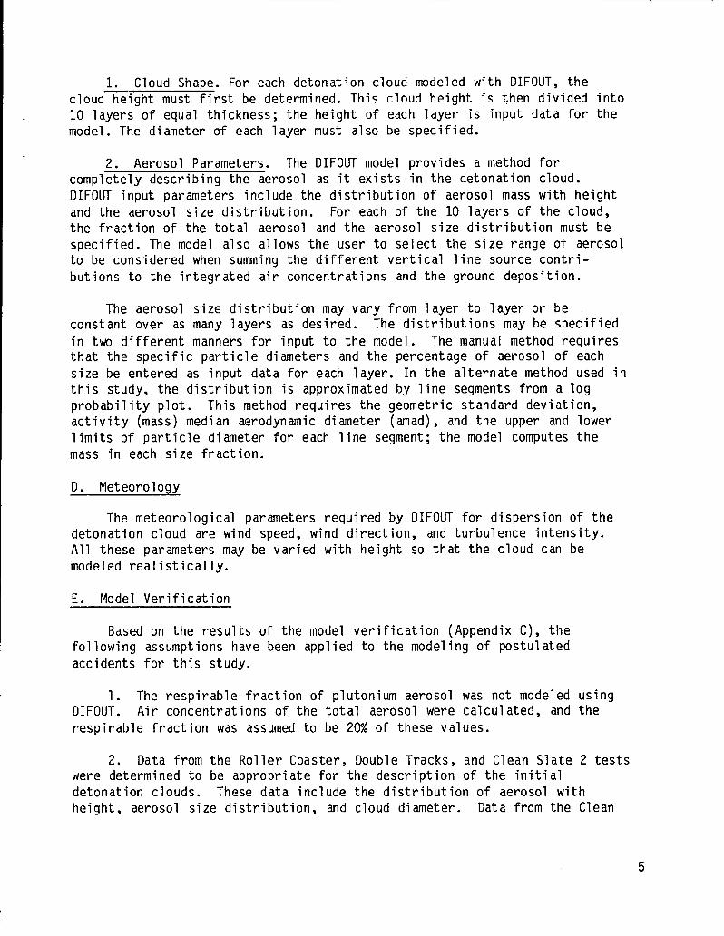
TOTAL .55 1.56 5.98 1.31 0.00 9.50
BURLINGTON 1967-1971
STABILITY D
WINO SPEED, KNOTS
TOTALDIR o-3 4-6 7-1o 11-16 17-22 22+
.45
.36
.47
.34
.62
.42
.50
.36
.92
.55
.35
.32
.34
.49
.36
.28
1.67.76.98
1.071.571.721.431.233.681.561.01
.761.011.401.51
.92
2.16.64.51.47.73.84.78.86
4.332.041.35
.691.162.482.931.77
.40
.05
.02
.03
.02
.08
.08
. OB
.43
.36
.25
.14
.40
.711.02
.50
.02
.01
.01
.010.00
.010.000.00
.02
.04
.03
.01
.08
.1212
:07
.55
4.771.862.05i.953.003.112.852.599.494.593.02i.973.055.275.983.59
NNNE
NEENE
EESE
SESSE
.07
.05
.07
.04
.06
.05
.06
.05s
Ssw12
:04.04.04.06.07.04.04
SwWsw
wWNW
NWNNW
4.57 59.13TOTAL .90 7.12 22.26 23.73
49

DIR
NNNE
NEENE
EESE
SESSE
sSsw
SwWsw
wWNW
NWNNW
TOTAL
o-3
.2913
:24.15.28.28.22.24.59.27.17.16.28.38.36.22
4.25
BURLINGTON 1967-1971
STA81LITV E
WINO SPEED, KNOTS
4-6 7-1o 11-16
.8835
:66.47.82.92.84.86
2.02.86.60.63.98.93
1.25.85
.83
.20
.19
.19
.36
.43
.28
.271.88
.98
.48
.37
.50
.97
.88
.46
0.000.000.000.000.000.000.000.000.000.000.000.000.000.000.000.00
13.93 9.26 0.00
17-22
0.000.000.000.000.000.000.000.000.000.000.000.000’.000.000.000.00
0.00
22+
0.000.000.000.000.000.000.000.000.000.000.000.000.000.000.000.00
0.00
TOTAL
2.00.68
1.09.81
1.461.631.341.374.502.111.251.161.762.272.501.53
27.44
50

HANFORO 1973-1975
STABILITY B
WIND SPEED, KNOTS
22+ TOTALo-3 4-6 7-1o 11-16 17-22
0.000.000.000.000.000.000.000.00O.GCI
.0217
:08.01.11.21.01
2.142.541.76
.94
.911.101.13
.62
.651.152.142.491.222.624.462.23
NNNE
NEENE
EESE
SE
.55
.79
.74
.33
.28
.44
.39
.17
.20
.15
.15
.2118
:15.30.39
1.161.12
.78
.53
.54
.60
.66
.34
.35
.50
.52
.48
.43
.651.251.33
.34
.4618
:08.09.06.08.08.08.27.50.76.30.75
1.33.42
.06
.16
.060.000.000.000.00
.03
.0215
:48.67.25.64.80.07
.03
.010.000.000.000.000.000.000.00
.06
.3229
:05.32.57.01
SSEs
SswSw
Wsww
WNWNW
NNW
.61 28.10TOTAL 5.42 lfl.24 5.78 3.39 1.66
HANFORD 1973-1975
STABILITY D
WINO SPEEO. KNOTS
DIR
N~E
E~~E
ESESE
SSEs
SswSw
Wsww
WNWNW
NNW
TOTAL
o-3 4-6 7-1o 11-16 17-22 22+ TOTAL
.54
.55
.54
.41
.42
.36
.48
.27
.25
.20
.27
.24
.25
.33
.41
.50
.39
.28
.21
:;:.34.28
17:20.21.25.30.45.81.96.63
.14
.16
.05
.03
.04
.08
.1011
:09.27.32.53.65
1.231.02
.32
.06
.04
.05
.010.00
.01
.01
.04
.08
.30
.60
.52
.381.33
.01
.01
.020.000.000.000.000.00
-05.17.35
17:05.62.65.02
0.000.000.000.000.000.000.000.00
.01
.1113
:06.01.08
0:::
1.141.04
.87
.61
.66
.79
.87
.59
.681.261.921.821.794.404.011.56
.86
.09
6.02 5.84 5.14 4.38 2.12 .51 24.01
51

HANFORD
STABILI”
WINO SPEED
1973-1975
Y MS
KNOTS
4-6 7-1o 11-16 17-22 22+ TOTALOIR o-3
1.28.65.58.55.62.91
i.651.541.571.622.824.745.998.886.632.06
.11
.07
.02
.03
.06
.11
.21
.39
.25
.28
.621.742.484.062.50
.46
.01
.Oi
.010.000.000.00
.03
.04
.11
.17
.43
.65
.341.42
.93
.04
.010.00
.020.000.000.00
.01
.03
.04
.1119
:09.02.25.14
0.00
0.000.000.000.000.000.000.00
.010.00
.06
.09
.020.00
.020.000.00
NNNE
NE
.79
.33
.27
.32
.30
.36
.72
.45
.54
.44
.59
.54
.67
.68
.77
.63
.36
.24
.26
.20
.26
.44
.68
.62
.63
.56
.901.702.482.452.29
.93
ENEE
ESESE
SSEs
SswSw
Wsww
WNWNW
NNW
13.39 4.f9 .91 .20 42.09TOTAL 8.40 15.00
HANFORD 1973-1975
STABILITY VS
WIND SPEED, KNOTS
OIR
N&w
ENE
E~E
s::s
SswSw
Wsw
WriwNW
NNW
TOTAL
o-3 4-6 7-10 11-16 17-22 22+ TOTAL
.08
.07
.05
.06
.06-07.11.07
11:08.08.07
:E.14.10
.04
.04
.03
.01
.02
.0214
:15.10.17.18.26.47.44.39.15
0.000.000.000.000.00
0.000.000.000.00
::ER0.000.000.000.000.00
.010.00
.010.000.00
0.000.000.000.000.000.000.000.000.000.000.000.00
::E0.000.00
0.000.000.000.000.000.000.000.000.000.000.000.000.000.000.000.00
12:11.08-07.08
0.00.02
.09
.27.03.01.02-05.39.21.78.43.01
.25
.22
.27
.31
.73
.781.32
.96
.26
4.34 2.61 1.95 .02 0.00 0.00 5.92
52

I
APPENDIX C
DIFOUT MODEL VERIFICATION STUDY
I. INTRODUCTION
DIFOUT (Luna 1969) was designed to simulate the dispersion of a cloud of
particulate material, as opposed to other dispersion models that treat alldispersed material as gas. The accidental releases postulated here dealstrictly with a particle cloud in which fission products are negligible.Since many particles produced in the accident would be quite large (up to1000 urn),they wuld fall out near the source. For example a 500-~m particle
thrown 300 m into the air would reach the ground in only 150 s. If a 5 m/swind were blowing at the time, the particle vmuld be carried only 750 mdownwind from its starting point. Since weapons operations (excludingtransportation) are conducted at locations well inside the site fence, thisparticle would fall onsite. The ultimate use of this analysis isinvestigation of offsite consequences of airborne plutonium inhaled by thepopulation or plutonium deposited on soil and buildings; therefore, it isimportant to use a realistic model that accounts for both fallout of largerparticles and dispersion of particles small enough to be inhaled.
Usefulness of the DIFOUT model depended on its ability to predictairborne concentrations and disposition with reasonable accuracy over thedesired range. The best way to verify its ability to calculate these valueswas to prepare input from experimental data obtained in the four ProjectRoller Coaster tests and compare the calculated results with the experimentalresults. The success or shortcomings detected in these comparisons alloweddetermination of applicability of the model to each postulated accident (thatis, virtually unrestricted release versus partial restriction by earthbunkering).
II. ROLLER COASTER SUMMARY
The Roller Coaster test series was conducted over the period May 15 toJune 9, 1963 (Shreve 1965) . Table C-I summarizes the major features of thesetests. The four tests were entitled Double Tracks, Clean Slate 1, CleanSlate 2, and Clean Slate 3. Double Tracks and Clean Slate 1 were unbunkeredtests performed on open pads. Although there was some uptake of soil withthese tests, fallout was not enhanced to the extent observed in the bunkeredtests, Clean Slate 2 and 3. Each test was conducted to simulate a storage ortransport detonation accident. One plutonium-containing device was includedin each array to permit radiometric tracing of the dispersed material. Whenmore than one device was used, the additional assemblies were identical inconfiguration and HE amounts but with the plutonium replaced with depleted
53

Test
Double Tracks
Clean Slate 1
Clean Slate 2
Clean Slate 3
TABLE C-I
SUMMARY OF ROLLER COASTER TEST FEATURES
Approximate High
P1acement
8-ft by 8-ft
steel plate
20-ft by 20-ft
concrete pad
Storage bunker
2-ft roof
Storage bunker
Cloud Explosive
Height (m) Amount (lb)
220 118
710 1062
440 2242
520 2242
Mean Wind
Speed (m/s)
8
7
4
2.58-ft roof
uranium. Therefore, clouds produced were of representative height without
spreading unnecessary quantities of plutonium. It should be noted, however,that the activity-height distribution may be significantly affected by theuse of one plutonium-bearing device in a multidevice array.
The early morning (predawn) hours were selected to yield morepredictable wind direction, air turbulence, and wind speed. Downwindinstrument arrays, including air samplers supported by a balloon curtain,obtained airborne particle concentrations in terms of time-integrated dosage(vg-s/m3). Dosages in this form allow calculation of plutonium mass taken inby a person or animal breathing at a specific rate.
The Roller Coaster tests were reasonably well instrumented to provide(1) the meteorological conditions existing at the time of the test, (2) theaerosol concentrations at points of interest downrange, (3) the depositedactivity at points of interest downrange, (4) the particle size distributionof the aerosol at various heights, and (5) the cloud shape and activitydistribution in the cloud. This supporting information, input into theDIFOUT model, allowed calculation of time-inteclrated aerosol concentration(or airborne-dosage indownwind. Cases whereresults and calculatedinput for the accidentDIFOUT was available.
Pg-s/m3) and deposition (ug/m2) at desired distancesagreement was best between experimental (measured)results provided a basis for choosing appropriatecase calculations. No other source of verification of
54

Applicabi’experimenter’smeteorological
ity of Roller Coaster input data was enhanced by thechoice of early morning to perform the tests at a time whenconditions would be neutral or stable (D, E, or F stability
class by Pasquill category) (Slade 1968). These same stability categorieswere chosen as representative of the median and unfavorable dispersionconditions under which all of the accident cases were analyzed.
The most noteworthy findings of the Roller Coaster tests were thefollowing.
(1) Increasing the amount of HE reduces the radiological hazards byincreasing the cloud height.
(2) Plutonium particle size distribution indicated that the respirablefraction (fraction of total aerosol mass associated with particles less than10-um Dae) was approximately 0.20 for plutonium.
(3) The activity median aerodynamic diameter of the respirable fractionappeared to be approximately 5 um. Geometric standard deviation wasapproximately 2.5.
(4) Most of the plutonium mass in the weapon-1 ike assembly wasaerosolized.
(5) Soil overburden provided both a cloud height suppression andscavenging of plutonium particles, causing particles to deposit nearer to thedetonation site than for the unbunkered shots. Overburden 2 ft thick wasalmost as effective as overburden 8 ft thick, partially because a m~”orportion of the material vented through the door.
III. UNBUNKERED DETONATIONS
The unbunkered shots from Roller Coaster (Double Tracks and Clean Slate1) offered experimental data for use in verification of the DIFOUT model asapplied to postulated accidents in unbunkered locations. The cloud heightscovered the range of interest (220 m for Double Tracks and 710 m for CleanSlate 1). Although the actual plutonium amounts involved in the tests remainclassified, normalized airborne and deposited plutonium dosages have beenpresented as dosage per kilogram dispersed under measured conditions. Fromthese normalized dosages, scaling to higher plutonium amounts in thepostulated accident cases can be done with reasonable accuracy if (1) theDIFOUT model can be shown to approximate the Roller Coaster experimentalresults and (2) the dispersion conditions of the accident cases are closeenough to the Roller Coaster conditions to be considered applicable. Theanalyses described briefly in the next two sections were performed to
55

determine whether the DIFOUT model using either Double Tracks or Clean Slatedispersion conditions would adequately describe dispersion and deposition forthe postulated accidents occurring in unbunkered locations.
A. Double Tracks
In this analysis and in Clean Slate 1 and 2 analyses, the cloud wasdivided into 10 horizontal layers of equal thickness. Each layer wasassigned an activity concentration fraction, diameter, particle sizedistribution, and meteorological parameters, all obtained from Roller Coasterdata.
1. Cloud Description. The Double Tracks test produced a cloud 220 mhigh, the lowest of the Roller Coaster series. The general outline of thecloud after growth from thermal buoyancy had ceased is shown in Fig. C-1(Beasley 1965). This outline derived from photographic reproductionpermitted scaling of the cloud diameters with height (see Table V for clouddiameters).
2. Meteorological Conditions. The meteorological conditions existingduring the test were summarized completely in a classified report (Stewart1969) and partially in an unclassified report (Church 1969). The parametersof interest were wind speed, wind direction, vertical turbulence intensity,and horizontal turbulence intensity at several elevations up to ultimate
250-~
500 -~
~ 200 - 400 -
%k~ 15(3 . 300
:
Gz 100 200 -n30d 50 - 100-
\\I Io
0 50 100 150 200 250
HORIZONTAL DIMENSION(METERS)
Fig. C-1. Outline of debris cloud (Double Tracks at 105 s afterdetonation; Clean Slate 2, 120 s).
56

TABLE C-II
DOUBLE TRACKS METEOROLOGICAL PARAMETERS
Wind Wind Vertical HorizontalDirection Speed Turbulence Turbulence
Height (m) (degrees E of N) (m/s) Intensity Intensity
2 350 5.2 0.038 0.07920 370 5.6 0.038 0.07950 350 6.4 0.038 0.079
100 345 7.0 0.038 0.079200 340 7.8 0.038 0.079
cloud height and measured near enough to the cloud path to be representative.Table C-II lists the meteorological parameters used in modeling IMubleTracks. Horizontal and vertical turbulence intensities are measures of thecrosswind and vertical fluctuations of the wind, respectively.
3. Activity Fraction with Height. Relatively minor amounts ofplutonium were detected in the bottom two or three layers of the cloud, thatis, in the stem up to 0.2 to 0.3 of the cloud height. Figure C-2 showscumulative fractions of total plutonium activity versus fraction of cloud
height from the Double Tracks test. This relationship is considered
applicable to low-to-intermediate cloud heights (say 150 to 450 m) from
unbunkered locations. The actual activity fractions used in the DoubleTracks analysis are listed in Table VII in the body of this report.
4. Aerosol Size Distribution. Size distributions of plutonium-bearingparticles produced in Roller Coaster tests were treated in detail in anunclassified report (Friend 1965); variability in air sampler data wastreated in greater detail by Luna (1971).
The particle size distribution in a newly formed cloud is subject tochange with time as (1) larger particles settle out and (2) agglomerationdepletes the cloud of smaller particles. With the passage of time, a morephysically stable aerosol forms as most of the large particles have settledout and dispersion of the cloud has reduced particle concentration to thepoint where agglomeration becomeswere made after that time interva’stabilized cloud. These wuld beoffsite but would not necessarilynear the detonation site. The Ro’
negligible. If aerosol size measurementsthey would be representative of the
~f interest in determining airborne dosagesprovide representative deposition amountsler Coaster particle size measurements were
57

O ~’-i------”~I I I [ I I I Io 0.1 0.2 0.3 0.4 0.5 0.6 0.?’ 0.8 0.9 1
FRACTION OF CLOUD HEIGHT
Fig. C-2. Distribution of plutonium with height for Double Tracks andClean Slate 2 tests.
made at 750 m and beyond, which provided the desired information for bothoffsite airborne dosage and offsite deposition calculations.
Active particles in each cloud were composed of plutonium alone orplutonium attached to inert particles. The Roller Coaster data were based onaerosols collected inertially, analyzed radiometrically for activity (mass)of plutonium, and reported in terms of activity associated with particles ofaerodynamically equivalent diameter. Although particles behaving aero-dynamically alike might not contain like amounts of plutonium, the particlesize distribution can be described most usefully in terms of an activity
(plutonium activity) aerodynamic equivalent diameter (Dae). The inertialtechniques for determining Dae were appropriate, without need to knowmicroscopic diameters, shapes, or actual densities of particles. The sizecharacteristics of a log normally distributed aerosol of mixed particles canthen be described in terms of the activity median aerodynamic diameter (amad)and geometric standard deviation (ug). As noted in the ICRP Task Group onLung Dynamics report , regional deposition in the lungs is relativelyinsensitive to changes in Ug, making it unnecessary to include u in the
9model (ICRP 1966).
58

I03 I1 I 1 I i 1 I I I i I 1 i I I 1 I i I
L
N
102 .
Io’ -
/
1=
o .1 J().01 0.1 0.5 2 10 30 50 70 90 98 99.8 99.99
PERCENT OF AEROSOL MASS IN PARTICLESSMALLER THAN THE STATED DIAMETER
Fig. C-3. Aerosol size distribution for Roller Coaster experiments (Luna1971) .
Curves expressing the distribution of mass associated with particleswith diameters ranging from 0.1 to 1000 w are shown in Fig. C-3. None of
the size distributions in the Roller Coaster series were log normallydistributed; that is, the natural logarithms of particle diameters were notnormally distributed. However, each size distribution, when plotted on a logprobability scale as used in Fig. C-3, could be approximated by severalstraight line segments, each covering an interval of particle size. The
DIFOUT model could accommodate a composite distribution expressed in thismanner. The particle size characteristics of these composite distributions(taken from more detailed curves than Fig. C-3) were as follows.
59

[Althoughbe an art
Range (un)amad (pm)
‘9 From To
9000 90 0.1 4.038 3.8 4.0 6048 1.8 60 1000
the 9000-Mn activity median aerodynamic diameter (amad) appears toficial value, it is the median extrapolated at a 50% probabil ity by
the line segment best fitting the distribution between 0.1 and 4.0 um.]These characteristics were used as input to verify the DIFOUT model. Asnoted earlier, these composite distributions represent the continuum ofparticle sizes from o.1- to 1000-pm Dae. The model used this particlesize range to calculate the total airborne dosage, the respirable airbornedosage, and the deposited dosage.
A complete input file for each of the Roller Coaster tests is providedin Appendix C, DIFOUT Input Files.
5. Selection of Median Respirable Diameter. For the purpose ofselecting an amad as input to the ICRP Task Group lung model (ICRP 1966), theRoller Coaster particle size distribution data were reviewed for consistencyof the respirable fraction. The referenced Roller Coaster reports stated 19to 26% of the total aerosol mass was under 10-um Dae; therefore, 19 to26% was respirable by nose breathing. Because 20% has been commonly statedas the respirable fraction, 20% was used throughout this analysis. To con-struct an assumed log normal distribution of the under 10-um Da parti-
cles, percentage values by mass corresponding to several sizes f2, 5, and 8Pm) were normalized as though they were percentages of the mass of the under10-wn distribution. From these data, the characteristics of the log normaldistribution under 10 urnwere derived. The amad of this distribution wasapproximately 5 um. Although 5 wn is the probable diameter of interest, ityields a comparatively low pulmonary deposition by the ICRP lung model calcu-lation. Although submicron particles yield highest pulmonary deposition, itwas considered overly conservative to choose a submicron particle size.Consequently, an intermediate size of 2 m was selected upon which to baseorgan dose calculations. Friend (1965) indicated diminishing particle size(Fig. C-4) with distance. At 5 km, a distance very likely to be offsite, theamad was projected to be approximately 2 um. Particle size information toallow projection of amad beyond 5 km was not available. Some furtherreduction in crnad(and possibly in,respirable fraction) at greater distancescould be expected as the last of the larger particles fall out of the cloud.However, deposition data presented later show over 90% of ground depositionwill have occurred by the time the cloud moved 5 km.
60

U
d
8-
7-
6-
5-
4-
3-
2-
1-
0 I I I 11 2 3 4 5
DISTANCE (kilometers)
Fig. C-4. Variation of median particle diameter with distance (Friend 1965).
Derivations of organ dose factors applied to the integratedconcentrations obtained from DIFOUT are described by Elder (1982B).
6. Calculated Versus Measured Dosages. Peak dosages of total aerosoland respirable aerosol from Double Tracks calculated by DIFOUT model areshown as functions of distance in Fig. C-5.
Agreement between the calculated and measured amounts of total aerosolwas reasonably good. The dosage was underestimated no more than a factor of2 (this under 1000 m); beyond 2000 m the dosage was overestimated by no morethan a factor of 2.
Calculated values of peak respirable dosage were gross underestimates ofthe measured dosage out to 7000 to 8000 m. At 1000 m the difference was afactor of 10 to 20. This underestimation of respirable dosage made therespirable calculation of dubious value.
Deposited dosages, shown in Fig. C-6, were in reasonable agreement overthe range of interest. The dip in measured dosage from 400 to 2000 m was not
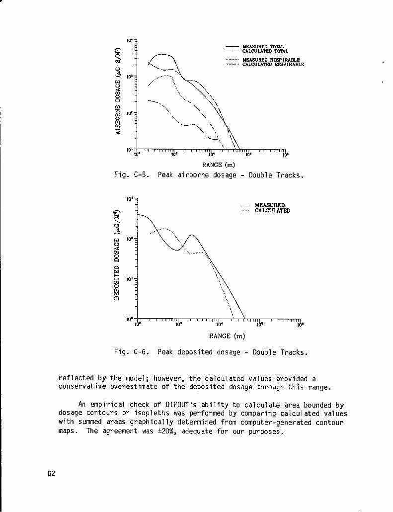
reflected byconservative
—— MEASURED TQTALCALCULATEDTOTAL
---------MEASURED RESPIRABLE—- CALCULATEDRSPIRABLE
10”3
g
&I
\ —.~ *@
.----------...w ...C!J ,..””
...s ..,.8 ...
2 ~~.3m \E2 ‘—’\’’’’’’’’’”..
10’ I II1111111 T1IIiIll 1 tI11111 1 1 1 Ill-q
ld Iv1
lot lh~ ld
RANGE (m)
Fig. C-5. Peak airborne dosage - Double Tracks.
ElC!J
il
— MEASURED----- CALCULATED
I&=
101=
$.,10’J 1 t 1 1 1 1111 I 1 I 1 1 1111 1 1 I 1 1
NY1111 1 1
10=1 111111
10* lo~ 1(Y
RANGE (m)
Fig. C-6. Peak deposited dosage - Double Tracks.
the model; however, the calculated values provided aoverestimate of the deposited dosage through this range.
An empirical check of DIFOUT’S ability to calculate area bounded bydosage contours or isopleths was performed by comparing calculated valueswith summed areas graphically determined from computer-generated contourmaps. The agreement was *20%, adequate for our purposes.
62

Id
~-
,!
— MEASURED-I RABLE
‘“’”n
‘— CALCULATEDRESPIRABLE
: ---------MEASUREDTOTALAEROSOLMY i ‘L —. CALCULATEDlWTALAERC50L
~
cdCJ
$0c1
wzlxomlx
Fig. C-7. Peak airborne dosage - Clean S’ate 1.
B. Clean Slate 1
Clean Slate 1, another unbunkered test, also offered-the opportunity forinput to the postulated accident cases, particularly where high clouds (moreHE) were postulated. However, as shown in Fig. C-7, major disagreementexists between the measured and calculated values of total aerosol andrespirable aerosol, particularly within 4000 m of the detonation site.Beyond 4000 m, the model overestimates total aerosol by a factor of 10. Theoverestimation of total aerosol by the model may not be caused by the modelat all; rather, overestimation may be caused by a lower than expected aerosolconcentration resulting from the Roller Coaster test arrangement. It issuspected thatdevices causedhigh elevationplutonium withaccidents.
ringing the only plutonium-containing test device with otherthe plutonium in the Clean Slate 1 cloud to be lifted to ain the center of the cloud. Therefore, the distribution ofheight probably would not be representative of the postulated
The respirable aerosol curve was in reasonable agreement over the shortrange where the measured and calculated values overlapped and both showed adip at 4000 to 6000 m. However, the model indicated a respirable aerosolpeak 60 000 to 80 000 m away which, if real, was missed by the downwindsampler array.
Figure C-8 shows that deposition is calculated in reasonable agreementwith measured values 1000 m and beyond. Inside 1000 m, the dosage is grosslyunderestimated.
63

—MEASURED DEPOSITION----CALCULATED DEPOSITION
Id
101=
Id 1 1 1 111111 1 1 1 111111 1 I 1 111111 1 1 1 IllTq
NY Id lot 106 IdRANGE (m)
C-8. Peak deposited dosage - Clean Slate 1.
In general, the Clean Slate 1 test results were not consistent with themodel, discouraging any use of these measured conditions as input to themodel for accident analysis. Consequently, the meteorological data,particle size characteristics, and clouds are not described in detail here.However, a complete input file for each of the DIFOUT runs is provided inAppendix C, DIFOUT Input Files.
Iv. BUNKERED DETONATIONS
The bunkered shots of Roller Coaster (Clean Slate 2 and 3) offeredexperimental data for use in verification of the DIFOUT model as applied topostulated accidents in bunkered locations. The only major differencebetween these two tests was the thickness of the overburden (2 ft for CleanSlate 2; 8 ft for Clean Slate 3). Since the results were similar for thesetests, only Clean Slate 2 will be covered in detail in this Appendix. Theadditional overburden apparently had little effect.
Clean Slate 2
Cloud Description. The cloudgeneral outline of the cloud afterdiffers from Double Tracks only instem and larger top.
height of Clean Slate 2 was 440 m. Thebuoyant growth had ceased (Fig. C-1)that Clean Slate 2 has a better defined
Meteorological Conditions. Table C-III lists the meteorologicalconditions used in modeling Clean Slate 2 (Church 1969).
64

I
TABLE C-III
CLEAN SLATE 2 METEOROLOGICAL PARAMETERS
Height (m)
22550
125175225275325375425
WindDirection
(degrees E of N)
360325325325290300300300340340
WindSpeed .(ills)
2.13.03.24.27.25.03.02.01.52.0
VerticalTurbulenceIntensity
0.0780.0780.0360.0360.0360.0360.0360.0360.0360.036
“HorizontalTurbulenceIntensity
0.0700.0700.0180.0180.0180.0180.0180.0180.0180.018
Activity Fraction with Height. Figure C-2 shows the relationshipbetween cumulative plutonium activity and fractional cloud height for CleanSlate 2. Somewhat higher activity amounts were measured in the lower layersof the Clean Slate 2.~loud thanwould be expected where more sothe plutonium particles. Actua”analysis are listed in Table VI
Aerosol Size Distribution.distribution was similar to tha
were measured in the Double Tracks cloud, as1 particles were present to aid in scavengingactivity fractions used in the Clean Slate 2
in the body of this report.
Analysis of Clean Slate 2 aerosol sizedescribed earlier for Double Tracks, except
the particle size information (unclassified) was found in classified reportAWRE T6/69 (Stewart 1969). Overall size distribution was shown earlier inFig. C-3. The distribution was approximated by two line segments asfollows.
Range (urn)amad (urn)
‘9From To
.—
39 7.8 0.1 4241 2.3 42 1000
A complete input file for the Clean Slate 2 test is provided in AppendixC, DIFOUT Input Files.
65

+
3EASURED TOTAL AEROX)L‘---_CALCULATEO TOTAL AEROSOL
lo.~KY lo~ 10+ KY KP
RANGE (m)
Fig. C-9. Peak airborne dosage - Clean S1ate 2.
Calculated Versus Measured Dosages. Peak dosages of total aerosol fromthe Clean S1ate 2 test data are shown as functions of distance in Fig. C-9.Agreement was not exceptionally good. However, beyond 600 m the model eitherpredicted closely or overestimated the measured value. Beyond 4000 m, thedosage was consistently overestimated by a factor of 10. This discrepancymay have been caused by better scavenging processes than a simple sedimenta-tion and turbulent dispersion depletion model would predict.
Peak deposition is shown as a function of distance in Fig. C-10. Themodel underestimated peak deposition over the entire range but only by afactor of 1.5 to 2.5 beyond 1500 m, the shortest distance to the siteboundary for any of the accident cases. Therefore, for offsite dosagecalculations, the model is considered to adequately estimate deposition.
v. SUMMARY AND CONCLUSIONS
Airborne and deposited plutonium dosages expected from the RollerCoaster test series of 1963 were calculated using the DIFOUT dispersionmodel. Meteorological parameters, cloud descriptions, and particle sizecharacteristics from this series of four plutonium dispersion tests were usedto model the tests as carefully as possible. The calculated values of totalairborne dosage and deposition dosage adequately approximated or conserva-tively overestimated the measured values. Poor agreement between measuredand calculated respirable airborne dosage suggests that an alternative methodbe used to estimate respirable airborne dosage, that is, the total airbornedosage multiplied by a respirable fraction of 20%.
66

nGI*zon.Mcl
—MEASURED DEPOSITION----CALCULATED DEPOS1TION
Id=
......
............
Id= ....
101 1 1 I11111[ I 1 TII111 I 1 11111111(Y Id :.4 MY
RANGE (m)
Fig. C-10. Peak deposition - Clean Slate 2.
The verification process indicated that parameters and conditionssimilar to those from the Double Tracks test performed in an unbunkeredlocation would be suitable for estimating dosages from accidents inunbunkered assembly/disassembly areas. Parameters from the Clean Slate 2test performed in an earth-covered bunker would be suitable for DIFOUTestimation of dosages from the accidents in earth-bunkered locations.
REFERENCES
Beasley 1965: R. R. Beasley, “Operation Roller Coaster: Technical Photo-graphy,” Department of Defense report POR-2519 (August 1965).
Church 1969: H. W. Church, “Cloud Rise from High Explosives Detonations,”Sandia Laboratories report SC-RR-68-903 (May 1969) .
Elder 19828: J. C. Elder, R. H. Olsher, and J. M. Graf, “SupplementaryDocumentation for an Environmental Impact Statement Regarding thePantex Plant: Radiological Consequences of Immediate Inhalation ofPlutonium Dispersed by Postulated Accidents,” Los Alamos NationalLaboratory report LA-9445 -PNTX-F (1982).
Friend 1965: J. P. Friend and l).M. C. Thomas, ’’The Determination of theParticle Size Distribution of the Particulate Material CollectedDuring the Double Tracks and Clean Slate 1 Events of Operation RollerCoaster,” Atomic Weapons Research Establishment (UK) report AWRE O-20/65 (February 1965) .
67

ICRP 1966: International Commission on Radiological Protection, Task Groupon Lung Dynamics, P. E. Morrow, Chairman, “Deposition and RetentionModels for Internal Dosimetry of the Human Respiratory Tract,” HealthPhys. 12, 173-207 (1966).—
Luna 1969: R. E. Luna and H. W. Church, “DIFOUT: A Model for Computationof Aerosol Transport and Diffusion in the Atmosphere,” SandiaLaboratories report SC-RR-68-555 (January 1969).
Luna 1971: R. E. Luna, H. W. Church, and J. D. Shreve, “Variability of AirSampler Data,” Atmos. Environ., Vol. 5, 579-597 (1971).
Shreve 1965: J. l).Shreve, Jr., “Operation Roller Coaster: ScientificDirector’s Summary Report,” Department of Defense report DASA-1644(June 1965) .
Slade 1968: D. H. Slade, “Meteorology and Atomic Energy,” US Atomic EnergyCommission report TID-24190 (July 1968).
Stewart 1969: K. Stewart, “Roller Coaster Summary Report,” Atomic WeaponsResearch Establishment (UK) report, AWRE T6/69, Secret Restricted Data(1969).
68

DIFOUT INPUT FILES
69

3 VERIFICATION PROBLEM FUR OIFOUT6.25E+2
2.1
0.1-?5.121.
78..01.14
2
5:2350..079.079.038
3200.
64000.91
lE-64:OE-660.E-6
51O.E-6
53.OE+O
5I.OE+l
51.OE+O
1.70E+;10
2.OE+I1.
9110.
200.91.67..01.09
520.5.6
370..038.079.038
50$80000.
310
4.OE-660.E-6
400.E-63
1OOO.E-6
1.OE+l
3.OE+I
1.OE+l5.OE-I2.0E+4
1.0E+9MICROGRAMS2!6.
25.216.
71.1
.0651
50.6.4
350.
. (379
.038
1000.
19.OE-338.E-648.E-6
1OOO.E-6
3.OE+l
1 .0E+2
1.0E+21
50.
115.
.085
100..7.0
345.
.079
.038
2000.
1 .0E+069.OE+l3.8E+01.8E+0
1.0E+2
3.0E+2
1.0E+31
USING OT OATA
75.
128.
.12
200.7.8
340.
.(379
.038
4000.
444
3.0E+2
1.0E+3
1.0E+4
100. 125. 150.
91. 34. 71.
.14 .17 .17
8000. 16000. 32000.

2.1
0.600.155.i41.
.0018.153
22.
600.
;:;55.
325..14.14
.061.25
.0443
1000.100ooo.
9
1. E-O;200. E-6
92
.05 E-621 O. E-6
9
.OIE-0~80. E-06
9
.07E-0~
3 VERIFICATION PROBLEM FOR OIFOUT USING CSI OATA6.25E+2 2.OE+l t.oE+9MIcRoGRAMs
1.11
7%:154.
26..0027
.04510
25.700.
2.87.0
350.325.
.25.061.061.044.044
to2000.
120000.21
120.E-65
1O.E-65
1.OE-15
1.OE-1
1.45E+;10
200.E-6f500.E-6
2
2t0.E-i600.E-6
23
80.E-61OOO.E-6
210
120.E-61OOO.E-6
600.E-:
3.OE-1
1.0E405.OE-12.0E+4
710.
30.710.250.
.00:51.
50.
5.2
395.
.061
.044
4000.
t2.E-t
350.E-6
24.8E-2
210.E-6
34000.E-6
180.E-6
438.E-675.E-6
1 .OE+O
1.OE+l1
100.
340.
.029
too.
5.5
325.
.061
.044
8000.
1. OE +0638.E+O1 .4E+0
1 .0E+648.E+o3.5E+0
1 .C)E+640.E+o2.2E+0
1.0E+65.4E+02.lE+O
3.OE+O
1.0E+21
200.
252.
.102
200.
7.2
325.
.061
.044
16000.
1500.
300.
300.
.153
300.
8.0
325.
.061
.044
32000.
44
44
44
44
1.OE+l
1.0E+3
145.
400.
289.
. t94
400.
8.2
325.
.061
.044
64000.
500.
291.
.216
500.
7.0
325.
.061
.044
80000.

1 4 VERIFICATION PROBLEM FOR OIFOUT USING CS1 DATA6.25E+2
2.1
0.480.155.141.
.0018. 153
2
62:1.27.055.
325..14. i4
.061.25
.0443
100.64000.
91
1.E-07200.E-6
92
.05E-621O.E-6
9
.OIE-0~80. E-06
94
.07E-06120.E-6
5-1000.E-6
51.OE-2
31 .45E+2
fo
2.OE+l1.
1::556.154.
. o%.045
$0
7%:
H350.325.
.25.061.061.044.044
10500.
80000.2f
200.E-61500.E-6
2
21O.E-;600.E-6
23
80.E-61OOO.E-6
210
120.E-61000..E-6
1
1.OE-1
2.0E+4
1.0E+9MICROGRAMS560.
30.560.250.
.00:s1.
50.
5.2
315.
.061
.044
1000.
12.E-1
350. E -6
24.8E-2
21O.E-6
34000.E-6
180.E-6
438.E-675.E-6
1.OE+O1
100.
340.
.029
100.
5.5
325.
.061
.044
2000.
1. OE+0638.E+O1. 4E+0
1.0E+648.E+o3.5E+0
1 .0E+640.E+O2.2E+0
1 .0E+65.4E+02.lE+O
1.OE+l1
176.
252.
.102
252.
300.
. 153
200.
7.2
325.
300.
8.0
325.
.061
.044
.061
.044
4000.
44
44
44
44
t.0E+2
328.
289.
.194
400.
8.2
325.
.061
.044
~6000.
404.
291.
.2f6
500.
7.0
325.
.061
.044
32000.
72

4 VERIFICATION PROBLEM FOR OIFOUT USING CS2 DATA0.70E+2
f.1
0.343.155.189.
.01
.122
37; :2.11.5
360.340..078.078.036
.07.018
3
64% :91
lE-64i.E-6
5600.E-6
51.OE-3
51 .OE+o
11 .50E+2
10
2.OE+l1.11
to.391.162.122.
.01
.0410
25.425.
3.02.0
325.340.
.07.078.036
.07.018
10
60% :2
1042.E-6
KK)O.E-62
-1000.E-6
1.OE-2
1.OE+l5.OE-12.0E+4
1.0E+9MICROGRAMS440.
30.440.135.
1..06
1.
50.
3.2
325.
.036
.018
1000.
139.E-64~.E-6
1.OE-1
1 .0E+21
100.
68.
.11
125.
4.2
325.
.036
.018
2000.
1. 0E+067.8E+02.3E+0
1 .OE+o
1.0E+31
149.
61.
. 12
175.
7.2
290.
.036
.018
4000.
44
1.OE+l
1.0E+4
198.
81.
.15
225.
5.0
300.
.036
.018
8000.
8
247.
209.
.18
275.
3.0
300.
.036
.018
16000.
295.
250.
.19
325.
2.0
300.
.036
.018
32000.
73

?4T2sPW Range Prim Coda
Pdmad in the United Stma of A- ,,
Awiltbk from
Nadmml Tachmcsl !nfornmtkn SaIW&
US Dapsnment of Commerce
S285 Pon Royd Road
S@@Jd. VA 2’2161
NTIS
price code
00102s AO1
026030 A03
05 I 07s AM
076.100 ,405
101.12s A06
[:6.1S0 A07
1s1.17s
176.200
20112s116-2S0231273276.100
A06
AW
A 10
.411
A12
A13
Pa8e Range
301.125326.1:0351.3753?64CQ401.4254:6.4s0
NTIS
P!iae coda
NTIS
PsSa Ran-e Ptica Co&
A14
A 1S
A16
All
A18
A19
4s147s A20476.S00 A21
Soi 52s A22S26-SS0 A235s1.s75 A24
S76+.00 A25
601 up” AW
“Contact NTIS for ● price quote.

. ..”.. ..’