gyrocenter gauge kinetic theory and algorithm for … gauge kinetic theory and algorithm for...
TRANSCRIPT
Gyrocenter Gauge Kinetic Theory and Algorithm for Radio-Frequency Waves in Plasmas
Hong QinPrinceton Plasma Physics Laboratory, Princeton University
Numerical Flow Models for Controlled Fusion
16-20 April, 2007Porquerolles, France
http://www.pppl.gov/~hongqin/Gyrokinetics.php
2
Acknowledgement
Thank Prof. Ronald C. Davidson and Dr. Janardhan Manickam for their continuous support.
Thank Drs. John Cary, Peter J. Catto, Bruce I. Cohen, Ronald Cohen, Gregory W. Hammet, Nathaniel J. Fisch, Roman A. Kolesnikov, William M. Nevins, W. Wei-li Lee, Cynthia K. Phillips, David N. Smithe, Edward A. Startsev, William M. Tang, and Ernest J. Valeo for fruitful discussions.
US DOE contract AC02-76CH03073.
3
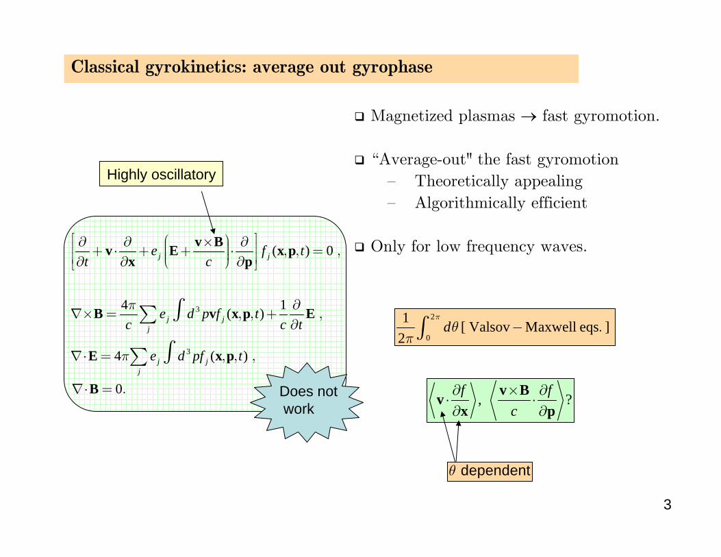
Classical gyrokinetics: average out gyrophase
Magnetized plasmas → fast gyromotion.
“Average-out" the fast gyromotion– Theoretically appealing– Algorithmically efficient
Only for low frequency waves.
2
0
1 [ Valsov Maxwell eqs ]2
dπ
θπ
− .∫
, ?f fc
v Bvx p
∂ × ∂⋅ ⋅∂ ∂
Highly oscillatory
dependentθ
Does notwork
3
3
( ) 0
4 1( )
4 ( )
0
π
π
⎡ ⎤⎛ ⎞∂ ∂ × ∂⎟⎜⎢ ⎥+ ⋅ + + ⋅ , , = ,⎟⎜ ⎟⎜⎢ ⎥⎝ ⎠∂ ∂ ∂⎣ ⎦
∂∇× = , , + ,
∂
∇⋅ = , , ,
∇⋅ = .
∫∑
∫∑
j j
j jj
j jj
e f tt c
e d p f tc c t
e d pf t
v Bv E x px p
B v x p E
E x p
B
4
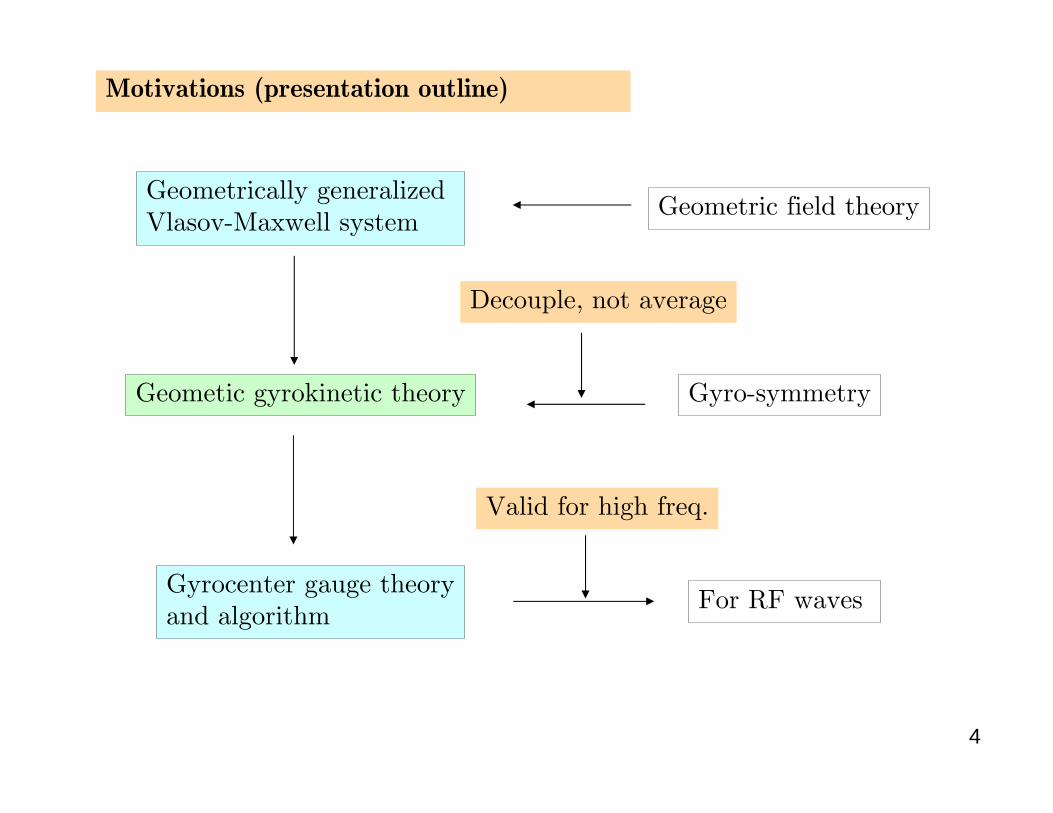
Motivations (presentation outline)
Geometrically generalized Vlasov-Maxwell system
Geometic gyrokinetic theory
Gyrocenter gauge theoryand algorithm
Geometric field theory
Gyro-symmetry
For RF waves
Decouple, not average
Valid for high freq.
5
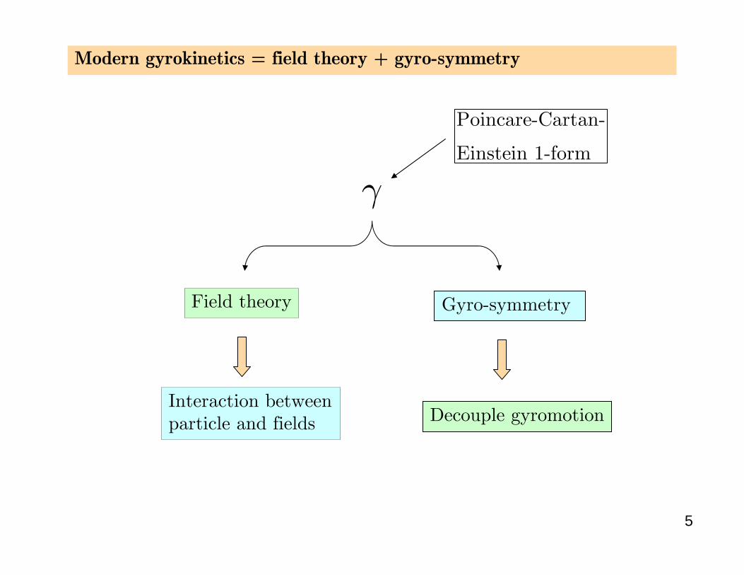
Modern gyrokinetics = field theory + gyro-symmetry
Gyro-symmetry
Decouple gyromotion
Field theory
Interaction between particle and fields
γ
Poincare-Cartan-
Einstein 1-form
6
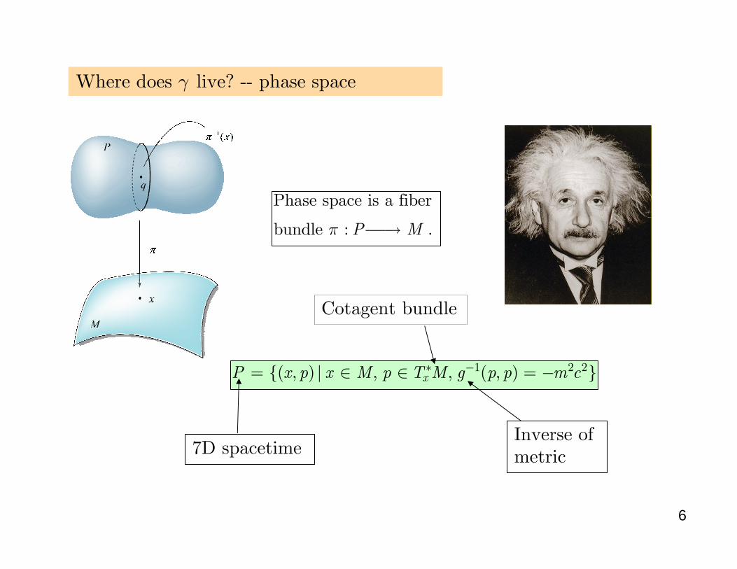
1 2 2( ) ( ) xP x p x M p T M g p p m c∗ −= , | ∈ , ∈ , , = −
7D spacetimeInverse of metric
Phase space is a fiber
bundle P Mπ : ⎯→ .
Cotagent bundle
Where does live? -- phase spaceγ
7
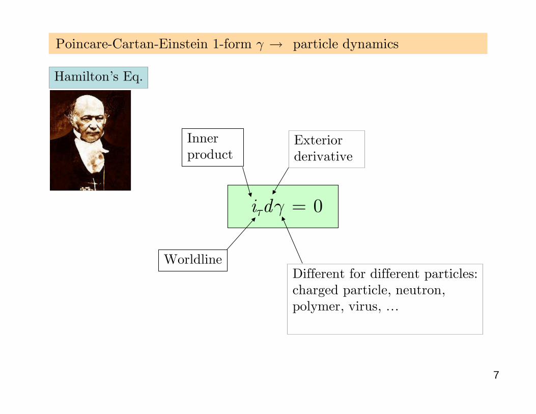
0i dτ γ =
Worldline
Inner product
Exterior derivative
Different for different particles:charged particle, neutron,polymer, virus, …
Poincare-Cartan-Einstein 1-form particle dynamicsγ →
Hamilton’s Eq.
8
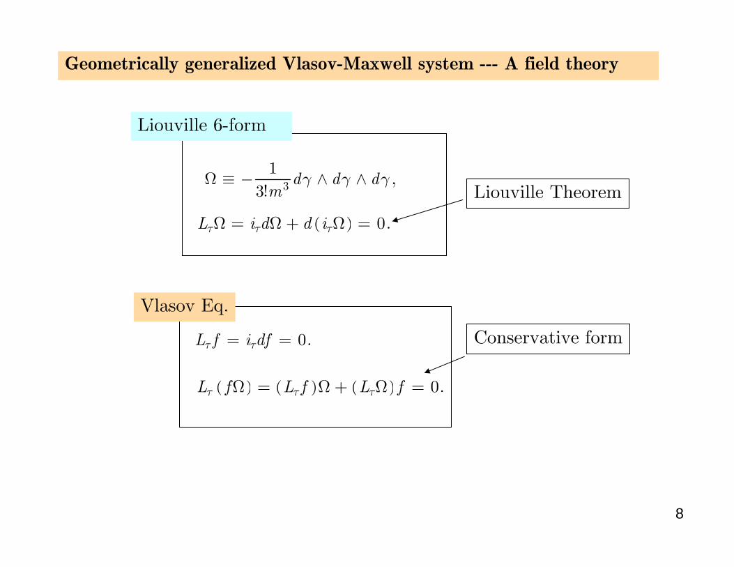
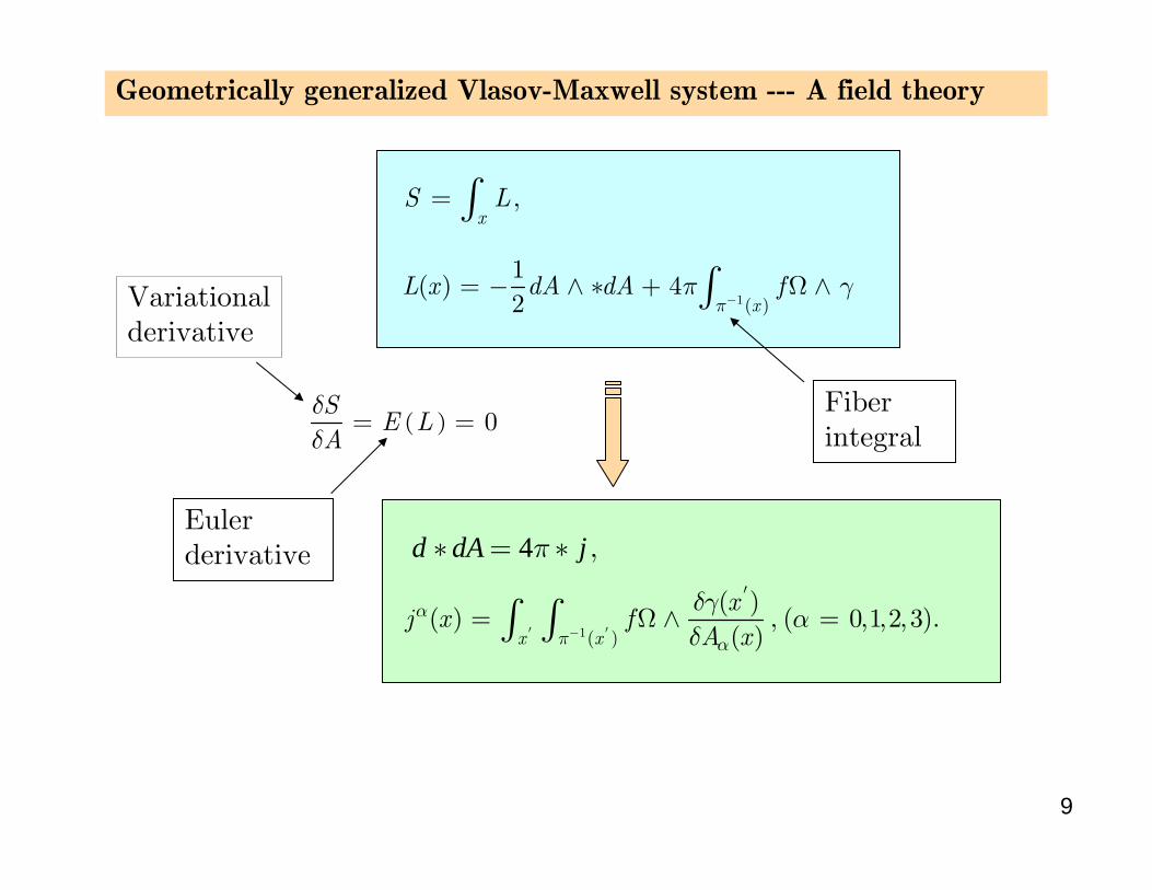
Geometrically generalized Vlasov-Maxwell system --- A field theory
31
,3
d d dm
γ γ γΩ ≡ − ∧ ∧!
0L f i dfτ τ= = .
( ) ( ) ( ) 0L f L f L fτ τ τΩ = Ω + Ω = .
( ) 0.L i d d iτ τ τΩ = Ω + Ω =
Liouville 6-form
Vlasov Eq.
Liouville Theorem
Conservative form
9
Geometrically generalized Vlasov-Maxwell system --- A field theory
4d dA jπ∗ = ∗ ,
xS L= ,∫
1( )
1( ) 4
2 xL x dA dA f
ππ γ
−= − ∧ ∗ + Ω ∧∫
1( )
( )( ) ( 0 1 2 3)
( )x x
xj x f
A xα
π α
δγα
δ′ − ′
′= Ω ∧ , = , , , .∫ ∫
( ) 0S
E LAδδ
= =
Variationalderivative
Fiber integral
Euler derivative
10
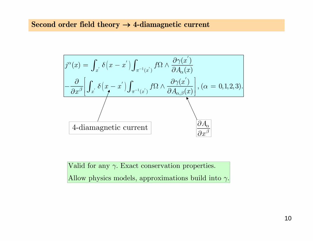
Second order field theory → 4-diamagnetic current
( )
( )
1
1
( )
( )
( )( )
( )
( )( 0 1 2 3)
( )
x x
x x
xj x x x f
A x
xx x f
A xx
απ α
β π α β
γδ
γδ α
′ − ′
′ − ′
′′
′′
,
∂= − Ω ∧
∂⎡ ⎤∂ ∂⎢ ⎥− − Ω ∧ , = , , , .⎢ ⎥∂∂ ⎣ ⎦
∫ ∫
∫ ∫
Axαβ
∂∂
4-diamagnetic current
Valid for any . Exact conservation properties.
Allow physics models, approximations build into .
γ
γ
11
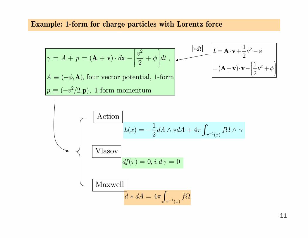
Example: 1-form for charge particles with Lorentz force
2
2
( )2
( ), four vector potential, 1-form
( 2 ), 1-form momentum
vA p d dt
A
p v
γ φ
φ
⎡ ⎤⎢ ⎥= + = + ⋅ − + ,⎢ ⎥⎣ ⎦
≡ − ,
≡ − / ,
A v x
A
p
( )
2
2
12
12
L v
v
φ
φ
= ⋅ + −
⎛ ⎞⎟⎜= + ⋅ − + ⎟⎜ ⎟⎜⎝ ⎠
A v
A v v
dt×
1( )
1( ) 4
2 xL x dA dA f
ππ γ
−= − ∧ ∗ + Ω ∧∫
1( )4
xd dA f
ππ
−∗ = Ω∫
( ) 0 0df i dττ γ= , =
Action
Vlasov
Maxwell
12
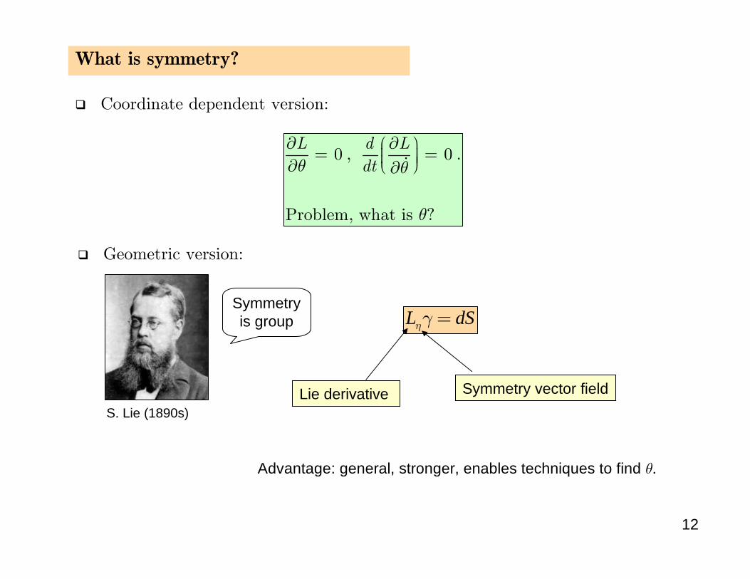
What is symmetry?
Coordinate dependent version:
Geometric version:
L dSηγ =
Lie derivative Symmetry vector field
0 0 .
Problem, what is ?
L d Ldtθ θ
θ
∂ ∂⎛ ⎞⎟⎜= , =⎟⎟⎜⎝ ⎠∂ ∂
S. Lie (1890s)
.Advantage: general, stronger, enables techniques to find θ
Symmetry is group
13
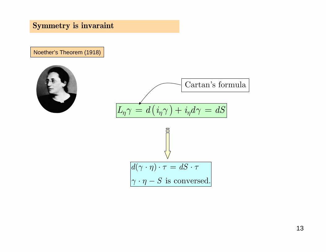
Symmetry is invaraint
( )L d i i d dSη η ηγ γ γ= + =
Noether’s Theorem (1918)
Cartan’s formula
( )
is conversed.
d dS
S
γ η τ τ
γ η
⋅ ⋅ = ⋅
⋅ −
14
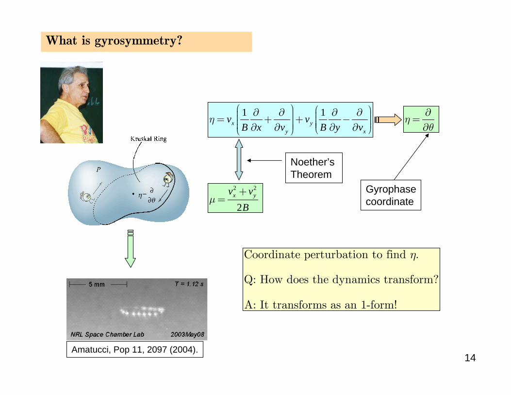
What is gyrosymmetry?
1 1x y
y x
v vB x v B y v
η⎛ ⎞ ⎛ ⎞∂ ∂ ∂ ∂⎟⎜ ⎟⎜⎟ ⎟⎜= + + −⎜⎟ ⎟⎜ ⎜⎟ ⎟⎜⎟∂ ∂ ∂ ∂⎜ ⎝ ⎠⎝ ⎠
Noether’sTheorem
Gyrophasecoordinate
Coordinate perturbation to find .
Q: How does the dynamics transform?
A: It transforms as an 1-form!
η
2 2
2x yv v
Bµ
+=
ηθ∂
=∂
Amatucci, Pop 11, 2097 (2004).
15
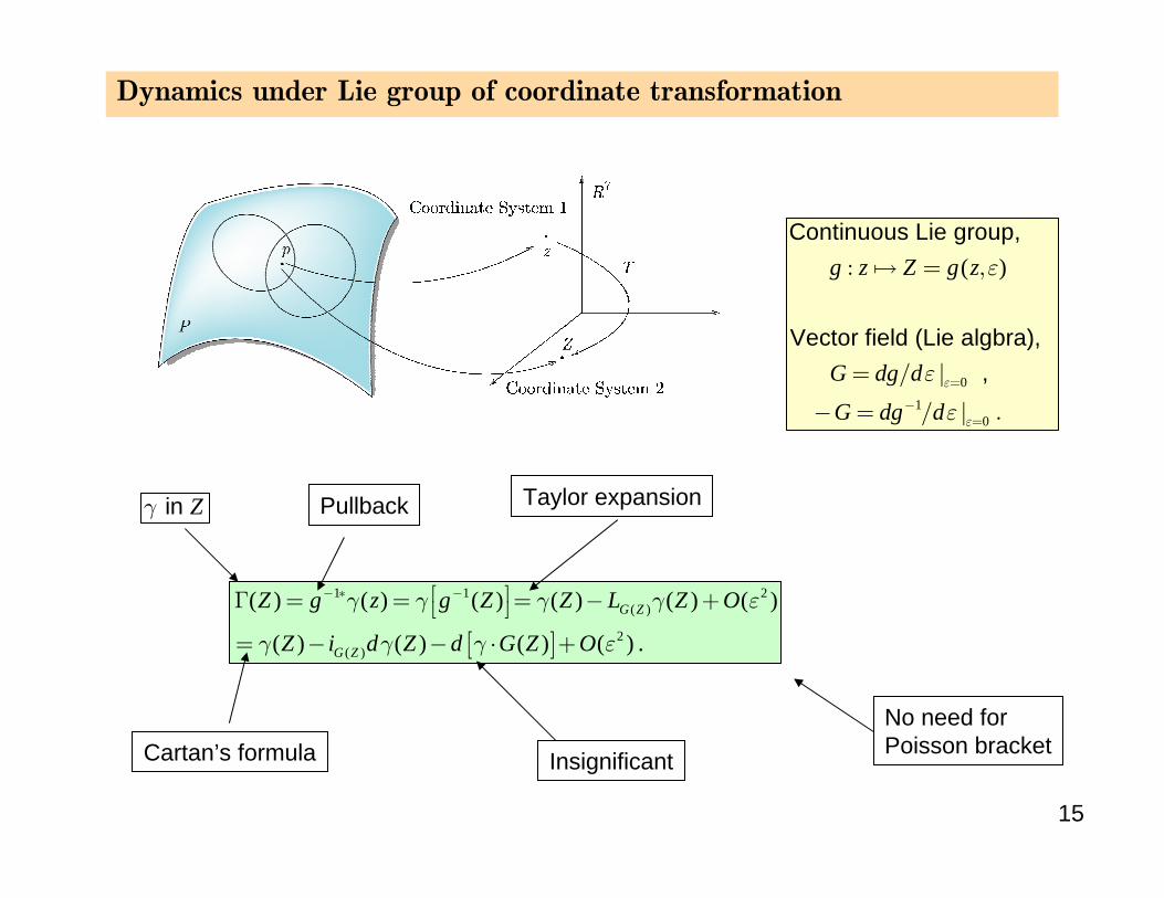
Dynamics under Lie group of coordinate transformation
[ ]
1 1 2( )
2( )
( ) ( ) ( ) ( ) ( ) ( )
( ) ( ) ( ) ( ) .G Z
G Z
Z g z g Z Z L Z O
Z i d Z d G Z O
γ γ γ γ ε
γ γ γ ε
− ∗ −⎡ ⎤Γ = = = − +⎣ ⎦= − − ⋅ +
0
10
( )Continuous Lie group,
Vector field (Lie algbra), ,
g z Z g z
G dg d
G dg dε
ε
ε
ε
ε=
−=
: = ,
= / |
− = / | .
Zγ in Pullback
Cartan’s formula Insignificant
No need for Poisson bracket
Taylor expansion
16
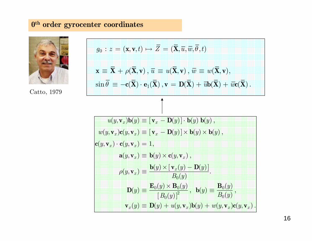
0th order gyrocenter coordinates
Catto, 1979
[ ]
[ ]
[ ]
[ ]
0
0 0 02
00
( ) ( ) ( ) ( ) ( )
( ) ( ) ( ) ( ) ( )
( ) ( ) 1
( ) ( ) ( )
( ) ( ) ( )( )
( )
( ) ( ) ( )( ) ( )
( )( )
( ) ( ) ( ) ( ) ( )
x x
x x x
x x
x x
xx
x x x
u y y y y y
w y y y y y
y y
y y y
y y yy
B y
y y yy y
B yB y
y y u y y w y
ρ
, ≡ − ⋅ ,
, , ≡ − × × ,
, ⋅ , = ,
, ≡ × , ,
× −, ≡ .
×≡ , ≡ ,
≡ + , + ,
v b v D b b
v c v v D b b
c v c v
a v b c v
b v Dv
E B BD b
v D v b v c( )xy, .v
0 ( ) ( )g z t Z u w tθ: = , , = , , , ,x v X
1
( ) ( ) ( ),
sin ( ) ( ) ( ) ( ) ( )
u u w w
u w
ρ
θ
≡ + , , ≡ , , ≡ ,
≡ − ⋅ , = + + .
x X X v X v X v
c X e X v D X b X c X
17
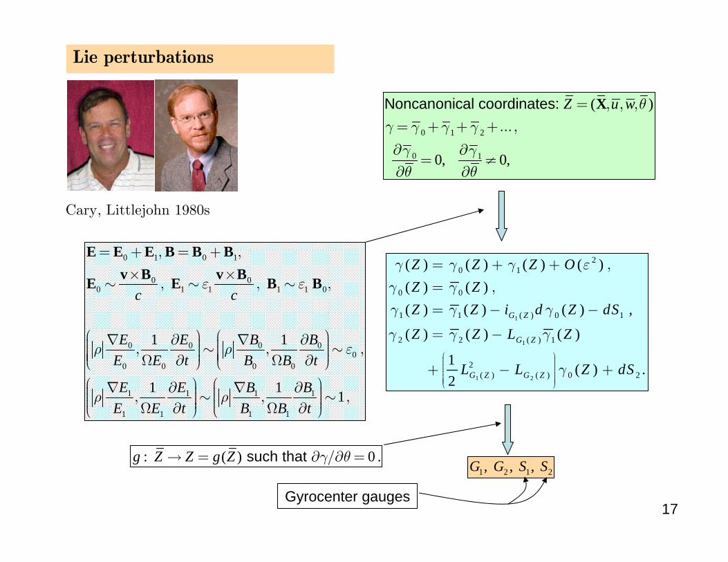
Lie perturbations
0 1 2
0 1
( )
0, 0,
Noncanonical coordinates:
Z u w θγ γ γ γ
γ γθ θ
= , , ,= + + +...,
∂ ∂= ≠
∂ ∂
X
: ( ) 0 .g Z Z g Z such that γ θ→ = ∂ /∂ =
1
1
1 2
20 1
0 0
1 1 ( ) 0 1
2 2 ( ) 1
2( ) ( ) 0 2
( ) ( ) ( ) ( )( ) ( )( ) ( ) ( ) ,
( ) ( ) ( )
1 ( ) .2
G Z
G Z
G Z G Z
Z Z Z OZ ZZ Z i d Z dS
Z Z L Z
L L Z dS
γ γ γ ε
γ γγ γ γ
γ γ γ
γ⎛ ⎞⎟⎜ ⎟⎜ ⎟⎜ ⎟⎜ ⎟⎜ ⎟⎜ ⎟⎟⎜ ⎟⎜⎝ ⎠
= + + ,
= ,
= − −
= −
+ − +
1 2 1 2, , , G G S S
Gyrocenter gauges
0 1 0 1
0 00 1 1 1 1 0
0 0 0 00
0 0 0 0
1 1 1 1
1 1 1 1
1 1
1 1 1
ε ε
ρ ρ ε
ρ ρ
= + , = + ,
× ×, , ,
⎛ ⎞ ⎛ ⎞∇ ∂ ∇ ∂⎟ ⎟⎜ ⎜⎟ ⎟, , ,⎜ ⎜⎟ ⎟⎜ ⎜⎟ ⎟⎜ ⎜Ω ∂ Ω ∂⎝ ⎠ ⎝ ⎠⎛ ⎞ ⎛ ⎞∇ ∂ ∇ ∂⎟ ⎟⎜ ⎜⎟ ⎟, , ,⎜ ⎜⎟ ⎟⎜ ⎜⎟ ⎟Ω ∂ Ω ∂⎝ ⎠ ⎝ ⎠
∼ ∼ ∼
∼ ∼
∼ ∼
c c
E E B BE E t B B t
E E B BE E t B B t
E E E B B Bv B v BE E B B
Cary, Littlejohn 1980s
18
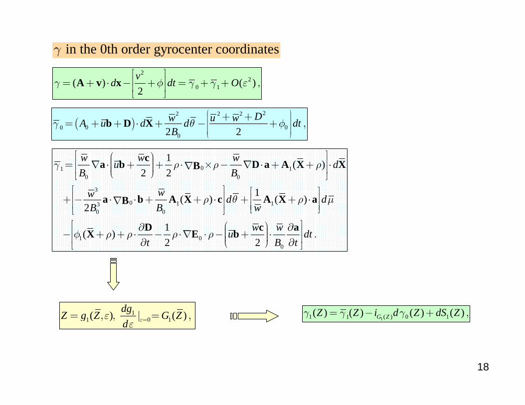
22
0 1( ) ( )2
γ φ εγ γ⎡ ⎤⎢ ⎥= + ⋅ − + = + + ,⎢ ⎥⎣ ⎦
vd dt OA v x
( )22 2 2
0 0002 2
Dw u wA u d d dtB
θ φγ⎛ ⎞⎟⎜ ⎟⎜ ⎟⎜ ⎟⎜ ⎟⎜ ⎟⎜ ⎟⎟⎜ ⎟⎜ ⎟⎜⎝ ⎠
+ += + + ⋅ + − + ,b D X
0 110 0
3
0 1 130 0
1 00
1 ( )2 2
1( ) ( )2
1( )2 2
ρ ρ ργ
ρ θ ρ µ
φ ρ ρ ρ ρ
⎡ ⎤⎛ ⎞⎟⎜⎢ ⎥= ∇ ⋅ + + ⋅ × − ∇ ⋅ + + ⋅∇⎟⎜ ⎟⎜⎢ ⎥⎝ ⎠⎣ ⎦⎡ ⎤ ⎡ ⎤⎢ ⎥ ⎢ ⎥+ − ⋅ ⋅ + + ⋅ + + ⋅∇⎢ ⎥ ⎢ ⎥⎣ ⎦⎣ ⎦⎡ ⎤⎛ ⎞∂ ∂⎟⎜⎢ ⎥− + + ⋅ − ⋅∇ ⋅ − + ⋅ .⎟⎜ ⎟⎜⎢ ⎥⎝ ⎠∂ ∂⎣ ⎦
w w wu dB B
ww d dB B w
w wu dtt B t
ca b D a A X XB
a b A X c A X aB
D c aX E b
11 0 1( ) ( )dgZ g Z G Z
d εεε == , , | = , 11 ( ) 0 11( ) ( ) ( ) ( )G ZZ Z i d Z dS Zγ γγ= − + ,
in the 0th order gyrocenter coordinatesγ
19
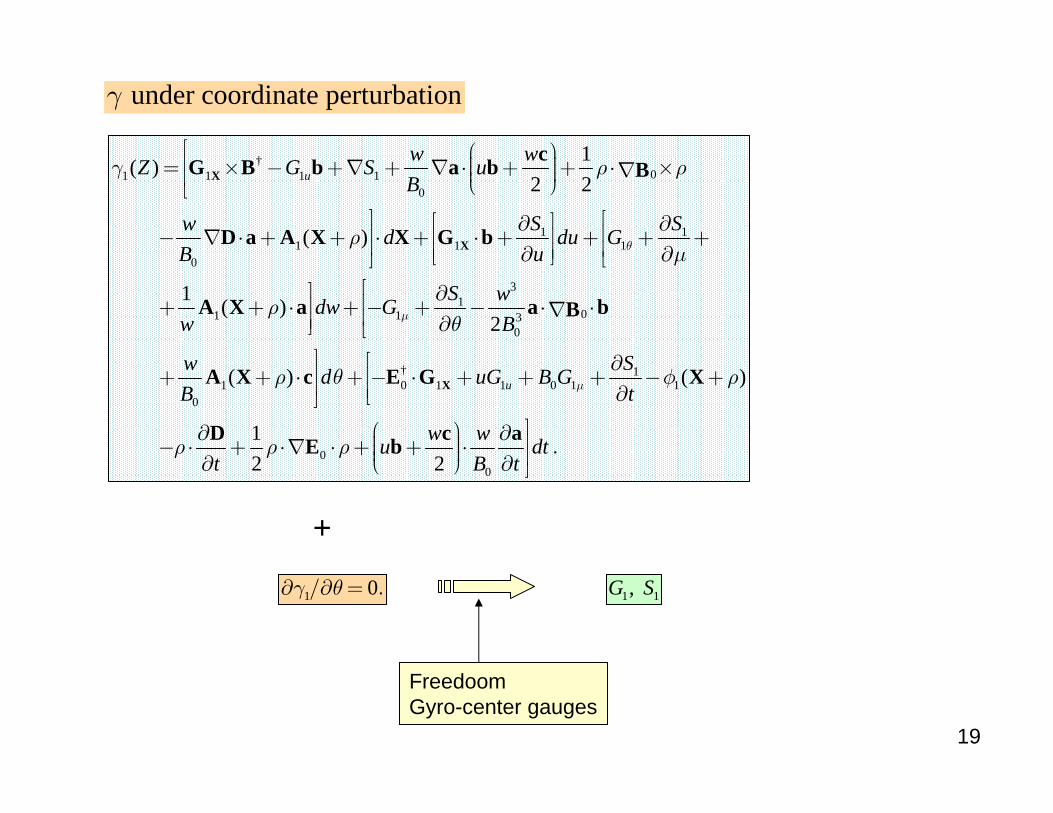
†01 1 1 1
0
1 11 1 1
0
31
01 1 30
†1 0 1 1
0
1( )2 2
( )
1 ( )2
( )
θ
µ
γ ρ ρ
ρµ
ρθ
ρ θ
⎡ ⎛ ⎞⎟⎜⎢= × − +∇ + ∇ ⋅ + + ⋅ ×∇⎟⎜ ⎟⎜⎢ ⎝ ⎠⎣⎤ ⎡⎡ ⎤∂ ∂⎥ ⎢⎢ ⎥− ∇ ⋅ + + ⋅ + ⋅ + + + +⎥ ⎢⎢ ⎥∂ ∂⎣ ⎦ ⎣⎦⎡⎤ ∂⎢⎥+ + ⋅ + − + − ⋅ ⋅∇⎢⎥ ∂⎦ ⎣
⎤⎥+ + ⋅ + − ⋅ + +⎥⎦
u
u
w wZ G S uB
S Sw d du GB u
S wdw Gw B
w d uG BB
X
X
X
cG B b a b B
D a A X X G b
A X a a bB
A X c E G 10 1 1
00
( )
12 2
µ φ ρ
ρ ρ ρ
⎡ ∂⎢ + − +⎢ ∂⎣
⎤⎛ ⎞∂ ∂⎟⎜ ⎥− ⋅ + ⋅∇ ⋅ + + ⋅ .⎟⎜ ⎟⎜ ⎥⎝ ⎠∂ ∂ ⎦
SGt
w wu dtt B t
X
D c aE b
1 0γ θ∂ /∂ = .
+
1 1, G S
FreedoomGyro-center gauges
under coordinate perturbationγ
20
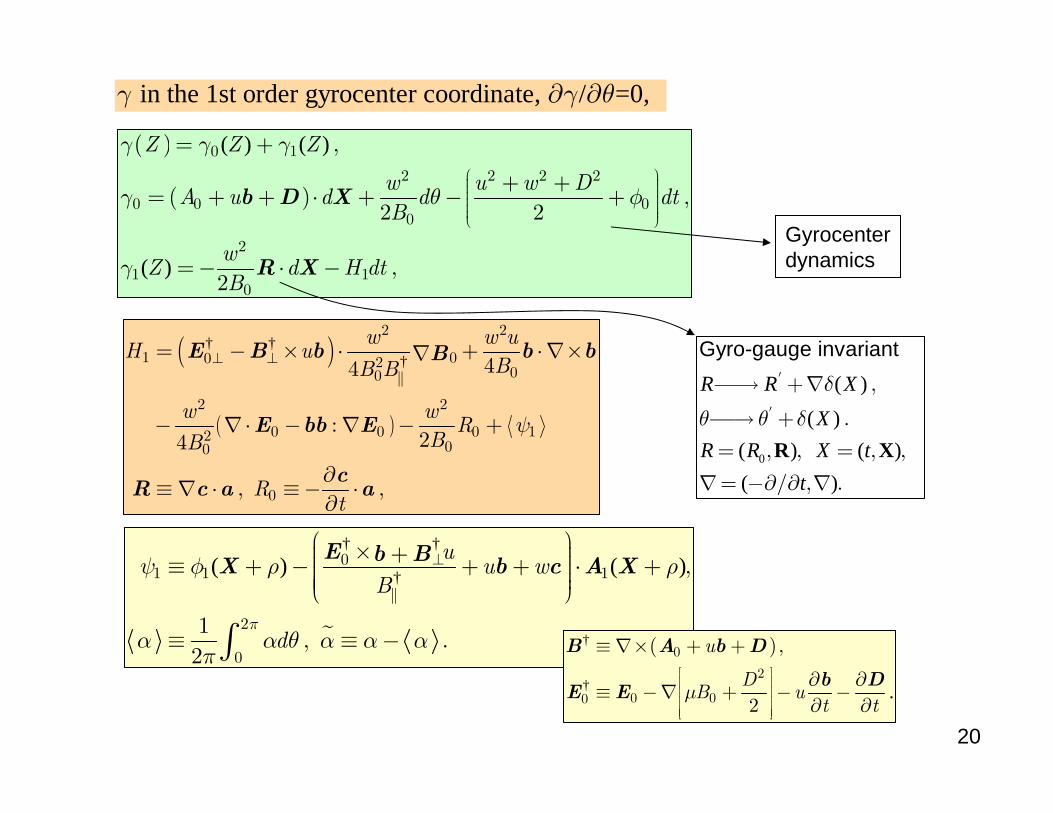
( )
( )
( ) ( )
( )
0 1
2 2 2 2
0 0 00
2
1 10
2 2
2
Z Z Z
w u w DA u d d dt
B
wZ d H dt
B
γ γ γ
γ θ φ
γ
⎛ ⎞⎟⎜ ⎟⎜ ⎟⎜ ⎟⎜ ⎟⎜ ⎟⎟⎜⎝ ⎠
= + ,
+ += + + ⋅ + − + ,
=− ⋅ − ,
b D X
R X
( )
( )
† ††
2 2
1 00 200
2 2
0 0 0 1200
0
44
24
w w uH u
BB B
w wR
BB
Rt
ψ
⊥ ⊥= − × ⋅ + ⋅∇×∇
− ∇⋅ − : ∇ − +
∂≡∇ ⋅ , ≡− ⋅ ,
∂
E B b b bB
E bb E
cR c a a
† †
†( ) ( )01 1 1
2
0
12
uu w
B
dπ
ψ φ ρ ρ
α α θ α α απ
⊥⎛ ⎞× ⎟+⎜ ⎟⎜≡ + − + + ⋅ + ,⎟⎜ ⎟⎜ ⎟⎜⎝ ⎠
≡ , ≡ − .∫
E b BX b c A X
Gyrocenterdynamics
in the 1st order gyrocenter coordinate, / =0, γ γ θ∂ ∂
0
( )( )
( ) ( )( )
Gyro-gauge invariant
R R XX
R R X tt
δ
θ θ δ
′
′
⎯→ +∇ ,
⎯→ + .= , , = , ,
∇= −∂/∂ ,∇ .
R X
( )†
† .
0
2
0 00 2
u
DB u
t tµ⎡ ⎤⎢ ⎥⎢ ⎥⎢ ⎥⎢ ⎥⎣ ⎦
≡ ∇× + + ,
∂ ∂≡ −∇ + − −
∂ ∂
B A b D
b DE E
21
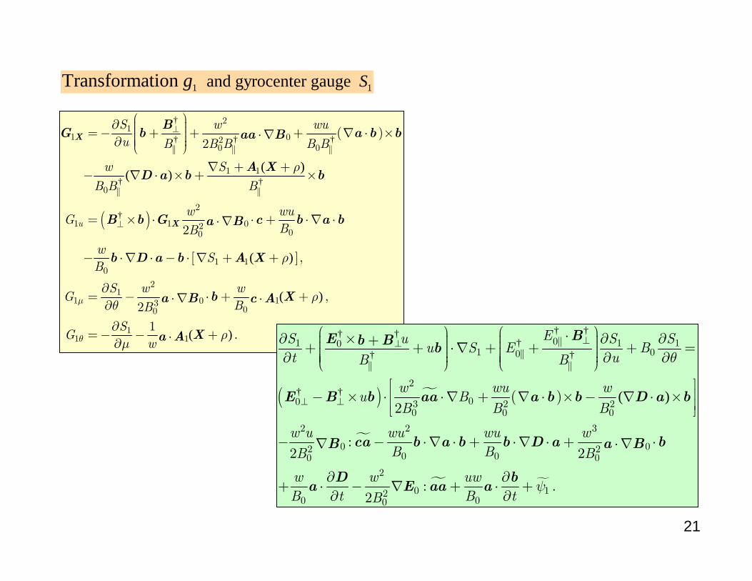
( )
( )
[ ]
†
† † †
† †
†
( )( )
( )
( )
21
1 020 0
1 1
0
2
1 1 0200
1 10
21
11 0300
1
2
2
2
u
S w wuu B B B B B
w S
B B B
w wuG
BB
wS
B
S w wG
BB
SG
µ
θ
ρ
ρ
ρθ
⊥
⊥
⎛ ⎞∂ ⎟⎜ ⎟⎜=− + + + ∇ ⋅ ×⋅∇⎟⎜ ⎟∂ ⎜ ⎟⎜⎝ ⎠
∇ + +− ∇ ⋅ × + ×
= × ⋅ ⋅ + ⋅∇ ⋅⋅∇
− ⋅∇ ⋅ − ⋅ ∇ + + ,
∂= − ⋅ + + ,⋅∇ ⋅∂
∂=−
X
X
BG b a b baa B
A XD a b b
B b G c b a ba B
b D a b A X
b Xa B c A
( )11
1w
ρµ
− + .⋅∂Xa A
( ) ( )
† †† ††
† †
† † ( )
01 1 101 00
2
00 3 2 20 0 0
2 2 3
0 02 20 00 0
0
2
2 2
ES u S Su S E B
t uB B
w wu wu B
B B B
w u wu wu wB BB B
wB
θ⊥⊥
⊥ ⊥
⎛ ⎞ ⎛ ⎞⋅∂ × ∂ ∂⎟ ⎟+⎜ ⎜⎟ ⎟⎜ ⎜+ + ⋅∇ + + + =⎟ ⎟⎜ ⎜⎟ ⎟∂ ∂ ∂⎜ ⎜⎟ ⎟⎜ ⎜⎝ ⎠ ⎝ ⎠⎡ ⎤⎢ ⎥− × ⋅ ⋅∇ + ∇ ⋅ × − ∇ ⋅ ×⎢ ⎥⎣ ⎦
− : − ⋅∇ ⋅ + ⋅∇ ⋅ + ⋅∇ ⋅∇
∂+ ⋅
BE b B b
E B b aa a b b D a b
ca b a b b D a bB a B
a2
0 12002
w uwt B tB
ψ∂
− ∇ : + ⋅ + .∂ ∂D b
E aa a
1 1 and gyrocenter gauge Transformation Sg
22
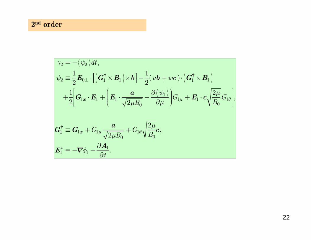
2nd order
( ) ( ) ( )† †
†
2 2
2 0 1 11 1
11 1 1 1 1 1
00
1 1 1100
11 1
1 12 2
1 22 2
22
dt
u w
G GBB
G GBB
t
µ θ
µ θ
γ ψ
ψ
ψ µµµ
µµ
φ
⊥
⎡ ⎤⎢ ⎥⎢ ⎥⎢ ⎥⎢ ⎥⎣ ⎦
∗
=− ,
⎡ ⎤≡ ⋅ × × − + ⋅ ×⎣ ⎦
⎛ ⎞∂ ⎟⎜+ ⋅ + ⋅ − + ⋅ ,⎟⎜ ⎟⎜ ∂⎝ ⎠
≡ + + ,
∂≡− − .
∂
x
x
E G B b b c G B
aG E E E c
aG G c
AE ∇
23
Perturbation techniques — quest of good coordinates
Peanuts by Charles Schulz. Reprint permitted by UFS, Inc.
24
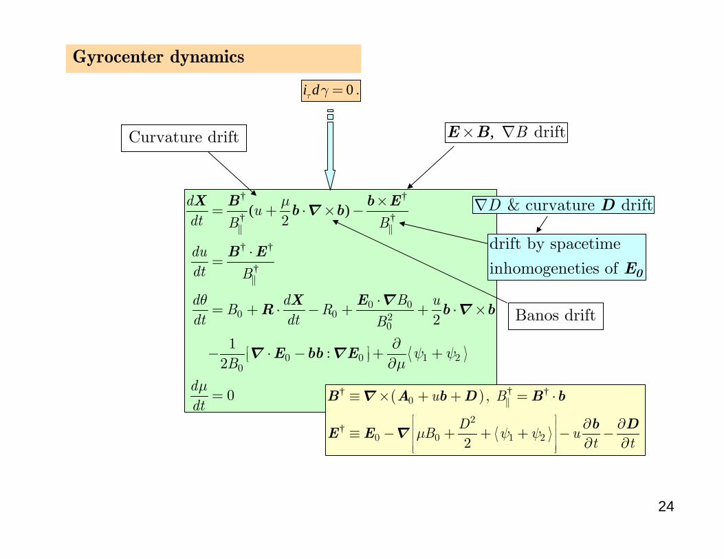
Gyrocenter dynamics
0i dτ γ = .
† †
† †
† †
†
( )
0 00 0 2
0
0 0 1 20
2
2
12
0
du
dt B B
dudt B
d d B uB R
dt dt B
B
ddt
µ
θ
ψ ψµ
µ
⎡ ⎤⎢ ⎥⎣ ⎦
×= + ⋅ × −
⋅=
⋅= + ⋅ − + + ⋅ ×
∂− ⋅ − : + +
∂
=
X B b Eb b
B E
X ER b b
E bb E
∇
∇∇
∇ ∇
( ) †† †
†
0
2
0 0 1 2
2
u B
DB u
t tµ ψ ψ⎡ ⎤⎢ ⎥⎢ ⎥⎢ ⎥⎢ ⎥⎣ ⎦
≡ × + + , = ⋅
∂ ∂≡ − + + + − −
∂ ∂
B A b D B b
b DE E
∇
∇
Banos drift
, driftB× ∇E B
drift by spacetime
inhomogeneties of 0E
Curvature drift
& curvature driftD∇ D
25
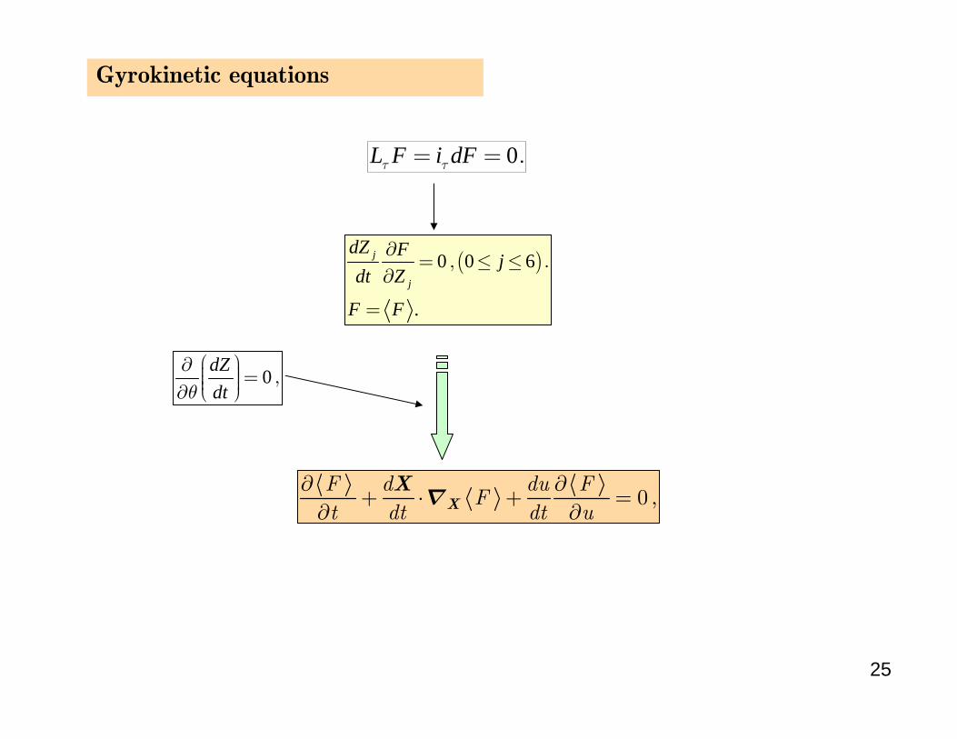
Gyrokinetic equations
( )0 0 6
.
∂= , ≤ ≤ .
∂
=
j
j
dZ F jdt Z
F F
0dZdtθ
⎛ ⎞∂ ⎟⎜ = ,⎟⎜ ⎟⎜⎝ ⎠∂
0F d du F
Ft dt dt u
∂ ∂+ ⋅ + = ,
∂ ∂XX
∇
0τ τ= = .L F i dF
26
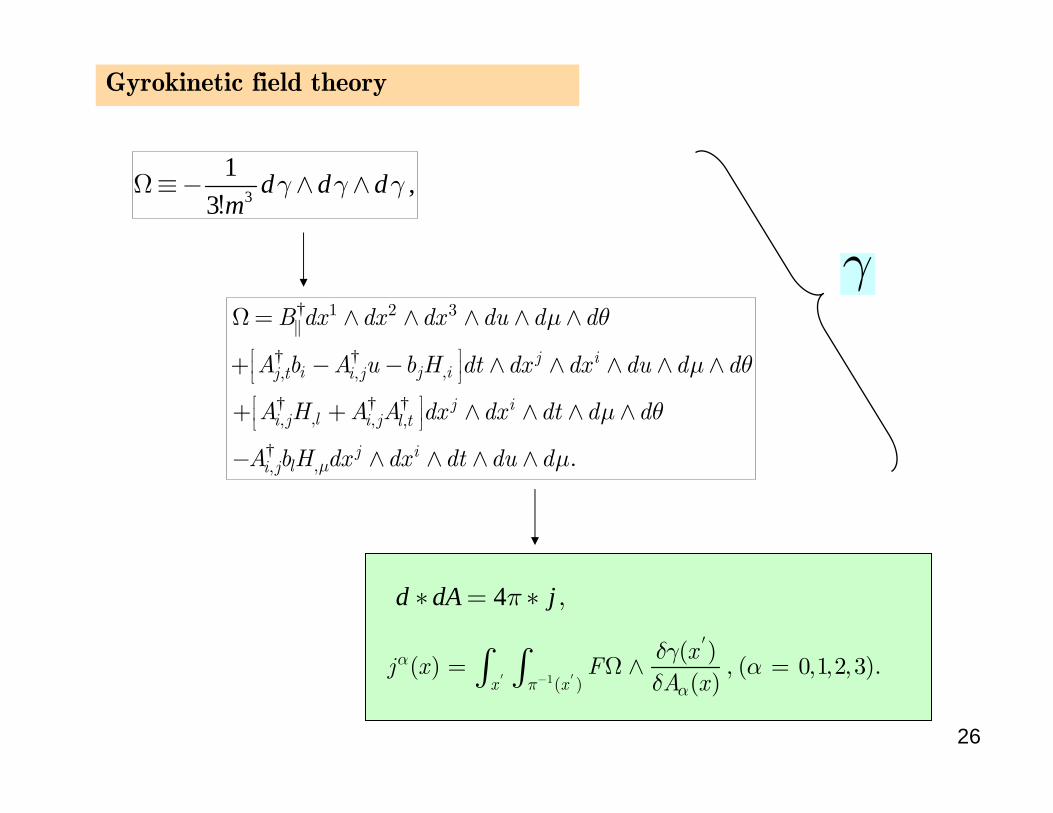
Gyrokinetic field theory
3
1 ,3
d d dm
γ γ γΩ≡− ∧ ∧!
†
† †
† † †
†
1 2 3
j ii j ij t i j
j ili j i j l t
j ili j
B dx dx dx du d d
A b A u b H dt dx dx du d d
A H A A dx dx dt d d
A bH dx dx dt du dµ
µ θ
µ θ
µ θ
µ
⎡ ⎤⎢ ⎥,, ,⎣ ⎦⎡ ⎤⎢ ⎥,, , ,⎣ ⎦
,,
Ω = ∧ ∧ ∧ ∧ ∧
+ − − ∧ ∧ ∧ ∧ ∧
+ + ∧ ∧ ∧ ∧
− ∧ ∧ ∧ ∧ .
4d dA jπ∗ = ∗ ,
1( )
( )( ) ( 0 1 2 3)
( )x x
xj x F
A xα
π α
δγα
δ′ − ′
′= Ω ∧ , = , , , .∫ ∫
γ
27
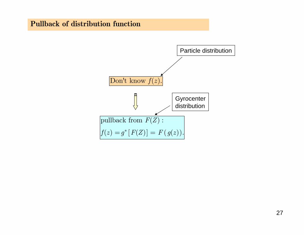
Pullback of distribution function
[ ] ( )
pullback from ( ) :
( ) ( ) ( )
F Z
f z g F Z F g z∗= = .
Particle distribution
Don't know ( ).f z
Gyrocenterdistribution
28
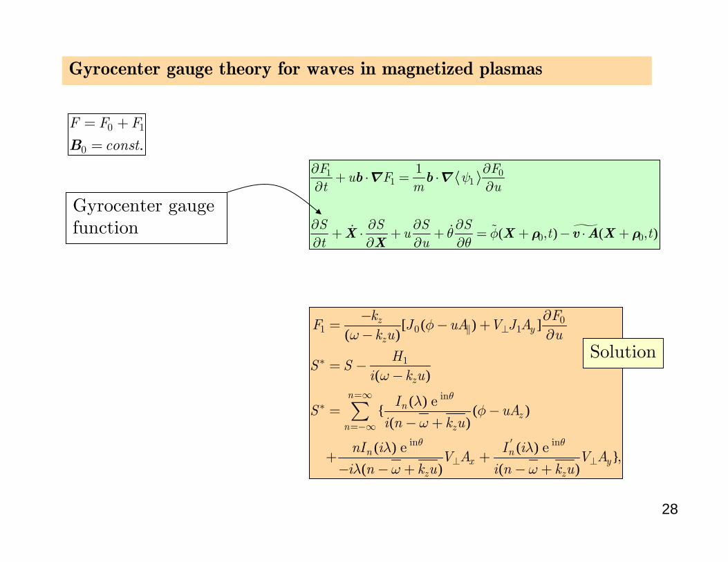
( ) ( )
1 01 1
0 0
1F Fu F
t m u
S S S Su t t
t u
ψ
θ φθ
∂ ∂+ ⋅ = ⋅
∂ ∂
∂ ∂ ∂ ∂+ ⋅ + + = + , − ⋅ + ,
∂ ∂ ∂ ∂
b b
X X v A XX
∇ ∇
ρ ρ
Gyrocenter gauge theory for waves in magnetized plasmas
.0 1
0
F F F
const
= +=B
Gyrocenter gauge function
[ ( ) ]( )
( )
( ) ( )( )
( ) ( ) ( ) ( )
01 0 1
1
in
in in
e
e e
zy
z
z
nn
zn z
n nx y
z z
k FF J uA V J A
k u u
HS S
i k u
IS uA
i n k u
nI i I iV A V A
i n k u i n k u
θ
θ θ
φω
ω
λφ
ω
λ λλ ω ω
⊥
∗
=∞∗
=−∞
′
⊥ ⊥
− ∂= − +
− ∂
= −−
= −− +
+ + ,− − + − +
∑
Solution
29
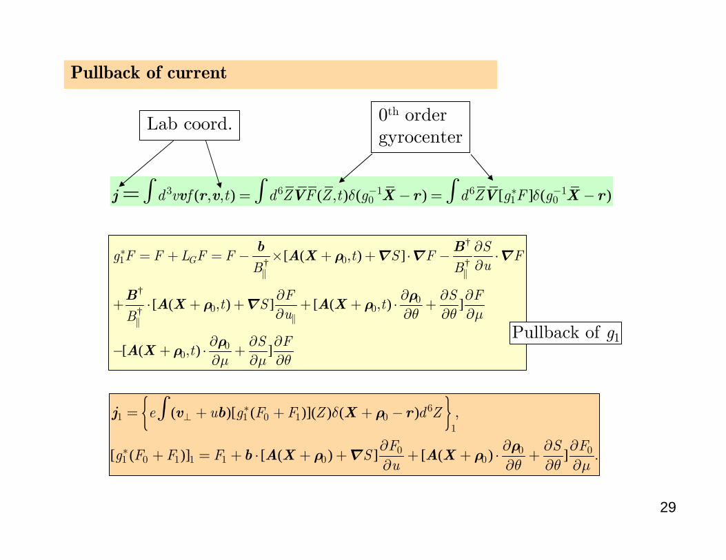
( ) ( ) ( ) [ ] ( )3 6 1 6 10 1 0d v f t d Z F Z t g d Z g F gδ δ− ∗ −, , = , − = −= ∫ ∫ ∫j v r v V X r V X r
†
† †
†
†
[ ( ) ]
[ ( ) ] [ ( ) ]
[ ( ) ]
1 0
00 0
00
GS
g F F L F F t S F FuB B
F S Ft S t
uB
S Ft
θ θ µ
µ µ θ
∗ ∂= + = − × + , + ⋅ − ⋅
∂
∂ ∂ ∂ ∂+ ⋅ + , + + + , ⋅ +
∂ ∂ ∂ ∂
∂ ∂ ∂− + , ⋅ +
∂ ∂ ∂
b BA X
BA X A X
A X
ρ ∇ ∇ ∇
ρρ ∇ ρ
ρρ
( )[ ( )]( ) ( )
[ ( )] [ ( ) ] [ ( ) ]
61 1 0 1 0
1
0 0 01 0 1 1 1 0 0
e u g F F Z d Z
F S Fg F F F S
u
δ
θ θ µ
∗⊥
∗
= ,+ + + −
∂ ∂ ∂ ∂+ = + ⋅ + + + + ⋅ + .
∂ ∂ ∂ ∂
∫j v b X r
b A X A X
ρ
ρρ ∇ ρ
Pullback of current
Lab coord. 0th order gyrocenter
1Pullback of g
30
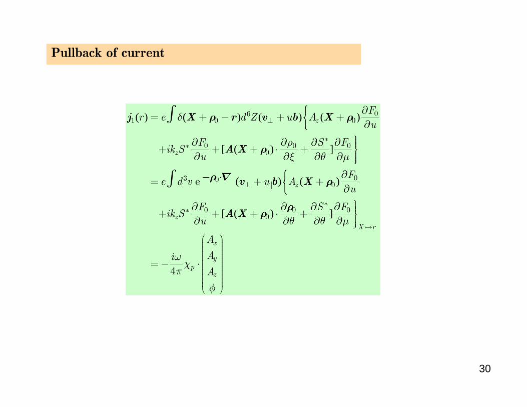
( ) ( ) ( ) ( )
[ ( ) ]
( ) ( )
[ ( ) ]
061 0 0
0 0 00
03 00
0 0 00
e
4
z
z
z
zX r
x
yp
z
Fr e d Z u A
u
F S Fik S
u
Fe d v u A
u
F S Fik S
u
A
AiA
δ
ρξ θ µ
θ θ µ
ωχ
π
φ
⊥
∗∗
⊥
∗∗
∂= + − + +
∂⎫∂ ∂ ∂ ∂ ⎪⎪+ + + ⋅ + ⎬⎪∂ ∂ ∂ ∂ ⎪⎭
∂− ⋅= + +∂⎫∂ ∂ ∂ ∂ ⎪⎪+ + + ⋅ + ⎬⎪∂ ∂ ∂ ∂ ⎪⎭
⎛ ⎞⎟⎜ ⎟⎜ ⎟⎜ ⎟⎜=− ⋅⎜⎜⎜⎜⎜⎜⎝ ⎠
∫
∫
j X r v b X
A X
v b X
A X
ρ ρ
ρ
ρ ∇ ρ
ρρ
⎟⎟⎟⎟⎟⎟⎟
Pullback of current
31
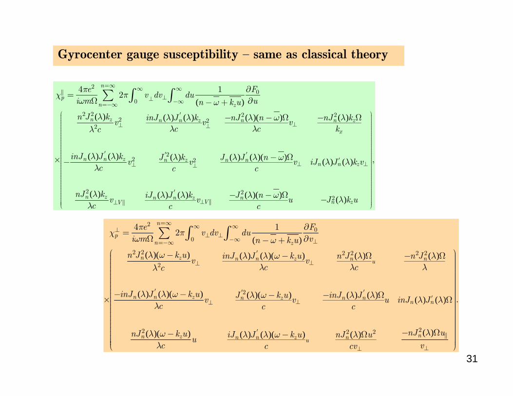
( )
( ) ( ) ( ) ( )( ) ( )
( ) ( ) ( ) ( ) ( )( ) ( ) ( )
( )
20
0
2 2 2 22 2
2
22 2
2
4 12
n
pn z
n z n n z n n z
x
n n z n z n nn n z
n z
e Fv dv du
i m un k u
n J k inJ J k nJ n nJ kv v vc c kc
inJ J k J k J J nv v v iJ J k vc c c
nJ kc
πχ π
ω ω
λ λ λ λ ω λλ λλ
λ λ λ λ λ ω λ λλ
λλ
=∞ ∞ ∞⊥⊥ −∞=−∞
′
⊥⊥ ⊥
′ ′ ′′
⊥ ⊥⊥ ⊥
∂=
Ω ∂− +
− − Ω − Ω
− Ω× −
∑ ∫ ∫
( ) ( ) ( )( ) ( )2
2n n z nV n zV
iJ J k J nv v u J k uc c
λ λ λ ω λ
⎛ ⎞⎟⎜ ⎟⎜ ⎟⎜ ⎟⎜ ⎟⎜ ⎟⎜ ⎟⎜ ⎟⎟⎜ ⎟⎜ ⎟⎜ ⎟⎜ ⎟⎜ ⎟⎜ ⎟⎜ ⎟⎜ ⎟⎟⎜ ⎟⎜ ⎟⎜ ⎟⎜ ⎟⎜ ⎟⎜ ⎟⎜ ⎟⎜ ⎟⎟⎜ ⎟⎜ ⎟⎜ ⎟⎜ ⎟⎜ ⎟⎜ ⎟⎜ ⎟′⎜ ⎟⎜ ⎟⎟⎜ ⎟⎜ ⊥ ⎟⊥⎜ ⎟⎜⎝ ⎠
,
− − Ω −
( )
( )( ) ( ) ( )( ) ( ) ( )
( ) ( )( ) ( )( ) ( ) ( ) ( ) ( )
( )
20
0
2 2 2 2 2 2
2
2
2
4 12
n
pn z
n z n n z n nu
n n z n z n nn n
n
e Fv dv du
i m vn k u
n J k u inJ J k u n J n Jv vc cc
inJ J k u J k u inJ Jv v u inJ Jc c c
nJ
πχ π
ω ω
λ ω λ λ ω λ λλ λ λλ
λ λ ω λ ω λ λ λ λλ
λ
=∞ ∞ ∞⊥⊥ ⊥
−∞ ⊥=−∞
′
⊥⊥
′ ′ ′′
⊥⊥
∂=
Ω ∂− +
− − Ω − Ω
− − − − Ω× Ω
∑ ∫ ∫
( )( ) ( ) ( )( ) ( ) 22 2 nz n n z nunJ uk u iJ J k u nJ uu
c vc cv
λω λ λ ω λλ
′
⊥⊥
⎛ ⎞⎟⎜ ⎟⎜ ⎟⎜ ⎟⎜ ⎟⎜ ⎟⎜ ⎟⎜ ⎟⎟⎜ ⎟⎜ ⎟⎜ ⎟⎜ ⎟.⎜ ⎟⎜ ⎟⎜ ⎟⎜ ⎟⎟⎜ ⎟⎜ ⎟⎜ ⎟⎜ ⎟⎜ ⎟− Ω−⎜ − Ω ⎟⎜ ⎟⎜ ⎟⎟⎜⎝ ⎠
Gyrocenter gauge susceptibility – same as classical theory
32
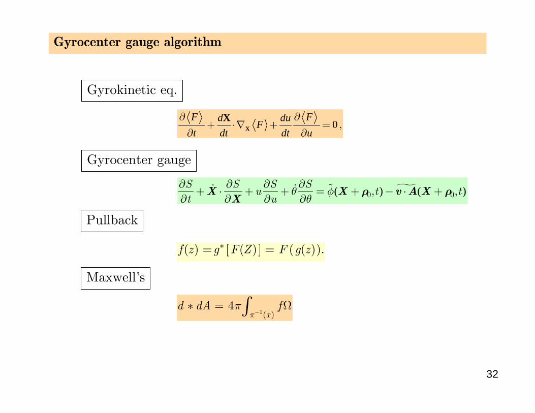
Gyrocenter gauge algorithm
0∂ ∂
+ ⋅∇ + = ,∂ ∂
F Fd duFt dt dt uX
X
( ) ( )0 0S S S S
u t tt u
θ φθ
∂ ∂ ∂ ∂+ ⋅ + + = + , − ⋅ + ,
∂ ∂ ∂ ∂X X v A X
Xρ ρ
[ ] ( )( ) ( ) ( )f z g F Z F g z∗= = .
1( )4
xd dA f
ππ
−∗ = Ω∫
Gyrokinetic eq.
Gyrocenter gauge
Pullback
Maxwell’s
33
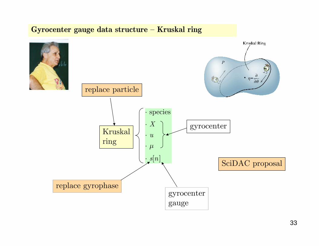
Gyrocenter gauge data structure – Kruskal ring
Kruskalring
gyrocentergauge
species
[ ]
X
u
s n
µ
⋅
⋅⋅⋅
⋅
gyrocenter
replace gyrophase
replace particle
SciDAC proposal
34
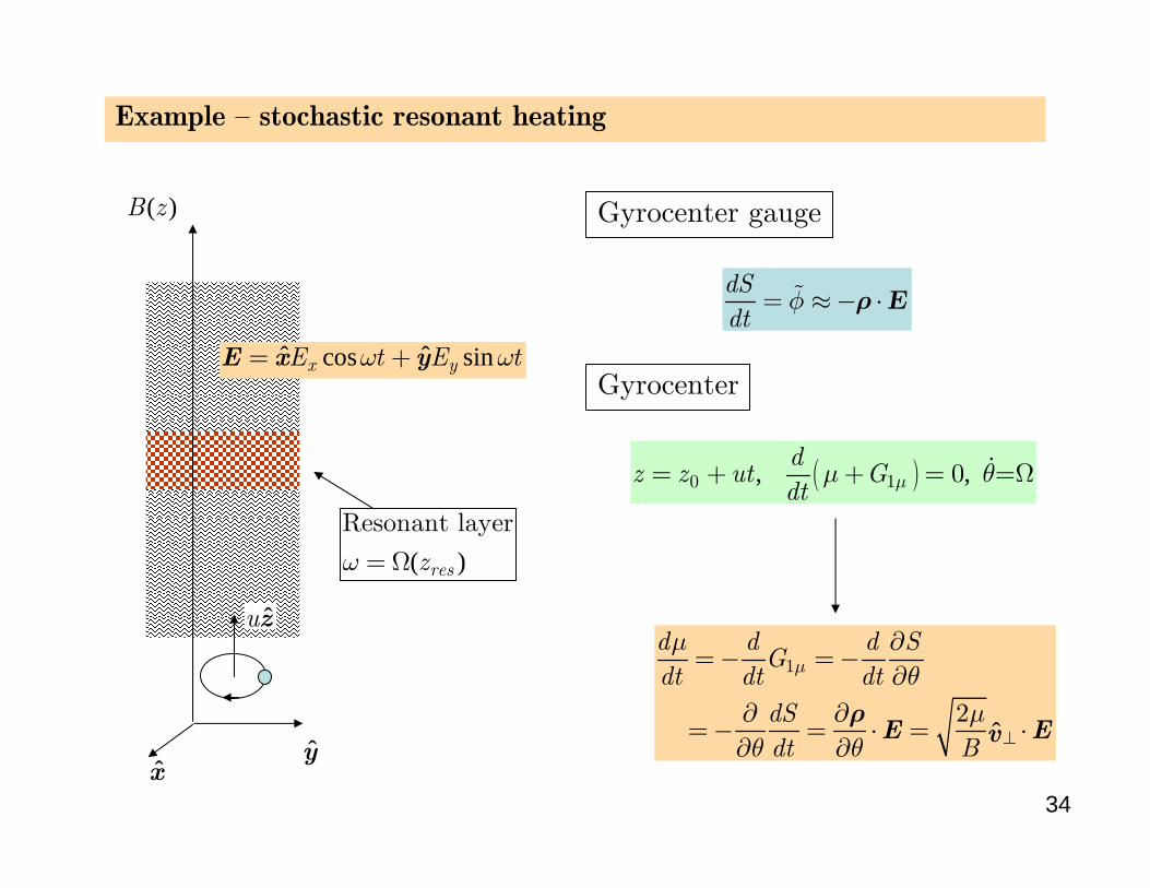
( ), ,0 1 0 =d
z z ut Gdt µµ θ= + + = Ω
Example – stochastic resonant heating
( )B z
ˆ ˆcos sinx yE t E tω ω= +E x y
dSdt
φ= ≈− ⋅ρ Ε
xy
( )Resonant layer
reszω =Ω
Gyrocenter gauge
Gyrocenter
ˆuz
ˆ
1
2
d d d SG
dt dt dtdSdt B
µµ
θµ
θ θ ⊥
∂=− =−
∂∂ ∂
=− = ⋅ = ⋅∂ ∂
E Evρ
35
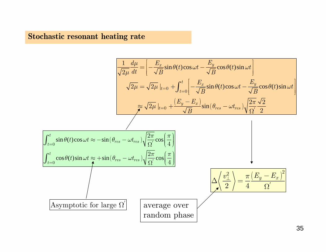
( )( )
sin ( )cos cos ( )sin
sin ( )cos cos ( )sin
sin
00
0
12
2 2
2 22
2
yx
t yxt
t
y xt res res
Ed Et t t t
dt B B
EEt t t t
B B
E Et
B
µθ ω θ ω
µ
µ µ θ ω θ ω
πµ θ ω
==
= ′
⎡ ⎤⎢ ⎥= − −⎢ ⎥⎣ ⎦
⎡ ⎤⎢ ⎥= | + − −⎢ ⎥⎣ ⎦
−≈ | + −
Ω
∫
( )
( )
sin ( )cos sin cos
cos ( )sin sin cos
0
0
24
24
t
res rest
t
res rest
t t t
t t t
π πθ ω θ ω
π πθ ω θ ω
′=
′=
⎛ ⎞⎟⎜≈− − ⎟⎜ ⎟⎜⎝ ⎠Ω⎛ ⎞⎟⎜≈ + − ⎟⎜ ⎟⎜⎝ ⎠Ω
∫
∫
( )22
2 4y xE Ev π⊥
′
−∆ =
Ω
Asymptotic for large ′Ω average overrandom phase
Stochastic resonant heating rate
36
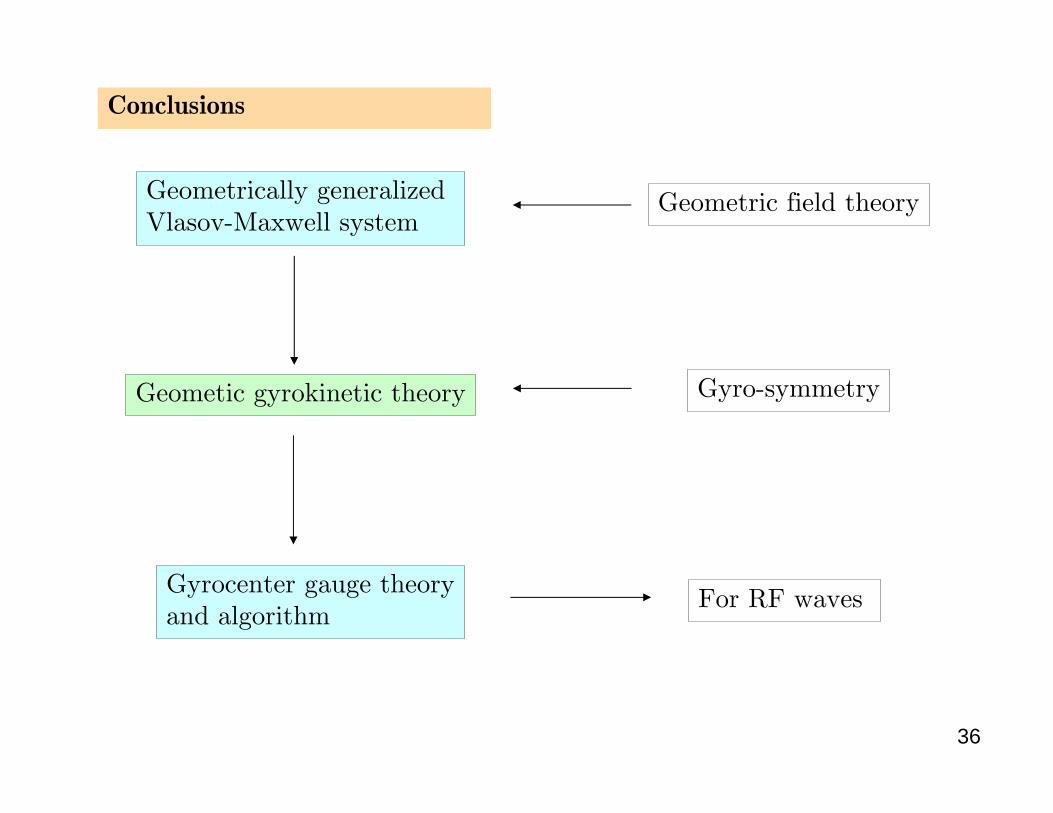
Conclusions
Geometrically generalized Vlasov-Maxwell system
Geometic gyrokinetic theory
Gyrocenter gauge theoryand algorithm
Geometric field theory
Gyro-symmetry
For RF waves