gauge theories and the gauge argument - …publish.uwo.ca/~csmeenk2/files/gaugeargument.pdfgauge...
TRANSCRIPT
Gauge Theories and the Gauge Argument
Gauge Theories and the Gauge Argument
Robert Moir
The University of Western OntarioDept. of Philosophy
February 5, 2009
Gauge Theories and the Gauge Argument
Table of Contents
1 Gauge Theories
2 Classical Electromagnetism
3 Lagrangian Mechanics of FieldsLagrangian Mechanics of Point ParticlesLagrangian Mechanics of FieldsRelativistic Field Theories
4 The Gauge Argument for a Complex Scalar Field
5 Yang-Mills Theory
Gauge Theories and the Gauge Argument
Gauge Theories
1 Gauge Theories
2 Classical Electromagnetism
3 Lagrangian Mechanics of FieldsLagrangian Mechanics of Point ParticlesLagrangian Mechanics of FieldsRelativistic Field Theories
4 The Gauge Argument for a Complex Scalar Field
5 Yang-Mills Theory
Gauge Theories and the Gauge Argument
Gauge Theories
Gauge Theories
The Fundamental Theories of Contemporary Physics
General Relativity — Classical Field Theory (Gravity)
Standard Model — Quantum Field Theories
Quantum Chromodynamics (QCD) (Strong Force)GWS Electroweak Theory (EWT) (Weak and EM Forces)
Gauge Theories and the Gauge Argument
Gauge Theories
Gauge Theories
The Fundamental Theories of Contemporary Physics
General Relativity — Classical Field Theory (Gravity)
Standard Model — Quantum Field Theories
Quantum Chromodynamics (QCD) (Strong Force)
GWS Electroweak Theory (EWT) (Weak and EM Forces)
Gauge Theories and the Gauge Argument
Gauge Theories
Gauge Theories
The Fundamental Theories of Contemporary Physics
General Relativity — Classical Field Theory (Gravity)
Standard Model — Quantum Field Theories
Quantum Chromodynamics (QCD) (Strong Force)GWS Electroweak Theory (EWT) (Weak and EM Forces)
Gauge Theories and the Gauge Argument
Gauge Theories
Field Quantization of Classical Fields
The quantum field theories of the Standard Model areobtained by ‘quantizing’ classical field theories.
It is sometimes claimed that these classical field theories canbe ‘derived’ using a kind of argument called a gaugeargument.
Gauge Theories and the Gauge Argument
Gauge Theories
Gauge Arguments
The Lagrangians of the classical field theories are invariantunder a group of transformations of the field.
Such a symmetry (invariance) is called a global symmetry,since the transformation of the field that leaves theLagrangian invariant does not depend on the location in spaceor spacetime.
The gauge argument proceeds by making the Lagrangianinvariant under ‘local’ transformations of the field, local in thesense of depending on the location in space or spacetime (onwhich the field is defined).
Gauge Theories and the Gauge Argument
Gauge Theories
Gauge Transformations
The transformations of the fields in gauge arguments do notchange the physical state of the field, they are transformationsin an ‘internal space’ of the field, in a sense to be describedlater.
Consequently, more than one field state in this internal spacedescribes the same physical field.
The different states that are physically equivalent are looselyanalogous to the arbitrary choice of gauge in the sense of anarbitrary choice of ‘length’ scale, e.g. feet or metres, secondsor years, kelvin or rankine, etc.
Consequently, the transformations leaving the Lagrangianinvariant are called gauge transformations.
Gauge Theories and the Gauge Argument
Gauge Theories
Gauge Arguments
A gauge argument starts with a Lorentz covariant Lagrangianof a classical field that is invariant under a global gaugetransformation, or gauge transformation of the first kind.
An attempt is then made to make the Lagrangian invariantunder the same kind of transformation that varies dependingon the spacetime location, i.e. a local gauge transformation,or gauge transformation of the second kind.
The initial Lagrangian is not invariant under a local gaugetransformation and the the gauge transformed Lagrangianceases to be Lorentz covariant.
Terms are introduced to restore Lorentz and local gaugeinvariance, which introduces one or more vector fields Aµ(xν).
Then allowing Aµ to contribute directly to the Lagrangianintroduces a gauge field tensor Fµν for each Aµ.
Gauge Theories and the Gauge Argument
Gauge Theories
Gauge Arguments
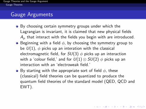
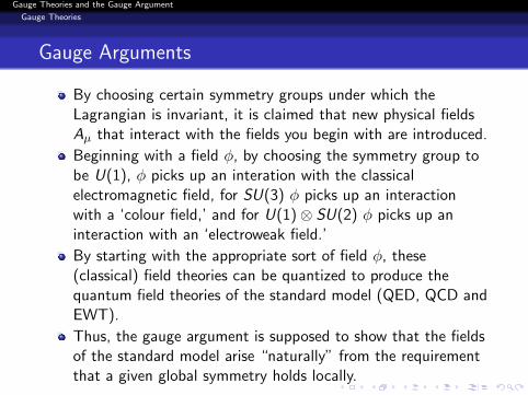
By choosing certain symmetry groups under which theLagrangian is invariant, it is claimed that new physical fieldsAµ that interact with the fields you begin with are introduced.
Beginning with a field φ, by choosing the symmetry group tobe U(1), φ picks up an interation with the classicalelectromagnetic field, for SU(3) φ picks up an interactionwith a ‘colour field,’ and for U(1)⊗ SU(2) φ picks up aninteraction with an ‘electroweak field.’
By starting with the appropriate sort of field φ, these(classical) field theories can be quantized to produce thequantum field theories of the standard model (QED, QCD andEWT).
Thus, the gauge argument is supposed to show that the fieldsof the standard model arise “naturally” from the requirementthat a given global symmetry holds locally.
Gauge Theories and the Gauge Argument
Gauge Theories
Gauge Arguments
By choosing certain symmetry groups under which theLagrangian is invariant, it is claimed that new physical fieldsAµ that interact with the fields you begin with are introduced.
Beginning with a field φ, by choosing the symmetry group tobe U(1), φ picks up an interation with the classicalelectromagnetic field, for SU(3) φ picks up an interactionwith a ‘colour field,’ and for U(1)⊗ SU(2) φ picks up aninteraction with an ‘electroweak field.’
By starting with the appropriate sort of field φ, these(classical) field theories can be quantized to produce thequantum field theories of the standard model (QED, QCD andEWT).
Thus, the gauge argument is supposed to show that the fieldsof the standard model arise “naturally” from the requirementthat a given global symmetry holds locally.
Gauge Theories and the Gauge Argument
Classical Electromagnetism
1 Gauge Theories
2 Classical Electromagnetism
3 Lagrangian Mechanics of FieldsLagrangian Mechanics of Point ParticlesLagrangian Mechanics of FieldsRelativistic Field Theories
4 The Gauge Argument for a Complex Scalar Field
5 Yang-Mills Theory
Gauge Theories and the Gauge Argument
Classical Electromagnetism
Charges and Currents
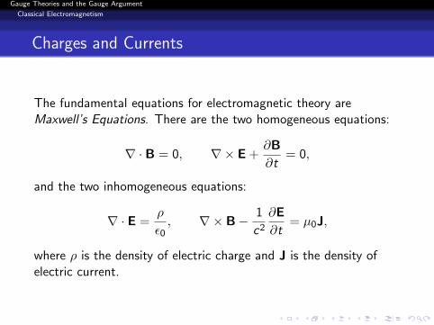
The fundamental equations for electromagnetic theory areMaxwell’s Equations. There are the two homogeneous equations:
∇ · B = 0, ∇× E +∂B
∂t= 0,
and the two inhomogeneous equations:
∇ · E =ρ
ε0, ∇× B− 1
c2
∂E
∂t= µ0J,
where ρ is the density of electric charge and J is the density ofelectric current.
Gauge Theories and the Gauge Argument
Classical Electromagnetism
Potentials
Since ∇ · B = 0 and for any vector field f, ∇ · (∇× f) = 0, themagnetic field can be defined in terms of a vector potential A,such that
B = ∇× A.
This enables the other homogeneous Maxwell equation to bewritten as
∇×(
E +∂A
∂t
)= 0.
Then, since for any scalar field f , ∇× (∇f ) = 0, the quantityabove with the vanishing curl can be written in terms of a scalarpotential ϕ, such that
E +∂A
∂t= −∇ϕ.
Gauge Theories and the Gauge Argument
Classical Electromagnetism
Potentials
Thus, we can write the electric and magnetic fields, E and B, interms of a vector and scalar potential, A and ϕ, as
B = ∇× A, E = −∇ϕ− ∂A
∂t.
Gauge Theories and the Gauge Argument
Classical Electromagnetism
Gauge Freedom
Since the magnetic field is defined as the curl of the vectorpotential A, the gradient of any scalar field Λ can be added to Awithout changing the magnetic field.
Thus, the transformation
A −→ A′ = A−∇Λ
leaves the magnetic field invariant. So by describing the magneticfield in terms of a potential a descriptive freedom is introduced,since there is no unique vector potential that determines themagnetic field.
This descriptive freedom is called gauge freedom and thetransformation of the potential leaving the field invariant is calleda gauge transformation.
Gauge Theories and the Gauge Argument
Classical Electromagnetism
Gauge Transformations
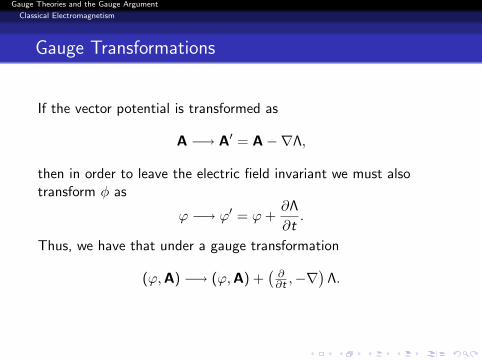
If the vector potential is transformed as
A −→ A′ = A−∇Λ,
then in order to leave the electric field invariant we must alsotransform φ as
ϕ −→ ϕ′ = ϕ+∂Λ
∂t.
Thus, we have that under a gauge transformation
(ϕ,A) −→ (ϕ,A) +(∂∂t ,−∇
)Λ.
Gauge Theories and the Gauge Argument
Classical Electromagnetism
Gauge Transformations
If the vector potential is transformed as
A −→ A′ = A−∇Λ,
then in order to leave the electric field invariant we must alsotransform φ as
ϕ −→ ϕ′ = ϕ+∂Λ
∂t.
Thus, we have that under a gauge transformation
(ϕ,A) −→ (ϕ,A) +(∂∂t ,−∇
)Λ.
Gauge Theories and the Gauge Argument
Classical Electromagnetism
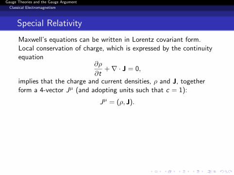
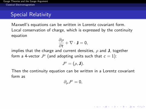
Special Relativity
Maxwell’s equations can be written in Lorentz covariant form.Local conservation of charge, which is expressed by the continuityequation
∂ρ
∂t+∇ · J = 0,
implies that the charge and current densities, ρ and J, togetherform a 4-vector Jµ (and adopting units such that c = 1):
Jµ = (ρ, J).
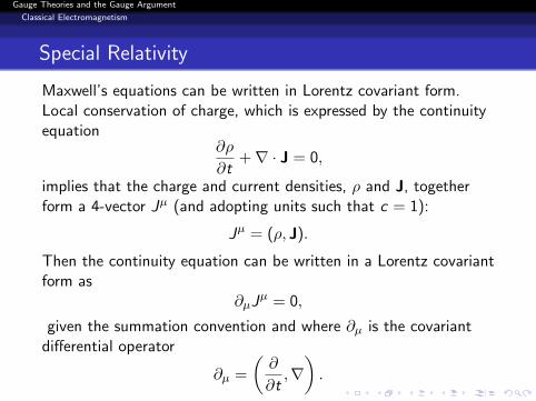
Then the continuity equation can be written in a Lorentz covariantform as
∂µJµ = 0,
given the summation convention and where ∂µ is the covariantdifferential operator
∂µ =
(∂
∂t,∇).
Gauge Theories and the Gauge Argument
Classical Electromagnetism
Special Relativity
Maxwell’s equations can be written in Lorentz covariant form.Local conservation of charge, which is expressed by the continuityequation
∂ρ
∂t+∇ · J = 0,
implies that the charge and current densities, ρ and J, togetherform a 4-vector Jµ (and adopting units such that c = 1):
Jµ = (ρ, J).
Then the continuity equation can be written in a Lorentz covariantform as
∂µJµ = 0,
given the summation convention and where ∂µ is the covariantdifferential operator
∂µ =
(∂
∂t,∇).
Gauge Theories and the Gauge Argument
Classical Electromagnetism
Potentials Form a 4-vector
It can be shown that the scalar and vector potentials, ϕ and A,together form a contravariant 4-vector
Aµ = (ϕ,A).
Maxwell’s equations can be written in a Lorentz covariant form interms of Aµ.
Thus, the gauge transformation
(ϕ,A) −→ (ϕ,A) +(∂∂t ,−∇
)Λ
can be written asAµ −→ Aµ + ∂µΛ,
where ∂µ =(∂∂t ,−∇
)is the contravariant differential operator.
Gauge Theories and the Gauge Argument
Classical Electromagnetism
Lorentz Covariant Maxwell’s Equations
Given the expressions for E and B in terms of the scalar and vectorpotentials above, the various components of the fields can beexpressed in terms of the components of Aµ.
For example, we havefor the x components that
Ex = −∂Ax
∂t− ∂ϕ
∂x= −(∂0A1 − ∂1A0),
Bx =∂Az
∂y− ∂Ay
∂z= −(∂2A3 − ∂3A2),
given Aµ = (ϕ,A) and ∂µ =(∂∂t ,−∇
).
Gauge Theories and the Gauge Argument
Classical Electromagnetism
Lorentz Covariant Maxwell’s Equations
Given the expressions for E and B in terms of the scalar and vectorpotentials above, the various components of the fields can beexpressed in terms of the components of Aµ. For example, we havefor the x components that
Ex = −∂Ax
∂t− ∂ϕ
∂x= −(∂0A1 − ∂1A0),
Bx =∂Az
∂y− ∂Ay
∂z= −(∂2A3 − ∂3A2),
given Aµ = (ϕ,A) and ∂µ =(∂∂t ,−∇
).
Gauge Theories and the Gauge Argument
Classical Electromagnetism
Lorentz Covariant Maxwell’s Equations
The six equations for the six components of E and B determine asecond rank, antisymmetric field strength tensor
Fµν = ∂µAν − ∂νAµ.
Maxwell’s equations can be written in Lorentz covariant form interms of Fµν .
Gauge Theories and the Gauge Argument
Classical Electromagnetism
Lorentz Covariant Maxwell’s Equations
The two inhomogeneous Maxwell equations can be written as
∂µFµν = Jν ,
with Jν = (ρ, J) the 4-current.
Gauge Theories and the Gauge Argument
Classical Electromagnetism
Lorentz Covariant Maxwell’s Equations
The two homogeneous Maxwell equations can be written as thefour equations
∂λFµν + ∂µFνλ + ∂νFλµ = 0.
Gauge Theories and the Gauge Argument
Lagrangian Mechanics of Fields
1 Gauge Theories
2 Classical Electromagnetism
3 Lagrangian Mechanics of FieldsLagrangian Mechanics of Point ParticlesLagrangian Mechanics of FieldsRelativistic Field Theories
4 The Gauge Argument for a Complex Scalar Field
5 Yang-Mills Theory
Gauge Theories and the Gauge Argument
Lagrangian Mechanics of Fields
Lagrangian Mechanics of Point Particles
Lagrangian Formulation of Mechanics
The Lagrangian formulation of mechanics characterizes somephysical system in terms of independent generalized coordinates qi
and their time derivatives qi .
The number of independent coordinates is determined by thenumber of degrees of freedom of the system.
For example, an ideal pendulum has one degree of freedom andcan be described in terms of the angle θ that the string makes withthe equilibrium position of the string (vertical) and its timederivative θ.
The Lagrangian L(qi , qi , t) = T − V , where T is the kineticenergy and V the potential energy of the system.
Gauge Theories and the Gauge Argument
Lagrangian Mechanics of Fields
Lagrangian Mechanics of Point Particles
Lagrangian Formulation of Mechanics
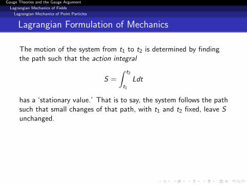
The motion of the system from t1 to t2 is determined by findingthe path such that the action integral
S =
∫ t2
t1
Ldt
has a ‘stationary value.’
That is to say, the system follows the pathsuch that small changes of that path, with t1 and t2 fixed, leave Sunchanged. This can be expressed by saying that the motion issuch that the variation of the action integral for fixed t1 and t2 is0, i.e.
δS = δ
∫ t2
t1
L(qi , qi , t)dt = 0.
This is called Hamilton’s Principle.
Gauge Theories and the Gauge Argument
Lagrangian Mechanics of Fields
Lagrangian Mechanics of Point Particles
Lagrangian Formulation of Mechanics
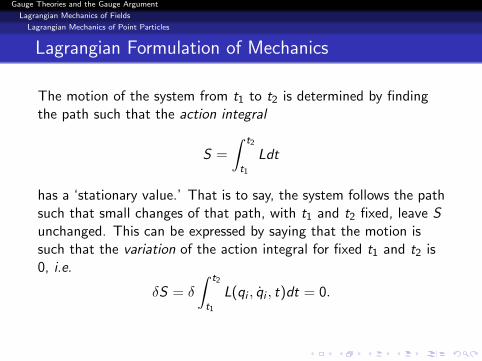
The motion of the system from t1 to t2 is determined by findingthe path such that the action integral
S =
∫ t2
t1
Ldt
has a ‘stationary value.’ That is to say, the system follows the pathsuch that small changes of that path, with t1 and t2 fixed, leave Sunchanged.
This can be expressed by saying that the motion issuch that the variation of the action integral for fixed t1 and t2 is0, i.e.
δS = δ
∫ t2
t1
L(qi , qi , t)dt = 0.
This is called Hamilton’s Principle.
Gauge Theories and the Gauge Argument
Lagrangian Mechanics of Fields
Lagrangian Mechanics of Point Particles
Lagrangian Formulation of Mechanics
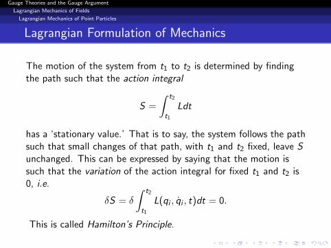
The motion of the system from t1 to t2 is determined by findingthe path such that the action integral
S =
∫ t2
t1
Ldt
has a ‘stationary value.’ That is to say, the system follows the pathsuch that small changes of that path, with t1 and t2 fixed, leave Sunchanged. This can be expressed by saying that the motion issuch that the variation of the action integral for fixed t1 and t2 is0, i.e.
δS = δ
∫ t2
t1
L(qi , qi , t)dt = 0.
This is called Hamilton’s Principle.
Gauge Theories and the Gauge Argument
Lagrangian Mechanics of Fields
Lagrangian Mechanics of Point Particles
Lagrangian Formulation of Mechanics
The motion of the system from t1 to t2 is determined by findingthe path such that the action integral
S =
∫ t2
t1
Ldt
has a ‘stationary value.’ That is to say, the system follows the pathsuch that small changes of that path, with t1 and t2 fixed, leave Sunchanged. This can be expressed by saying that the motion issuch that the variation of the action integral for fixed t1 and t2 is0, i.e.
δS = δ
∫ t2
t1
L(qi , qi , t)dt = 0.
This is called Hamilton’s Principle.
Gauge Theories and the Gauge Argument
Lagrangian Mechanics of Fields
Lagrangian Mechanics of Point Particles
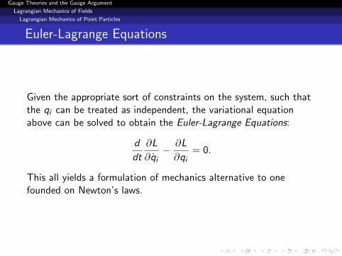
Euler-Lagrange Equations
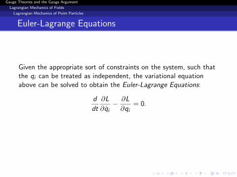
Given the appropriate sort of constraints on the system, such thatthe qi can be treated as independent, the variational equationabove can be solved to obtain the Euler-Lagrange Equations:
d
dt
∂L
∂qi− ∂L
∂qi= 0.
This all yields a formulation of mechanics alternative to onefounded on Newton’s laws.
Gauge Theories and the Gauge Argument
Lagrangian Mechanics of Fields
Lagrangian Mechanics of Point Particles
Euler-Lagrange Equations
Given the appropriate sort of constraints on the system, such thatthe qi can be treated as independent, the variational equationabove can be solved to obtain the Euler-Lagrange Equations:
d
dt
∂L
∂qi− ∂L
∂qi= 0.
This all yields a formulation of mechanics alternative to onefounded on Newton’s laws.
Gauge Theories and the Gauge Argument
Lagrangian Mechanics of Fields
Lagrangian Mechanics of Point Particles
Symmetry and Lagrangian Mechanics
If the Lagrangian is invariant under transformations of one or moreof the generalized coordinates qi , then the system has one or moreconserved quantities. This connection is established by Noether’stheorem. Thus, symmetries of the Lagrangian give rise toconserved quantities.
Gauge Theories and the Gauge Argument
Lagrangian Mechanics of Fields
Lagrangian Mechanics of Point Particles
Symmetry and Lagrangian Mechanics
To see how this works, suppose that L(qi , qi , t) does not dependon qk . Then
∂L
∂qk= 0.
Thus, the Euler-Lagrange equation for i = k reduces to
d
dt
∂L
∂qk= 0.
Gauge Theories and the Gauge Argument
Lagrangian Mechanics of Fields
Lagrangian Mechanics of Point Particles
Symmetry and Lagrangian Mechanics
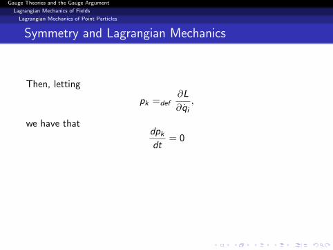
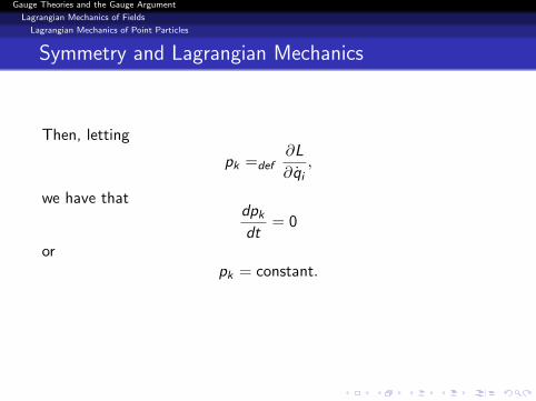
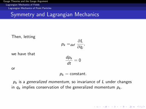
Then, letting
pk =def∂L
∂qi,
we have thatdpk
dt= 0
orpk = constant.
pk is a generalized momentum, so invariance of L under changesin qk implies conservation of the generalized momentum pk .
Gauge Theories and the Gauge Argument
Lagrangian Mechanics of Fields
Lagrangian Mechanics of Point Particles
Symmetry and Lagrangian Mechanics
Then, letting
pk =def∂L
∂qi,
we have thatdpk
dt= 0
orpk = constant.
pk is a generalized momentum, so invariance of L under changesin qk implies conservation of the generalized momentum pk .
Gauge Theories and the Gauge Argument
Lagrangian Mechanics of Fields
Lagrangian Mechanics of Fields
Lagrangian Mechanics of Fields
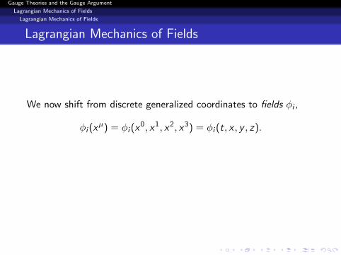
We now shift from discrete generalized coordinates to fields φi ,
φi (xµ) = φi (x0, x1, x2, x3) = φi (t, x , y , z).
The shift can be thought of as shifting from generalizedcoordinates qi (t) which are functions of time t, to fields φi (xµ),which are functions of spacetime location xµ.
Gauge Theories and the Gauge Argument
Lagrangian Mechanics of Fields
Lagrangian Mechanics of Fields
Lagrangian Mechanics of Fields
We shift from talking about a Lagrangian L to talking about aLagrangian density L(φi , ∂µφi ).
The equivalent of the Lagrangian isthe integral of L over all space:
L =
∫Ld3x .
Gauge Theories and the Gauge Argument
Lagrangian Mechanics of Fields
Lagrangian Mechanics of Fields
Lagrangian Mechanics of Fields
We shift from talking about a Lagrangian L to talking about aLagrangian density L(φi , ∂µφi ).The equivalent of the Lagrangian isthe integral of L over all space:
L =
∫Ld3x .
Gauge Theories and the Gauge Argument
Lagrangian Mechanics of Fields
Lagrangian Mechanics of Fields
Lagrangian Mechanics of Fields
The dynamics of the system are calculated by minimizing an actionintegral
S =
∫Ld4x .
Gauge Theories and the Gauge Argument
Lagrangian Mechanics of Fields
Lagrangian Mechanics of Fields
Lagrangian Mechanics of Fields
Consider now just a single field φ.
By determining the fieldconfiguration in some region R of spacetime such that thevariation δS of the action integral is zero when that the value ofthe field on the boundary of R is fixed, we obtain theEuler-Lagrange equations for the field:
∂
∂xµ
(∂L
∂(∂µφ)
)− ∂L∂φ
= 0.
Gauge Theories and the Gauge Argument
Lagrangian Mechanics of Fields
Lagrangian Mechanics of Fields
Lagrangian Mechanics of Fields
Consider now just a single field φ. By determining the fieldconfiguration in some region R of spacetime such that thevariation δS of the action integral is zero when that the value ofthe field on the boundary of R is fixed,
we obtain theEuler-Lagrange equations for the field:
∂
∂xµ
(∂L
∂(∂µφ)
)− ∂L∂φ
= 0.
Gauge Theories and the Gauge Argument
Lagrangian Mechanics of Fields
Lagrangian Mechanics of Fields
Lagrangian Mechanics of Fields
Consider now just a single field φ. By determining the fieldconfiguration in some region R of spacetime such that thevariation δS of the action integral is zero when that the value ofthe field on the boundary of R is fixed, we obtain theEuler-Lagrange equations for the field:
∂
∂xµ
(∂L
∂(∂µφ)
)− ∂L∂φ
= 0.
Gauge Theories and the Gauge Argument
Lagrangian Mechanics of Fields
Lagrangian Mechanics of Fields
Invariance of the Lagrangian Under Groups ofTransformations
Following a similar but more general argument that leads to theEuler-Lagrange equations for the field, and assuming that theLagrangian density L is invariant under some group oftransformations of xµ and φ, then it follows that there must be aconserved current Jµ, i.e. there is a Jµ such that
∂µJµ = 0.
This entails the existence of a conserved charge Q, which for sometime t = constant,
Q =
∫V
J0d3x ,
where V is a 3-volume in the spacelike hypersurface at time t.
Gauge Theories and the Gauge Argument
Lagrangian Mechanics of Fields
Lagrangian Mechanics of Fields
Invariance of the Lagrangian Under Groups ofTransformations
That the existence of a conserved current Jµ and charge Q isentailed by the invariance of the Lagrangian density under the (nothere specified) group of transformations is the content ofNoether’s theorem in the present context.
Invariance of the Lagrangian density under translation of the originof space and time lead to conservation of momentum and energy,respectively, and invariance under spatial rotations leads toconservation of angular momentum.
Gauge Theories and the Gauge Argument
Lagrangian Mechanics of Fields
Relativistic Field Theories
Klein-Gordon Equation
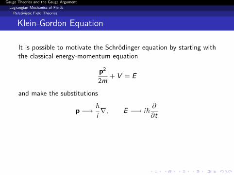
It is possible to motivate the Schrodinger equation by starting withthe classical energy-momentum equation
p2
2m+ V = E
and make the substitutions
p −→ ~i∇, E −→ i~
∂
∂t
to give (− ~2
2m∇2 + V
)ψ = i~
∂ψ
∂t
by letting the operators act on a wave function ψ.
Gauge Theories and the Gauge Argument
Lagrangian Mechanics of Fields
Relativistic Field Theories
Klein-Gordon Equation
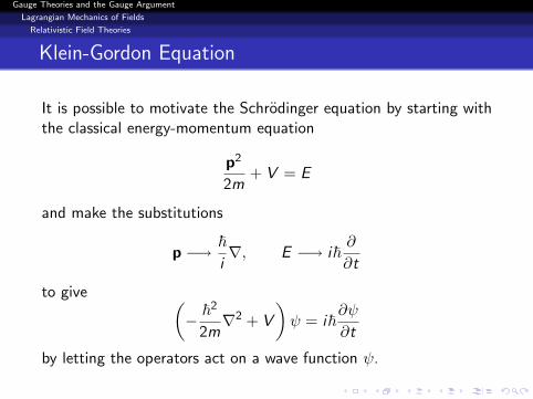
It is possible to motivate the Schrodinger equation by starting withthe classical energy-momentum equation
p2
2m+ V = E
and make the substitutions
p −→ ~i∇, E −→ i~
∂
∂t
to give (− ~2
2m∇2 + V
)ψ = i~
∂ψ
∂t
by letting the operators act on a wave function ψ.
Gauge Theories and the Gauge Argument
Lagrangian Mechanics of Fields
Relativistic Field Theories
Klein-Gordon Equation
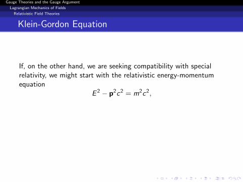
If, on the other hand, we are seeking compatibility with specialrelativity, we might start with the relativistic energy-momentumequation
E 2 − p2c2 = m2c2,
which in Lorentz covariant form is
pµpµ = m2c2.
Gauge Theories and the Gauge Argument
Lagrangian Mechanics of Fields
Relativistic Field Theories
Klein-Gordon Equation
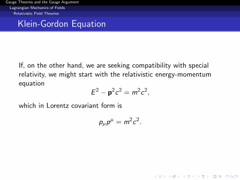
If, on the other hand, we are seeking compatibility with specialrelativity, we might start with the relativistic energy-momentumequation
E 2 − p2c2 = m2c2,
which in Lorentz covariant form is
pµpµ = m2c2.
Gauge Theories and the Gauge Argument
Lagrangian Mechanics of Fields
Relativistic Field Theories
Klein-Gordon Equation
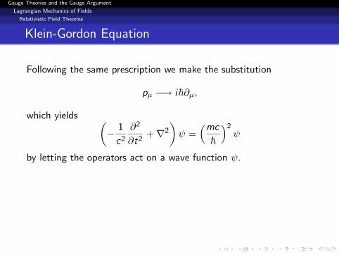
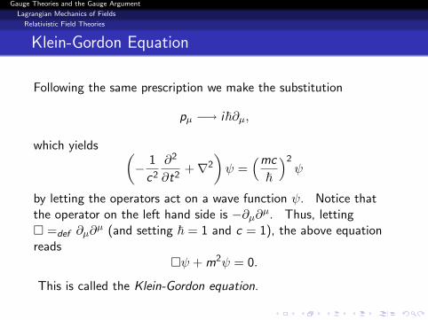
Following the same prescription we make the substitution
pµ −→ i~∂µ,
which yields (− 1
c2
∂2
∂t2+∇2
)ψ =
(mc
~
)2ψ
by letting the operators act on a wave function ψ. Notice thatthe operator on the left hand side is −∂µ∂µ. Thus, letting� =def ∂µ∂
µ (and setting ~ = 1 and c = 1), the above equationreads
�ψ + m2ψ = 0.
This is called the Klein-Gordon equation.
Gauge Theories and the Gauge Argument
Lagrangian Mechanics of Fields
Relativistic Field Theories
Klein-Gordon Equation
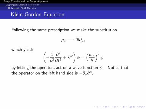
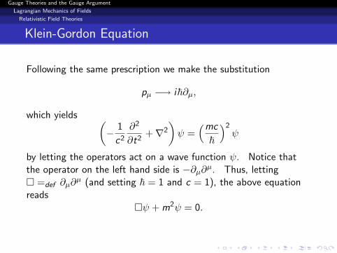
Following the same prescription we make the substitution
pµ −→ i~∂µ,
which yields (− 1
c2
∂2
∂t2+∇2
)ψ =
(mc
~
)2ψ
by letting the operators act on a wave function ψ.
Notice thatthe operator on the left hand side is −∂µ∂µ. Thus, letting� =def ∂µ∂
µ (and setting ~ = 1 and c = 1), the above equationreads
�ψ + m2ψ = 0.
This is called the Klein-Gordon equation.
Gauge Theories and the Gauge Argument
Lagrangian Mechanics of Fields
Relativistic Field Theories
Klein-Gordon Equation
Following the same prescription we make the substitution
pµ −→ i~∂µ,
which yields (− 1
c2
∂2
∂t2+∇2
)ψ =
(mc
~
)2ψ
by letting the operators act on a wave function ψ. Notice thatthe operator on the left hand side is −∂µ∂µ.
Thus, letting� =def ∂µ∂
µ (and setting ~ = 1 and c = 1), the above equationreads
�ψ + m2ψ = 0.
This is called the Klein-Gordon equation.
Gauge Theories and the Gauge Argument
Lagrangian Mechanics of Fields
Relativistic Field Theories
Klein-Gordon Equation
Following the same prescription we make the substitution
pµ −→ i~∂µ,
which yields (− 1
c2
∂2
∂t2+∇2
)ψ =
(mc
~
)2ψ
by letting the operators act on a wave function ψ. Notice thatthe operator on the left hand side is −∂µ∂µ. Thus, letting� =def ∂µ∂
µ (and setting ~ = 1 and c = 1), the above equationreads
�ψ + m2ψ = 0.
This is called the Klein-Gordon equation.
Gauge Theories and the Gauge Argument
Lagrangian Mechanics of Fields
Relativistic Field Theories
Klein-Gordon Equation
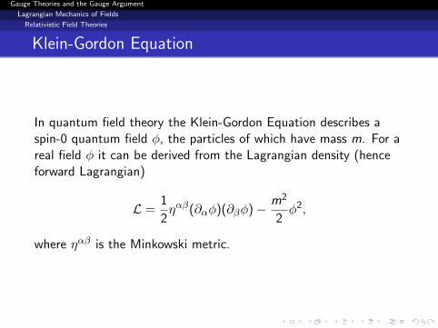
In quantum field theory the Klein-Gordon Equation describes aspin-0 quantum field φ, the particles of which have mass m.
For areal field φ it can be derived from the Lagrangian density (henceforward Lagrangian)
L =1
2ηαβ(∂αφ)(∂βφ)− m2
2φ2,
where ηαβ is the Minkowski metric.
Gauge Theories and the Gauge Argument
Lagrangian Mechanics of Fields
Relativistic Field Theories
Klein-Gordon Equation
In quantum field theory the Klein-Gordon Equation describes aspin-0 quantum field φ, the particles of which have mass m. For areal field φ it can be derived from the Lagrangian density (henceforward Lagrangian)
L =1
2ηαβ(∂αφ)(∂βφ)− m2
2φ2,
where ηαβ is the Minkowski metric.
Gauge Theories and the Gauge Argument
The Gauge Argument for a Complex Scalar Field
1 Gauge Theories
2 Classical Electromagnetism
3 Lagrangian Mechanics of FieldsLagrangian Mechanics of Point ParticlesLagrangian Mechanics of FieldsRelativistic Field Theories
4 The Gauge Argument for a Complex Scalar Field
5 Yang-Mills Theory
Gauge Theories and the Gauge Argument
The Gauge Argument for a Complex Scalar Field
An Example of A Gauge Argument
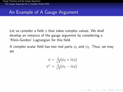
Let us consider a field φ that takes complex values. We shalldevelop an instance of the gauge argument by considering a‘Klein-Gordon’ Lagrangian for this field.
A complex scalar field has two real parts φ1 and φ2. Thus, we mayset
φ = 1√2
(φ1 + iφ2)
φ∗ = 1√2
(φ1 − iφ2)
Gauge Theories and the Gauge Argument
The Gauge Argument for a Complex Scalar Field
An Example of A Gauge Argument
Let us consider a field φ that takes complex values. We shalldevelop an instance of the gauge argument by considering a‘Klein-Gordon’ Lagrangian for this field.
A complex scalar field has two real parts φ1 and φ2. Thus, we mayset
φ = 1√2
(φ1 + iφ2)
φ∗ = 1√2
(φ1 − iφ2)
Gauge Theories and the Gauge Argument
The Gauge Argument for a Complex Scalar Field
Lagrangian for a Complex Scalar Field
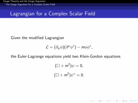
Given the modified Lagrangian
L = (∂µφ)(∂µφ∗)−mφφ∗,
the Euler-Lagrange equations yield two Klein-Gordon equations
(� + m2)ψ = 0,
(� + m2)ψ∗ = 0.
Gauge Theories and the Gauge Argument
The Gauge Argument for a Complex Scalar Field
‘Global’ Gauge Invariance
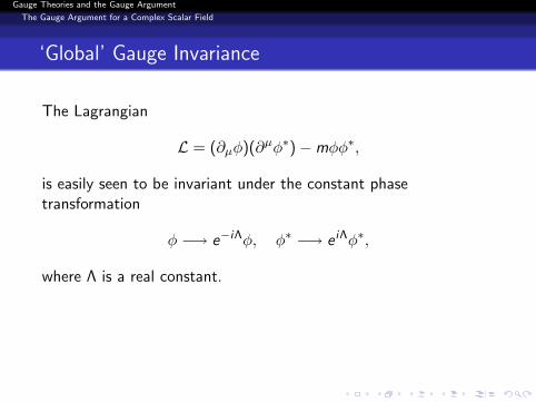
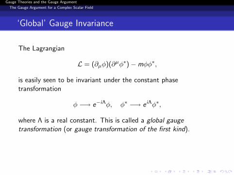
The Lagrangian
L = (∂µφ)(∂µφ∗)−mφφ∗,
is easily seen to be invariant under the constant phasetransformation
φ −→ e−iΛφ, φ∗ −→ e iΛφ∗,
where Λ is a real constant.
This is called a global gaugetransformation (or gauge transformation of the first kind). Theterm constant gauge transformation is perhaps more appropriate,constant since Λ is a constant (it does not depend on spacetimelocation).
Gauge Theories and the Gauge Argument
The Gauge Argument for a Complex Scalar Field
‘Global’ Gauge Invariance
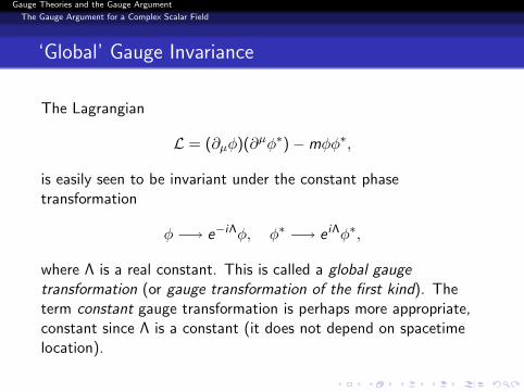
The Lagrangian
L = (∂µφ)(∂µφ∗)−mφφ∗,
is easily seen to be invariant under the constant phasetransformation
φ −→ e−iΛφ, φ∗ −→ e iΛφ∗,
where Λ is a real constant. This is called a global gaugetransformation (or gauge transformation of the first kind).
Theterm constant gauge transformation is perhaps more appropriate,constant since Λ is a constant (it does not depend on spacetimelocation).
Gauge Theories and the Gauge Argument
The Gauge Argument for a Complex Scalar Field
‘Global’ Gauge Invariance
The Lagrangian
L = (∂µφ)(∂µφ∗)−mφφ∗,
is easily seen to be invariant under the constant phasetransformation
φ −→ e−iΛφ, φ∗ −→ e iΛφ∗,
where Λ is a real constant. This is called a global gaugetransformation (or gauge transformation of the first kind). Theterm constant gauge transformation is perhaps more appropriate,constant since Λ is a constant (it does not depend on spacetimelocation).
Gauge Theories and the Gauge Argument
The Gauge Argument for a Complex Scalar Field
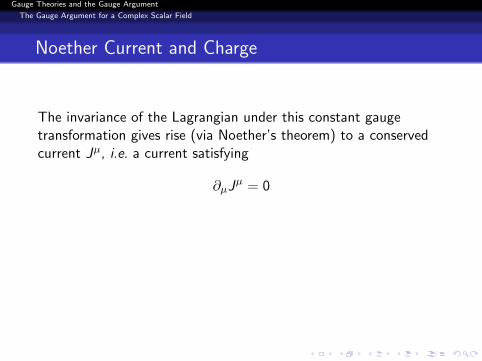
Noether Current and Charge
The invariance of the Lagrangian under this constant gaugetransformation gives rise (via Noether’s theorem) to a conservedcurrent Jµ, i.e. a current satisfying
∂µJµ = 0
and a conserved charge
Q =
∫V
J0dV ,
i.e. Q = constant.
Gauge Theories and the Gauge Argument
The Gauge Argument for a Complex Scalar Field
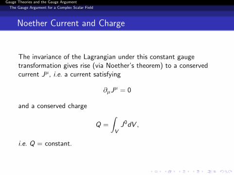
Noether Current and Charge
The invariance of the Lagrangian under this constant gaugetransformation gives rise (via Noether’s theorem) to a conservedcurrent Jµ, i.e. a current satisfying
∂µJµ = 0
and a conserved charge
Q =
∫V
J0dV ,
i.e. Q = constant.
Gauge Theories and the Gauge Argument
The Gauge Argument for a Complex Scalar Field
Gauge Transformation as an Internal Rotation
The constant gauge transformation described above can bethought of geometrically. Letting
~φ = φ1 i + φ2 j
the gauge transformation can be thought of as a rotation of thevector ~φ through an angle Λ.
The rotation is represented by the1× 1 complex matrix e iΛ. Since the Lagrangian is invariant underall such matrices, the Lagrangian is invariant under the group U(1).
Gauge Theories and the Gauge Argument
The Gauge Argument for a Complex Scalar Field
Gauge Transformation as an Internal Rotation
The constant gauge transformation described above can bethought of geometrically. Letting
~φ = φ1 i + φ2 j
the gauge transformation can be thought of as a rotation of thevector ~φ through an angle Λ. The rotation is represented by the1× 1 complex matrix e iΛ.
Since the Lagrangian is invariant underall such matrices, the Lagrangian is invariant under the group U(1).
Gauge Theories and the Gauge Argument
The Gauge Argument for a Complex Scalar Field
Gauge Transformation as an Internal Rotation
The constant gauge transformation described above can bethought of geometrically. Letting
~φ = φ1 i + φ2 j
the gauge transformation can be thought of as a rotation of thevector ~φ through an angle Λ. The rotation is represented by the1× 1 complex matrix e iΛ. Since the Lagrangian is invariant underall such matrices, the Lagrangian is invariant under the group U(1).
Gauge Theories and the Gauge Argument
The Gauge Argument for a Complex Scalar Field
Making the Gauge Symmetry ‘Local’
The next stage in the gauge argument is to make the ‘global’, orconstant, transformation ‘local’, or variable.
This is to say, anattempt is made to make the Lagrangian invariant under internalrotations e iΛ(xµ), where Λ is now a function of spacetime locationxµ (such a transformation is also called a gauge transformation ofthe second kind). Thought of geometrically, the vector
~φ(xµ) = φ(xµ)i + φ∗(xµ)j
is (in general) rotated by a different angle Λ(xµ) at each spacetimelocation xµ (and in such a way that the amount of rotationchanges smoothly from spacetime point to spacetime point).
Gauge Theories and the Gauge Argument
The Gauge Argument for a Complex Scalar Field
Making the Gauge Symmetry ‘Local’
The next stage in the gauge argument is to make the ‘global’, orconstant, transformation ‘local’, or variable. This is to say, anattempt is made to make the Lagrangian invariant under internalrotations e iΛ(xµ), where Λ is now a function of spacetime locationxµ (such a transformation is also called a gauge transformation ofthe second kind).
Thought of geometrically, the vector
~φ(xµ) = φ(xµ)i + φ∗(xµ)j
is (in general) rotated by a different angle Λ(xµ) at each spacetimelocation xµ (and in such a way that the amount of rotationchanges smoothly from spacetime point to spacetime point).
Gauge Theories and the Gauge Argument
The Gauge Argument for a Complex Scalar Field
Making the Gauge Symmetry ‘Local’
The next stage in the gauge argument is to make the ‘global’, orconstant, transformation ‘local’, or variable. This is to say, anattempt is made to make the Lagrangian invariant under internalrotations e iΛ(xµ), where Λ is now a function of spacetime locationxµ (such a transformation is also called a gauge transformation ofthe second kind). Thought of geometrically, the vector
~φ(xµ) = φ(xµ)i + φ∗(xµ)j
is (in general) rotated by a different angle Λ(xµ) at each spacetimelocation xµ (and in such a way that the amount of rotationchanges smoothly from spacetime point to spacetime point).
Gauge Theories and the Gauge Argument
The Gauge Argument for a Complex Scalar Field
Justifying Making the Gauge Symmetry ‘Local’
Physicists try to justify this move to make the gauge symmetrylocal. Ryder (1996) says that
So [for a global gauge transformation] when we perform arotation in the internal space of ~φ at one point, throughan angle of Λ, we must perform the same rotation at allother points at the same time. If we take this physicalinterpretation seriously, we see that it is impossible tofulfil, since it contradicts the letter and spirit of relativity,according to which there must be a minimum time delayequal to the time of light travel. To get round thisproblem we simply abandon the requirement that Λ is aconstant, and write it as an arbitrary function ofspace-time, Λ(xµ). (93)
Gauge Theories and the Gauge Argument
The Gauge Argument for a Complex Scalar Field
Is this Justification Acceptable?
Healey criticizes this argument for the following reasons:
This argument cannot work since a constant gaugetransformation is just a special case of a variable one; and
Relativity does not cause such a problem, since invariance ofthe field φ under a constant change in phase, i.e. under aconstant gauge transformation, does not require that such atransformation be carried out physically.
The representation ofthe field is only determined up to a constant overall phase,making constant gauge invariance a theoretical symmetryrather than an empirical one.
Healey points out that constant phase invariance is not anempirical symmetry because only phase relations between twodistinct fields are observable. The empirical content ofconstant gauge invariance is in the conserved Noether currentand charge.
Gauge Theories and the Gauge Argument
The Gauge Argument for a Complex Scalar Field
Is this Justification Acceptable?
Healey criticizes this argument for the following reasons:
This argument cannot work since a constant gaugetransformation is just a special case of a variable one; and
Relativity does not cause such a problem, since invariance ofthe field φ under a constant change in phase, i.e. under aconstant gauge transformation, does not require that such atransformation be carried out physically. The representation ofthe field is only determined up to a constant overall phase,making constant gauge invariance a theoretical symmetryrather than an empirical one.
Healey points out that constant phase invariance is not anempirical symmetry because only phase relations between twodistinct fields are observable. The empirical content ofconstant gauge invariance is in the conserved Noether currentand charge.
Gauge Theories and the Gauge Argument
The Gauge Argument for a Complex Scalar Field
A Better Justification for Variable Gauge Invariance?
Healey cites a better justification of the move ‘from global to local’gauge invariance (attributed to Auyang (1995) who follows Weyl(1929)) as
an abandonment of the assumption that meaningfulcomparisons even of relative phases may be made withoutadoption of some prior convention as to what is to countas the same phase at different space-time points. (162)
Regarding the choice of phase at different space-time points asconventional is naturally accommodated by the fibre bundleformulation, but this just makes a choice of variable gauge a choiceamong one of many equivalent ways of representing the samematter field. There are no empirical implications of this choice ofgauge.
Gauge Theories and the Gauge Argument
The Gauge Argument for a Complex Scalar Field
Loss of Lorentz and Gauge Invariance
Let us continue with the gauge argument. . .
Making the gauge transformation variable causes the transformedLagrangian to fail to be Lorentz covariant and the Lagrangian, asit stands, is not invariant under this variable gauge transformation.The change δL of the Lagrangian under the variabletransformation is
δL = (∂µΛ)Jµ,
where Jµ is the Noether current.
Gauge Theories and the Gauge Argument
The Gauge Argument for a Complex Scalar Field
Loss of Lorentz and Gauge Invariance
Let us continue with the gauge argument. . .
Making the gauge transformation variable causes the transformedLagrangian to fail to be Lorentz covariant and the Lagrangian, asit stands, is not invariant under this variable gauge transformation.
The change δL of the Lagrangian under the variabletransformation is
δL = (∂µΛ)Jµ,
where Jµ is the Noether current.
Gauge Theories and the Gauge Argument
The Gauge Argument for a Complex Scalar Field
Loss of Lorentz and Gauge Invariance
Let us continue with the gauge argument. . .
Making the gauge transformation variable causes the transformedLagrangian to fail to be Lorentz covariant and the Lagrangian, asit stands, is not invariant under this variable gauge transformation.The change δL of the Lagrangian under the variabletransformation is
δL = (∂µΛ)Jµ,
where Jµ is the Noether current.
Gauge Theories and the Gauge Argument
The Gauge Argument for a Complex Scalar Field
Attempt to Restore Gauge Invariance
To restore invariance under the variable transformation, a new4-vector field Aµ that couples directly to the current Jµ isintroduced, which adds an additional term to the Lagrangian L:
L1 = −JµAµ.
It is also required that
Aµ −→ Aµ + ∂µΛ
under a variable gauge transformation. Notice that this is of thesame form as the gauge transformation of the electromagneticpotential Aµ.
Gauge Theories and the Gauge Argument
The Gauge Argument for a Complex Scalar Field
Attempt to Restore Gauge Invariance
To restore invariance under the variable transformation, a new4-vector field Aµ that couples directly to the current Jµ isintroduced, which adds an additional term to the Lagrangian L:
L1 = −JµAµ.
It is also required that
Aµ −→ Aµ + ∂µΛ
under a variable gauge transformation.
Notice that this is of thesame form as the gauge transformation of the electromagneticpotential Aµ.
Gauge Theories and the Gauge Argument
The Gauge Argument for a Complex Scalar Field
Attempt to Restore Gauge Invariance
To restore invariance under the variable transformation, a new4-vector field Aµ that couples directly to the current Jµ isintroduced, which adds an additional term to the Lagrangian L:
L1 = −JµAµ.
It is also required that
Aµ −→ Aµ + ∂µΛ
under a variable gauge transformation. Notice that this is of thesame form as the gauge transformation of the electromagneticpotential Aµ.
Gauge Theories and the Gauge Argument
The Gauge Argument for a Complex Scalar Field
Attempt to Restore Gauge Invariance
Under a variable gauge transformation this new term and newvector field that transforms as described produces a term thatcancels the term δL above, but produces an additional term so that
δL+ δL1 = −2Aµ(∂µ)φ∗φ.
Thus, an additional term is added to the Lagrangian:
L2 = AµAµφ∗φ,
which finally restores invariance, i.e.
δL+ δL1 + δL2 = 0.
Gauge Theories and the Gauge Argument
The Gauge Argument for a Complex Scalar Field
Attempt to Restore Gauge Invariance
Under a variable gauge transformation this new term and newvector field that transforms as described produces a term thatcancels the term δL above, but produces an additional term so that
δL+ δL1 = −2Aµ(∂µ)φ∗φ.
Thus, an additional term is added to the Lagrangian:
L2 = AµAµφ∗φ,
which finally restores invariance,
i.e.
δL+ δL1 + δL2 = 0.
Gauge Theories and the Gauge Argument
The Gauge Argument for a Complex Scalar Field
Attempt to Restore Gauge Invariance
Under a variable gauge transformation this new term and newvector field that transforms as described produces a term thatcancels the term δL above, but produces an additional term so that
δL+ δL1 = −2Aµ(∂µ)φ∗φ.
Thus, an additional term is added to the Lagrangian:
L2 = AµAµφ∗φ,
which finally restores invariance, i.e.
δL+ δL1 + δL2 = 0.
Gauge Theories and the Gauge Argument
The Gauge Argument for a Complex Scalar Field
Implications of Restoration of Invariance
Thus, the Lagrangian
L+ L1 + L2 = (Dµφ)(Dµφ∗)−m2φφ∗,
where Dµ = ∂µ + iAµ is the covariant derivative operator, isinvariant under variable gauge transformations.
This Lagrangianhas the same form as the Klein-Gordon Lagrangian we started withexcept that the ordinary derivative operator is replaced by thecovariant derivative operator.
We now see that as a result of demanding local gauge invariance,so the argument goes, we have had to introduce a new vector fieldAµ that couples to the current Jµ of the complex field φ.
Gauge Theories and the Gauge Argument
The Gauge Argument for a Complex Scalar Field
Implications of Restoration of Invariance
Thus, the Lagrangian
L+ L1 + L2 = (Dµφ)(Dµφ∗)−m2φφ∗,
where Dµ = ∂µ + iAµ is the covariant derivative operator, isinvariant under variable gauge transformations. This Lagrangianhas the same form as the Klein-Gordon Lagrangian we started withexcept that the ordinary derivative operator is replaced by thecovariant derivative operator.
We now see that as a result of demanding local gauge invariance,so the argument goes, we have had to introduce a new vector fieldAµ that couples to the current Jµ of the complex field φ.
Gauge Theories and the Gauge Argument
The Gauge Argument for a Complex Scalar Field
Questioning the Introduction of a ‘New Field’
Since, in the usual form of the gauge argument, the field Aµ isregarded as a new physical field, it is natural to make the move tointroduce a constant e along with the new field, i.e. to introduceeAµ rather than Aµ as we have done, where e is the couplingconstant between the field Aµ and the current Jµ.
Healey and others point out that there is no good reason at thispoint, beyond that of a suggestive heuristic, to regard the 4-vectorAµ as a physical field, i.e. to think that Aµ 6= 0. It may just be anartefact of extending the theory of the field φ to the case wherethere is an arbitrary choice of variable phase.
Gauge Theories and the Gauge Argument
The Gauge Argument for a Complex Scalar Field
Completion of the Gauge Argument
If, however, Aµ is regarded as a new physical field, then the lastpart of the gauge argument is that the vector field Aµ ought tocontribute directly to the Lagrangian.
Thus, a gauge invariantterm depending only on Aµ is sought. It is seen that the4-dimensional curl of Aµ
Fµν = ∂µAν − ∂νAµ
is gauge invariant. Then, the term
L3 = −λFµνFµν
is both gauge invariant and Lorentz covariant, and is added to theLagrangian.
Gauge Theories and the Gauge Argument
The Gauge Argument for a Complex Scalar Field
Completion of the Gauge Argument
If, however, Aµ is regarded as a new physical field, then the lastpart of the gauge argument is that the vector field Aµ ought tocontribute directly to the Lagrangian. Thus, a gauge invariantterm depending only on Aµ is sought. It is seen that the4-dimensional curl of Aµ
Fµν = ∂µAν − ∂νAµ
is gauge invariant.
Then, the term
L3 = −λFµνFµν
is both gauge invariant and Lorentz covariant, and is added to theLagrangian.
Gauge Theories and the Gauge Argument
The Gauge Argument for a Complex Scalar Field
Completion of the Gauge Argument
If, however, Aµ is regarded as a new physical field, then the lastpart of the gauge argument is that the vector field Aµ ought tocontribute directly to the Lagrangian. Thus, a gauge invariantterm depending only on Aµ is sought. It is seen that the4-dimensional curl of Aµ
Fµν = ∂µAν − ∂νAµ
is gauge invariant. Then, the term
L3 = −λFµνFµν
is both gauge invariant and Lorentz covariant, and is added to theLagrangian.
Gauge Theories and the Gauge Argument
The Gauge Argument for a Complex Scalar Field
Completion of the Gauge Argument
Notice that the fact that Fµν and Aµ are related by the equation
Fµν = ∂µAν − ∂νAµ
makes Aµ look a lot like the vector potential from electromagnetictheory and makes Fµν looks a lot like the electromagnetic fieldtensor!
(Of course, the choice of notation helps. . . ).
Gauge Theories and the Gauge Argument
The Gauge Argument for a Complex Scalar Field
Completion of the Gauge Argument
Notice that the fact that Fµν and Aµ are related by the equation
Fµν = ∂µAν − ∂νAµ
makes Aµ look a lot like the vector potential from electromagnetictheory and makes Fµν looks a lot like the electromagnetic fieldtensor! (Of course, the choice of notation helps. . . ).
Gauge Theories and the Gauge Argument
The Gauge Argument for a Complex Scalar Field
Completion of the Gauge Argument
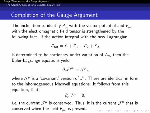
The inclination to identify Aµ with the vector potential and Fµνwith the electromagnetic field tensor is strengthened by thefollowing fact.
If the action integral with the new Lagrangian
Ltot = L+ L1 + L2 + L3
is determined to be stationary under variation of Aµ, then theEuler-Lagrange equations yield
∂νFµν = J µ,
where J µ is a ‘covariant’ version of Jµ. These are identical in formto the inhomogeneous Maxwell equations. It follows from thisequation, that
∂µJ µ = 0,
i.e. the current J µ is conserved. Thus, it is the current J µ that isconserved when the field Fµν is present.
Gauge Theories and the Gauge Argument
The Gauge Argument for a Complex Scalar Field
Completion of the Gauge Argument
The inclination to identify Aµ with the vector potential and Fµνwith the electromagnetic field tensor is strengthened by thefollowing fact. If the action integral with the new Lagrangian
Ltot = L+ L1 + L2 + L3
is determined to be stationary under variation of Aµ, then theEuler-Lagrange equations yield
∂νFµν = J µ,
where J µ is a ‘covariant’ version of Jµ. These are identical in formto the inhomogeneous Maxwell equations.
It follows from thisequation, that
∂µJ µ = 0,
i.e. the current J µ is conserved. Thus, it is the current J µ that isconserved when the field Fµν is present.
Gauge Theories and the Gauge Argument
The Gauge Argument for a Complex Scalar Field
Completion of the Gauge Argument
The inclination to identify Aµ with the vector potential and Fµνwith the electromagnetic field tensor is strengthened by thefollowing fact. If the action integral with the new Lagrangian
Ltot = L+ L1 + L2 + L3
is determined to be stationary under variation of Aµ, then theEuler-Lagrange equations yield
∂νFµν = J µ,
where J µ is a ‘covariant’ version of Jµ. These are identical in formto the inhomogeneous Maxwell equations. It follows from thisequation, that
∂µJ µ = 0,
i.e. the current J µ is conserved.
Thus, it is the current J µ that isconserved when the field Fµν is present.
Gauge Theories and the Gauge Argument
The Gauge Argument for a Complex Scalar Field
Completion of the Gauge Argument
The inclination to identify Aµ with the vector potential and Fµνwith the electromagnetic field tensor is strengthened by thefollowing fact. If the action integral with the new Lagrangian
Ltot = L+ L1 + L2 + L3
is determined to be stationary under variation of Aµ, then theEuler-Lagrange equations yield
∂νFµν = J µ,
where J µ is a ‘covariant’ version of Jµ. These are identical in formto the inhomogeneous Maxwell equations. It follows from thisequation, that
∂µJ µ = 0,
i.e. the current J µ is conserved. Thus, it is the current J µ that isconserved when the field Fµν is present.
Gauge Theories and the Gauge Argument
The Gauge Argument for a Complex Scalar Field
Completion of the Gauge Argument
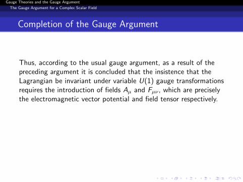
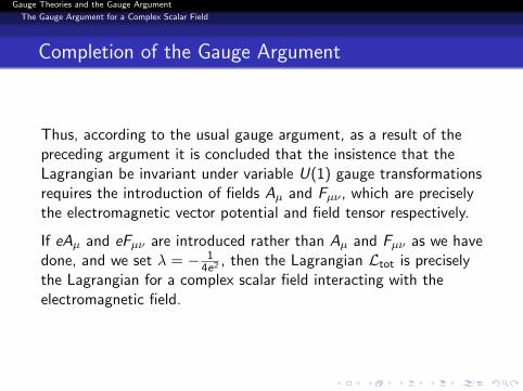
Thus, according to the usual gauge argument, as a result of thepreceding argument it is concluded that the insistence that theLagrangian be invariant under variable U(1) gauge transformationsrequires the introduction of fields Aµ and Fµν , which are preciselythe electromagnetic vector potential and field tensor respectively.
If eAµ and eFµν are introduced rather than Aµ and Fµν as we havedone, and we set λ = − 1
4e2 , then the Lagrangian Ltot is preciselythe Lagrangian for a complex scalar field interacting with theelectromagnetic field.
Gauge Theories and the Gauge Argument
The Gauge Argument for a Complex Scalar Field
Completion of the Gauge Argument
Thus, according to the usual gauge argument, as a result of thepreceding argument it is concluded that the insistence that theLagrangian be invariant under variable U(1) gauge transformationsrequires the introduction of fields Aµ and Fµν , which are preciselythe electromagnetic vector potential and field tensor respectively.
If eAµ and eFµν are introduced rather than Aµ and Fµν as we havedone, and we set λ = − 1
4e2 , then the Lagrangian Ltot is preciselythe Lagrangian for a complex scalar field interacting with theelectromagnetic field.
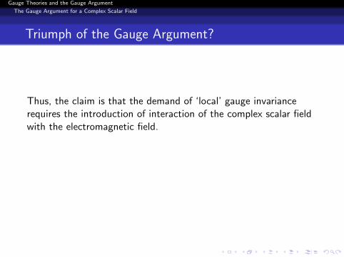
Gauge Theories and the Gauge Argument
The Gauge Argument for a Complex Scalar Field
Triumph of the Gauge Argument?
Thus, the claim is that the demand of ‘local’ gauge invariancerequires the introduction of interaction of the complex scalar fieldwith the electromagnetic field.
If the same pattern of reasoning is applied to a Dirac field, i.e.starting from the Dirac Lagrangian for a spin- 1
2 field, rather than aKlein-Gordon (spin-0) field, then Ltot ends up being theLagrangian density for quantum electrodynamics.
Gauge Theories and the Gauge Argument
The Gauge Argument for a Complex Scalar Field
Questioning the Gauge Argument
The last part of the gauge argument, i.e. the part that ‘naturally’leads to the introduction of the electromagnetic field, has aweakness.
The term L3 is not the only term that can be added to theLagrangian that depends only on Aµ and is gauge and Lorentzinvariant.
Gauge Theories and the Gauge Argument
The Gauge Argument for a Complex Scalar Field
Questioning the Gauge Argument
Healey points out, however, that it has been shown byO’Raifeartaigh (1979) that just introducing the term −1
4 FµνFµν
“yields the simplest, renormalizable, Lorentz- and “locally”gauge-invariant Lagrangian yielding the second-order equations ofmotion for the coupled system.” (166-167)
Healey adds that
So while the presence of this lacuna further underminesthe soundness of the gauge argument, it does little toweaken the associated explanation of the properties ofelectromagnetism. (167)
This argument does not work for QCD, however. . .
Gauge Theories and the Gauge Argument
The Gauge Argument for a Complex Scalar Field
Questioning the Gauge Argument
Healey points out, however, that it has been shown byO’Raifeartaigh (1979) that just introducing the term −1
4 FµνFµν
“yields the simplest, renormalizable, Lorentz- and “locally”gauge-invariant Lagrangian yielding the second-order equations ofmotion for the coupled system.” (166-167) Healey adds that
So while the presence of this lacuna further underminesthe soundness of the gauge argument, it does little toweaken the associated explanation of the properties ofelectromagnetism. (167)
This argument does not work for QCD, however. . .
Gauge Theories and the Gauge Argument
The Gauge Argument for a Complex Scalar Field
Status of the Gauge Argument
Healey’s overall comment on the gauge argument is the following:
. . . while the gauge argument effects a significantexplanatory unification among the properties of diversefundamental interactions, it certainly does not dictatetheir very existence. And while observations of chargeconservation may yield indirect support for an empiricalconstant phase symmetry of matter fields, the gaugeargument neither rests on nor entails a principle of“local” gauge symmetry with any empirical import, director indirect. “Local” gauge symmetry is a theoretical, notan empirical, symmetry. It is merely a feature of the waygauge theories of electromagnetic, electroweak, andstrong interactions are conventionally formulated. (167)
Gauge Theories and the Gauge Argument
Yang-Mills Theory
1 Gauge Theories
2 Classical Electromagnetism
3 Lagrangian Mechanics of FieldsLagrangian Mechanics of Point ParticlesLagrangian Mechanics of FieldsRelativistic Field Theories
4 The Gauge Argument for a Complex Scalar Field
5 Yang-Mills Theory
Gauge Theories and the Gauge Argument
Yang-Mills Theory
Extension of the Gauge Argument
Yang and Mills extended the gauge argument to examine fieldsthat are invariant under larger groups of internal transformations.
Yang and Mills considered a field with three real components thatis invariant under SU(2). This introduces new difficulties, since itis a non-abelian group.
Gauge Theories and the Gauge Argument
Yang-Mills Theory
Extension of the Gauge Argument
Yang and Mills extended the gauge argument to examine fieldsthat are invariant under larger groups of internal transformations.Yang and Mills considered a field with three real components thatis invariant under SU(2).
This introduces new difficulties, since itis a non-abelian group.
Gauge Theories and the Gauge Argument
Yang-Mills Theory
Extension of the Gauge Argument
Yang and Mills extended the gauge argument to examine fieldsthat are invariant under larger groups of internal transformations.Yang and Mills considered a field with three real components thatis invariant under SU(2). This introduces new difficulties, since itis a non-abelian group.
Gauge Theories and the Gauge Argument
Yang-Mills Theory
Yang-Mills Field
Using a gauge argument, the requirement that the Lagrangian beinvariant under ‘local’, i.e. variable, SU(2) transformations requiresthe introduction of a new field Wµ, which is the analogue of Aµ,but has three 4-vector components.
The analogue of Fµν is a 3-vector with second rank tensorcomponents Wµν , which is obtained from Wµ according to anequation like that of Fµν in terms of Aµ in the U(1) case but withan additional term
gWµ ×Wν .
It is that the symmetry group is non-abelian that leads to theintroduction of this term. This term has interesting implications,which includes the fact that the gauge field Wµν is self-interacting,i.e. it is a source for itself.
Gauge Theories and the Gauge Argument
Yang-Mills Theory
Yang-Mills Field
Using a gauge argument, the requirement that the Lagrangian beinvariant under ‘local’, i.e. variable, SU(2) transformations requiresthe introduction of a new field Wµ, which is the analogue of Aµ,but has three 4-vector components.
The analogue of Fµν is a 3-vector with second rank tensorcomponents Wµν
, which is obtained from Wµ according to anequation like that of Fµν in terms of Aµ in the U(1) case but withan additional term
gWµ ×Wν .
It is that the symmetry group is non-abelian that leads to theintroduction of this term. This term has interesting implications,which includes the fact that the gauge field Wµν is self-interacting,i.e. it is a source for itself.
Gauge Theories and the Gauge Argument
Yang-Mills Theory
Yang-Mills Field
Using a gauge argument, the requirement that the Lagrangian beinvariant under ‘local’, i.e. variable, SU(2) transformations requiresthe introduction of a new field Wµ, which is the analogue of Aµ,but has three 4-vector components.
The analogue of Fµν is a 3-vector with second rank tensorcomponents Wµν , which is obtained from Wµ according to anequation like that of Fµν in terms of Aµ in the U(1) case but withan additional term
gWµ ×Wν .
It is that the symmetry group is non-abelian that leads to theintroduction of this term. This term has interesting implications,which includes the fact that the gauge field Wµν is self-interacting,i.e. it is a source for itself.
Gauge Theories and the Gauge Argument
Yang-Mills Theory
Yang-Mills Field
Using a gauge argument, the requirement that the Lagrangian beinvariant under ‘local’, i.e. variable, SU(2) transformations requiresthe introduction of a new field Wµ, which is the analogue of Aµ,but has three 4-vector components.
The analogue of Fµν is a 3-vector with second rank tensorcomponents Wµν , which is obtained from Wµ according to anequation like that of Fµν in terms of Aµ in the U(1) case but withan additional term
gWµ ×Wν .
It is that the symmetry group is non-abelian that leads to theintroduction of this term. This term has interesting implications,which includes the fact that the gauge field Wµν is self-interacting,i.e. it is a source for itself.
Gauge Theories and the Gauge Argument
Yang-Mills Theory
Too Bad for Yang and Mills, However. . .
It turns out that the theory developed by Yang and Mills is notinstantiated in nature. Their method of how to develop the gaugeargument for a non-abelian symmetry group G has beengeneralized and has found application, however.
For G = SU(3), the classical field theory that is quantized toyield quantum chromodynamics can be obtained;
For G = U(1)⊗ SU(2), the classical field theory used todevelop electroweak theory can be obtained.
In case that G = U(1) the classical field theory that whenquantized yields quantum electrodynamics can obtained, whichbecomes a particular case of the general Yang-Mills argument. Forthis reason the quantum field theories of the standard model canall be considered Yang-Mills theories.
Gauge Theories and the Gauge Argument
Yang-Mills Theory
Too Bad for Yang and Mills, However. . .
It turns out that the theory developed by Yang and Mills is notinstantiated in nature. Their method of how to develop the gaugeargument for a non-abelian symmetry group G has beengeneralized and has found application, however.
For G = SU(3), the classical field theory that is quantized toyield quantum chromodynamics can be obtained;
For G = U(1)⊗ SU(2), the classical field theory used todevelop electroweak theory can be obtained.
In case that G = U(1) the classical field theory that whenquantized yields quantum electrodynamics can obtained, whichbecomes a particular case of the general Yang-Mills argument.
Forthis reason the quantum field theories of the standard model canall be considered Yang-Mills theories.
Gauge Theories and the Gauge Argument
Yang-Mills Theory
Too Bad for Yang and Mills, However. . .
It turns out that the theory developed by Yang and Mills is notinstantiated in nature. Their method of how to develop the gaugeargument for a non-abelian symmetry group G has beengeneralized and has found application, however.
For G = SU(3), the classical field theory that is quantized toyield quantum chromodynamics can be obtained;
For G = U(1)⊗ SU(2), the classical field theory used todevelop electroweak theory can be obtained.
In case that G = U(1) the classical field theory that whenquantized yields quantum electrodynamics can obtained, whichbecomes a particular case of the general Yang-Mills argument. Forthis reason the quantum field theories of the standard model canall be considered Yang-Mills theories.
Gauge Theories and the Gauge Argument
References
Baez, John and Javier P. Muniain. Gauge Fields, Knots andGravity. New Jersey: World Scientific, 1994.
Goldstein, Herbert, Charles Poole and John Safko. ClassicalMechanics. 3rd Ed. Toronto: Addison Wesley, 2002.
Griffiths, David. Introduction to Elementary Particles. NewYork: John Wiley & Sons, 1987.
Healey, Richard. Gauging What’s Real: The ConceptualFoundations of Contemporary Gauge Theories. New York:Oxford University Press, 2007.
Jackson, John David. Classical Electrodynamics. New York:John Wiley & Sons, 1999.
Ryder, Lewis H. Quantum Field Theory. 2nd Ed. Cambridge:Cambridge University Press, 1996.