guidelines for harvesting species of different lifespans · mrag guidelines for harvesting species...
TRANSCRIPT
Guidelines for HarvestingSpecies of Different Lifespans
Project R. 4823
Draft Final Report for the Overseas Development Administration
Fisheries Management Science Programme
MRAG Ltd June 1994

DRAFT FINAL REPORT
Reporting period: 1 January 1992 - 30 June 1994
Name: Dr G. P. Kirkwood
Signature:
MRAG Ltd27 Campden StreetLondon W8 7EPUK
MRAG GUIDELINES FOR HARVESTING SPECIES OF DIFFERENT LIFESPANS S FINAL REPORT MRAG
CONTENTS
FINAL REPORT . . . . . . . . . . . . . . . . . . . . . . . . . . . . . . . . . . . . . . . . . . . . . . . . . . . . . . . . . . . . . . . . . 1
1. Objective of the project . . . . . . . . . . . . . . . . . . . . . . . . . . . . . . . . . . . . . . . . . . . . . . . 1
2. Work carried out . . . . . . . . . . . . . . . . . . . . . . . . . . . . . . . . . . . . . . . . . . . . . . . . . . . . 1
3. Results . . . . . . . . . . . . . . . . . . . . . . . . . . . . . . . . . . . . . . . . . . . . . . . . . . . . . . . . . . . 2
4. Implications of the results for achieving the objectives . . . . . . . . . . . . . . . . . . . . . . 7
5. Priority tasks for follow up . . . . . . . . . . . . . . . . . . . . . . . . . . . . . . . . . . . . . . . . . . . . 7
OUTLINE OF RESULTS OBTAINED . . . . . . . . . . . . . . . . . . . . . . . . . . . . . . . . . . . . . . . . . . . . . . . . . 9
1. Introduction . . . . . . . . . . . . . . . . . . . . . . . . . . . . . . . . . . . . . . . . . . . . . . . . . . . . . . . . 9
2. Methods . . . . . . . . . . . . . . . . . . . . . . . . . . . . . . . . . . . . . . . . . . . . . . . . . . . . . . . . . . 10
2.1 Population dynamics model . . . . . . . . . . . . . . . . . . . . . . . . . . . . . . . . . . . . 10
2.2 Typical values of parameters . . . . . . . . . . . . . . . . . . . . . . . . . . . . . . . . . . . . 18
3. Sustainable yields for constant recruitment . . . . . . . . . . . . . . . . . . . . . . . . . . . . . . . 22
4. Allowing for a stock-recruitment relationship . . . . . . . . . . . . . . . . . . . . . . . . . . . . . . 24
4.1 Nature of relationship between yield-biomass ratio and M . . . . . . . . . . . . . 24
4.2 Nature of relationship between FMSY and M . . . . . . . . . . . . . . . . . . . . . . . . . 30
4.3 Approximate constants of proportionality between yield-biomass
ratios and M and between FMSY and M . . . . . . . . . . . . . . . . . . . . . . . . . . . . 35
4.4 An empirical formula . . . . . . . . . . . . . . . . . . . . . . . . . . . . . . . . . . . . . . . . . . 45
5. Effect of age-dependent natural mortality . . . . . . . . . . . . . . . . . . . . . . . . . . . . . . . . . 45
6. The special case of very short-lived species . . . . . . . . . . . . . . . . . . . . . . . . . . . . . . 46
7. Estimates of yield-biomass ratios and FMSY for selected species . . . . . . . . . . . . . . . 48
8. Stochastic recruitment . . . . . . . . . . . . . . . . . . . . . . . . . . . . . . . . . . . . . . . . . . . . . . . 54
8.1 Environmental variability in recruitment . . . . . . . . . . . . . . . . . . . . . . . . . . . . 54
8.2 Recovery from a stock collapse . . . . . . . . . . . . . . . . . . . . . . . . . . . . . . . . . 55
9. Conclusions . . . . . . . . . . . . . . . . . . . . . . . . . . . . . . . . . . . . . . . . . . . . . . . . . . . . . . . 56
10. References . . . . . . . . . . . . . . . . . . . . . . . . . . . . . . . . . . . . . . . . . . . . . . . . . . . . . . . . 57
1 Kirkwood, G.P., Beddington, J.R. and J.A. Rossouw. 1994. Harvesting species of different lifespans. pp199-227 in Edwards,P.J., May, R. and Webb, N.R. (Eds) "Large Scale Ecology and Conservation Biology". Blackwell Scientific Publications.
Beddington, J.R. and M. Basson. 1994. The limits to exploitation on land and sea. Phil. Trans. Roy. Soc. Lond. B. 343: 87-92
MRAG GUIDELINES FOR HARVESTING SPECIES OF DIFFERENT LIFESPANS S FINAL REPORT 1
FINAL REPORT
R. 4823 Guidelines for harvesting species of different life spans
1. Objective of the project
The objective of this project was to develop simple guidelines, underpinned by rigorous mathematicalanalysis, for the harvesting of fish species with different lifespans.
2. Work carried out
A computer program implementing an extremely flexible, fully age-structured simulation model of thedynamics of exploited fish stocks has been developed. The mathematical structure of the model of thedynamics of exploited fish populations is similar to that described by Beverton and Holt. The key biologicalparameters are the rate of natural mortality (M), the growth rate of the species (K) and the size at whichsexual maturity is reached. The primary variables that can be manipulated to adjust yield levels are thesize at which exploitation begins and the fishing mortality rate imposed by harvesting.
Population regulation via density dependence is allowed for in the model through incorporation of a non-linear relationship between the spawning stock biomass and the subsequent recruitment of juvenile fishto the population. Of the several frequently used stock-recruitment relationships in fisheries models, mostattention has been given here to the Beverton and Holt version, which has the twin advantages of havinga simple mathematical form, and of being relatively conservative in the degree of density dependence itattributes to the population. Results have also been obtained, however, for the Ricker form of the stock-recruitment relationship, which allows for higher degrees of density dependent regulation. Stochasticvariability in recruitment is also allowed in the model.
The computer program was used to examine the way the maximum sustainable yield of a fish stock,measured as a proportion of its unexploited biomass, varied as a function of the key biological parameters,and of the size at which exploitation first commences (the size at first capture). In particular, simpleguidelines for harvesting were sought by examining the relationship between yield-biomass ratios and thenatural mortality rate, and the relationship between the fishing mortality rate producing maximum yield andthe natural mortality rate. The results obtained have been documented in two scientific papers1, one whichwas presented to the British Ecological Society Symposium on Large Scale Ecology and ConservationBiology, and the other to the Royal Society discussion meeting on Generalizing Across Marine andTerrestrial Ecology. Reprints of the papers are appended to this report.
MRAG has entered into a formal agreement with the International Center for Living Aquatic ResourcesManagement (ICLARM) to be a collaborator in the FISHBASE project, which they are conducting jointlywith FAO. As part of that agreement, access has been obtained to a development version of a veryextensive database of estimates of biological parameters for a wide range of fish species. Access has alsobeen obtained to a comprehensive set of stock-recruitment data for over 100 fish stocks. These two datasources have been used to develop tables of estimates of yield-biomass ratios and fishing mortality ratesfor key fish species.
2 GUIDELINES FOR HARVESTING SPECIES OF DIFFERENT LIFESPANS S FINAL REPORT MRAG
3. Results
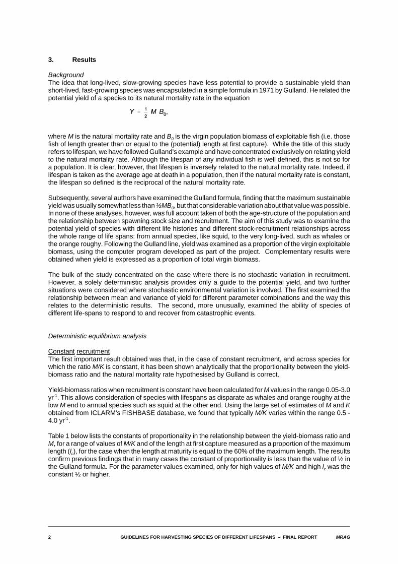
BackgroundThe idea that long-lived, slow-growing species have less potential to provide a sustainable yield thanshort-lived, fast-growing species was encapsulated in a simple formula in 1971 by Gulland. He related thepotential yield of a species to its natural mortality rate in the equation
where M is the natural mortality rate and B0 is the virgin population biomass of exploitable fish (i.e. thosefish of length greater than or equal to the (potential) length at first capture). While the title of this studyrefers to lifespan, we have followed Gulland's example and have concentrated exclusively on relating yieldto the natural mortality rate. Although the lifespan of any individual fish is well defined, this is not so fora population. It is clear, however, that lifespan is inversely related to the natural mortality rate. Indeed, iflifespan is taken as the average age at death in a population, then if the natural mortality rate is constant,the lifespan so defined is the reciprocal of the natural mortality rate.
Subsequently, several authors have examined the Gulland formula, finding that the maximum sustainableyield was usually somewhat less than ½MB0, but that considerable variation about that value was possible.In none of these analyses, however, was full account taken of both the age-structure of the population andthe relationship between spawning stock size and recruitment. The aim of this study was to examine thepotential yield of species with different life histories and different stock-recruitment relationships acrossthe whole range of life spans: from annual species, like squid, to the very long-lived, such as whales orthe orange roughy. Following the Gulland line, yield was examined as a proportion of the virgin exploitablebiomass, using the computer program developed as part of the project. Complementary results wereobtained when yield is expressed as a proportion of total virgin biomass.
The bulk of the study concentrated on the case where there is no stochastic variation in recruitment.However, a solely deterministic analysis provides only a guide to the potential yield, and two furthersituations were considered where stochastic environmental variation is involved. The first examined therelationship between mean and variance of yield for different parameter combinations and the way thisrelates to the deterministic results. The second, more unusually, examined the ability of species ofdifferent life-spans to respond to and recover from catastrophic events.
Deterministic equilibrium analysis
Constant recruitmentThe first important result obtained was that, in the case of constant recruitment, and across species forwhich the ratio M/K is constant, it has been shown analytically that the proportionality between the yield-biomass ratio and the natural mortality rate hypothesised by Gulland is correct.
Yield-biomass ratios when recruitment is constant have been calculated for M values in the range 0.05-3.0yr-1. This allows consideration of species with lifespans as disparate as whales and orange roughy at thelow M end to annual species such as squid at the other end. Using the large set of estimates of M and Kobtained from ICLARM's FISHBASE database, we found that typically M/K varies within the range 0.5 -4.0 yr-1.
Table 1 below lists the constants of proportionality in the relationship between the yield-biomass ratio andM, for a range of values of M/K and of the length at first capture measured as a proportion of the maximumlength (lc), for the case when the length at maturity is equal to the 60% of the maximum length. The resultsconfirm previous findings that in many cases the constant of proportionality is less than the value of ½ inthe Gulland formula. For the parameter values examined, only for high values of M/K and high lc was theconstant ½ or higher.

MRAG GUIDELINES FOR HARVESTING SPECIES OF DIFFERENT LIFESPANS S FINAL REPORT 3
Table 1. Constants of proportionality in the relationship between the yield-biomass ratio and Mwhen recruitment is constant, for different values of lc and M/K.
M/K
lc 0.5 1.0 2.0 3.0 4.0
0.2 0.30 0.25 0.22 0.22 0.22
0.4 0.35 0.32 0.32 0.36 0.41
0.6 0.45 0.44 0.52 0.60 0.66
0.8 0.63 0.69 0.77 0.82 0.85
The corresponding fishing mortality rates measured as a proportion of M are given in Table 2.
Table 2. Fishing mortality rates producing maximum yield as a proportion of M when recruitmentis constant, for different values of lc and M/K.
M/K
lc 0.5 1.0 2.0 3.0 4.0
0.2 1.10 0.89 0.81 0.85 0.94
0.4 1.45 1.37 1.79 3.01 9.60
0.6 2.40 3.20 4 4 4
0.8 10.20 4 4 4 4
Table 1 illustrates that the proportion of the exploitable biomass that can be taken sustainably increasesconsiderably with length at first capture. It should be noted, however, that while the proportion ofexploitable biomass that can be taken increases with lc, the exploitable biomass itself decreases. Whenmeasured as a ratio of yield to total biomass, the corresponding constant of proportionality actuallydecreases. When M/K varies even over the wide range of 0.5-4.0, Table 1 shows that the constants ofproportionality are rather similar for a given lc.
Alternative stock-recruitment relationshipsGiven the direct proportionality found between the yield-biomass ratio and M when recruitment is constant,it was tempting to hypothesise that the same relationship might hold when recruitment varies as a functionof the size of the spawning stock. Unfortunately, this turned out not to be true, but for many biologicallylikely parameter combinations the relationship was found to be very close to proportional for all practicalpurposes.
For the Beverton-Holt stock-recruitment relationship, the higher the degree of density dependence(measured as a parameter d taking values in the range 0 to 1; see appended papers), the less doesrecruitment decline as the spawning stock size is reduced below unexploited levels. In the limit withmaximal density dependence, recruitment is constant regardless of spawning stock size. Results obtainedindicate that the approximate constant of proportionality in the relation between yield-biomass ratio andM increases as the degree of density dependence increases.
This finding, of course, implies that for fish stocks that exhibit low degrees of density dependence, theGulland formula is even more optimistic that was suggested above. Table 1 indicates that yield taken asa percentage of virgin exploitable biomass is more likely to be around 0.3M than the 0.5M that Gullandsuggested. When more realistic levels of density dependence are considered, the percentage yield isfurther reduced, perhaps to between 0.1M and 0.2M.
4 GUIDELINES FOR HARVESTING SPECIES OF DIFFERENT LIFESPANS S FINAL REPORT MRAG
Inspection of the full set of empirical relationships obtained indicates that substantial departures fromproportionality between yield-biomass ratios and M occur only for quite high values of M (e.g. M>1) andprimarily when the degree of density dependence is also small. This particular combination of parametersis biologically the most unlikely: normally one expects that low degrees of density dependence in a stock-recruitment relation will be associated with species that have long life-spans and therefore low mortalityrates, and conversely that species with nearly constant recruitment even for small spawning stockbiomasses will be short-lived and fast growing.
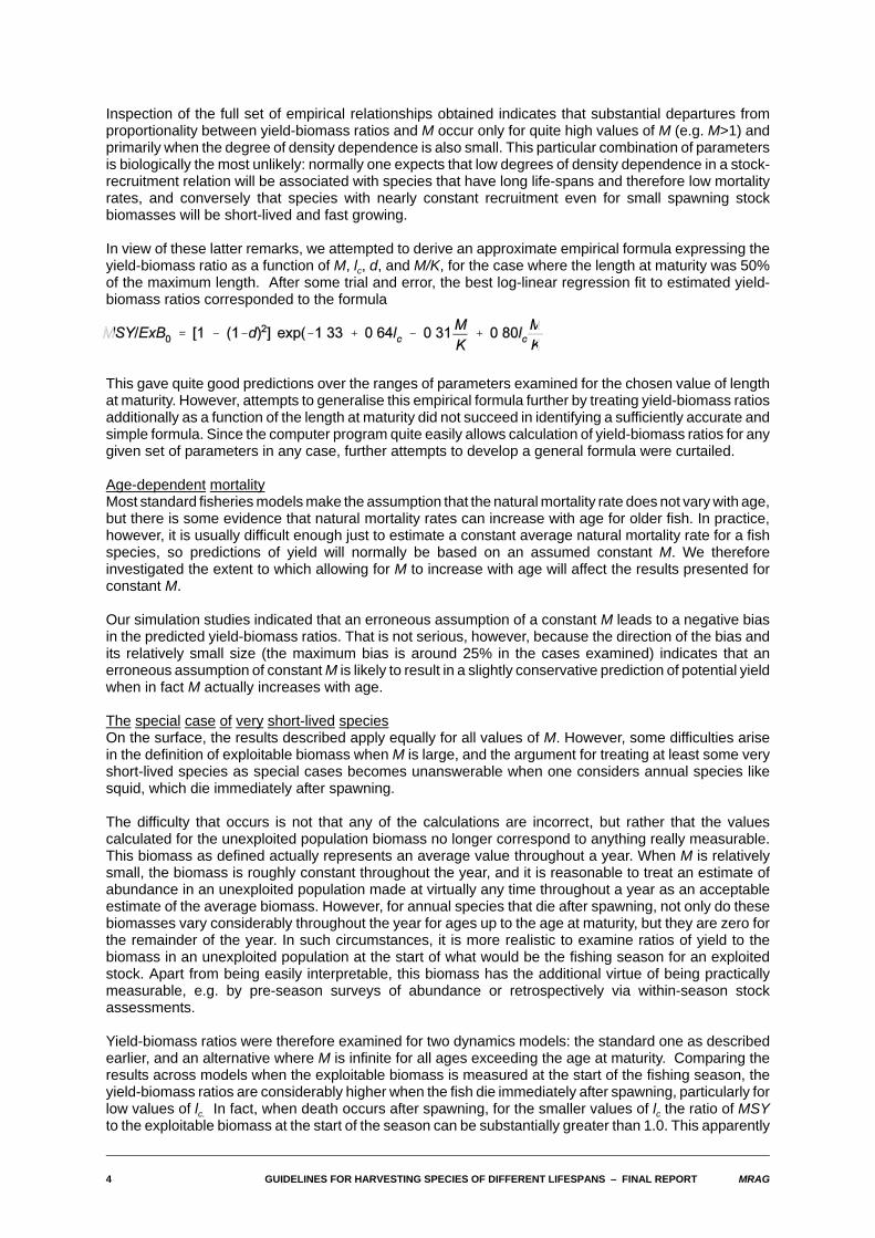
In view of these latter remarks, we attempted to derive an approximate empirical formula expressing theyield-biomass ratio as a function of M, lc, d, and M/K, for the case where the length at maturity was 50%of the maximum length. After some trial and error, the best log-linear regression fit to estimated yield-biomass ratios corresponded to the formula
This gave quite good predictions over the ranges of parameters examined for the chosen value of lengthat maturity. However, attempts to generalise this empirical formula further by treating yield-biomass ratiosadditionally as a function of the length at maturity did not succeed in identifying a sufficiently accurate andsimple formula. Since the computer program quite easily allows calculation of yield-biomass ratios for anygiven set of parameters in any case, further attempts to develop a general formula were curtailed.
Age-dependent mortalityMost standard fisheries models make the assumption that the natural mortality rate does not vary with age,but there is some evidence that natural mortality rates can increase with age for older fish. In practice,however, it is usually difficult enough just to estimate a constant average natural mortality rate for a fishspecies, so predictions of yield will normally be based on an assumed constant M. We thereforeinvestigated the extent to which allowing for M to increase with age will affect the results presented forconstant M.
Our simulation studies indicated that an erroneous assumption of a constant M leads to a negative biasin the predicted yield-biomass ratios. That is not serious, however, because the direction of the bias andits relatively small size (the maximum bias is around 25% in the cases examined) indicates that anerroneous assumption of constant M is likely to result in a slightly conservative prediction of potential yieldwhen in fact M actually increases with age.
The special case of very short-lived speciesOn the surface, the results described apply equally for all values of M. However, some difficulties arisein the definition of exploitable biomass when M is large, and the argument for treating at least some veryshort-lived species as special cases becomes unanswerable when one considers annual species likesquid, which die immediately after spawning.
The difficulty that occurs is not that any of the calculations are incorrect, but rather that the valuescalculated for the unexploited population biomass no longer correspond to anything really measurable.This biomass as defined actually represents an average value throughout a year. When M is relativelysmall, the biomass is roughly constant throughout the year, and it is reasonable to treat an estimate ofabundance in an unexploited population made at virtually any time throughout a year as an acceptableestimate of the average biomass. However, for annual species that die after spawning, not only do thesebiomasses vary considerably throughout the year for ages up to the age at maturity, but they are zero forthe remainder of the year. In such circumstances, it is more realistic to examine ratios of yield to thebiomass in an unexploited population at the start of what would be the fishing season for an exploitedstock. Apart from being easily interpretable, this biomass has the additional virtue of being practicallymeasurable, e.g. by pre-season surveys of abundance or retrospectively via within-season stockassessments.
Yield-biomass ratios were therefore examined for two dynamics models: the standard one as describedearlier, and an alternative where M is infinite for all ages exceeding the age at maturity. Comparing theresults across models when the exploitable biomass is measured at the start of the fishing season, theyield-biomass ratios are considerably higher when the fish die immediately after spawning, particularly forlow values of lc. In fact, when death occurs after spawning, for the smaller values of lc the ratio of MSYto the exploitable biomass at the start of the season can be substantially greater than 1.0. This apparently
MRAG GUIDELINES FOR HARVESTING SPECIES OF DIFFERENT LIFESPANS S FINAL REPORT 5
odd finding simply reflects the fact that fishing has started well before the population has reached itsmaximum biomass for the year.
Estimates of yield-biomass ratios and fishing mortality rates for selected speciesUsing estimates of biological and fishery-related parameters contained in the FISHBASE database, aswell as estimates of stock-recruitment parameters obtained from other sources, preliminary estimates ofyield-biomass ratios and fishing mortality rates have been obtained for 53 commercially exploited orexploitable marine fish species. Tables of these are included in the summary report appended. Clearly asthe amount of information recorded on the database increases, this table can be extended.
The effect of stochastic recruitmentIn their examination of the statistical properties of recruitment in some commercial fish species, severalauthors have found that the frequency distribution of annual recruitment was similar to that of a log-normaldistribution. Accordingly, we investigated the probability distribution of annual yield when the annualrecruitment is log-normally distributed with mean equal to that predicted by the deterministic Beverton-Holtstock-recruitment relationship.
For low values of M, the median annual yield-biomass ratio was found to be very close to thecorresponding deterministic value, but as M increased, the median began to fall below the deterministicvalue. There was a strong tendency for increased skewness in the distribution of annual yield-biomassratios as M increases.
A direct result of the increasing skewness with M is that, while in most cases the annual yield-biomassratio will be much less than ½M, in an important minority of cases it can exceed ½M, sometimessubstantially. This ability to gain benefits in terms of high yields during good years flows directly from theassumption that fishing mortality (or equivalently fishing effort) is the variable that is used to control thelevel of harvesting. If harvesting is controlled by pre-set annual catch quotas, this benefit will not beavailable, and unless the quotas are set conservatively there can be an important risk of stock collapse.
Recovery from a stock collapseWe also examined the ability of a population to recover from a catastrophic mortality episode. Specifically,we examined a case in which a population is initially in equilibrium, being harvested at the fishing mortalityrate that produces the deterministic MSY. Just before the start of the spawning season in the first year,it is assumed that the entire spawning stock dies, so that there is no recruitment at all at the beginning ofthe second year. Subsequently, the population is allowed to recover, if it can. During the recovery period,fishing continues at the same rate.
For each case where M was sufficiently low that the age at maturity is greater than one year, the spawningstock biomasses recovered (eventually) despite continued exploitation. The key to the recovery was thatthe unfished age-classes in longer-lived species provided a buffer against such catastrophic events. Incontrast, under the conditions simulated any species with M sufficiently high that the age at maturity is lessthan one year will by definition be completely extinguished by the catastrophe hypothesised. This mayseem an extremely unlikely scenario, but all that is required to bring about conditions nearly matchingthose simulated is for the species to have a critical spawning biomass below which recruitment is severelydiminished. Then a bout of overfishing, for example, could well result in an almost complete stockcollapse.
It follows that in this sense, longer-lived species can show a greater resilience than short-lived ones.Further, the greater the number of unfished age-classes, the greater the amount of buffering. Thusextremely long-lived fish species, such as orange roughy, have the ability to withstand occasional majorcatastrophic events, despite the very low sustainable yields they provide.
Summary conclusions
The primary conclusion that may be drawn is that although there is a clear approximately proportionalrelationship between sustainable yield and natural mortality, the constant of proportionality is smaller thanhad originally been proposed by Gulland. Even in the case where recruitment remains constant regardlessof how small the mature stock size is, yield taken as a percentage of virgin exploitable biomass is morelikely to be around 0.3M, rather than the 0.5M that Gulland suggested. When more realistic levels ofdensity dependence are considered, the percentage yield is further reduced, perhaps to between 0.1M
6 GUIDELINES FOR HARVESTING SPECIES OF DIFFERENT LIFESPANS S FINAL REPORT MRAG
and 0.2M.
When looked at specifically in terms of lifespans, the non-linear relationship between M and lifespanimplies that for longer-lived species, the sustainable yields are both low and almost independent oflifespan. An exception to this ground rule is the behaviour of very short lived species. In these species,the details of the life cycle dominate their response to exploitation, such that on sensible and measurabledefinitions of exploitable biomass, the stock may be capable of producing sustainable yields well in excessof the biomass measured at the start of the fishing season.
Tables of yield-biomass ratios and fishing mortality rates have been calculated for a wide range of valuesof the key biological and fishery-related parameters. These are included in the attached outline of results.These tables will allow estimation (by interpolation if necessary) of yield-biomass ratios and fishingmortality rates for most species, given values of the appropriate parameters. In addition, however, a tableof estimates of yield-biomass ratios and fishing mortality rates for 53 selected commercially exploitedmarine fish species has also been calculated, using information contained in the FISHBASE database andother sources. This has been included in the attached outline of results.
The deterministic results are a useful guide to expectations in the real world, particularly for relatively long-lived species. The investigation of stochasticity in recruitment and its implications for the expectedvariation in yield complements other findings that a management policy of constant effort with a target levelof fishing mortality can produce substantial benefits in terms of high yields when recruitment is high. Thestrength of this effect with increasing mortality (reduced lifespan) is particularly marked.
While very short-lived species can provide high yields, the brief examination of the effect of catastrophicevents on their dynamics indicates that longer-lived species retain a resilience to catastrophes that is notavailable to the short-lived species, which can be particularly vulnerable to a combination of highexploitation and occasional environmental events that devastate the spawning stock.
A more detailed description of results obtained immediately follows this final project report. Publishedscientific papers arising from this research are also appended.
MRAG GUIDELINES FOR HARVESTING SPECIES OF DIFFERENT LIFESPANS S FINAL REPORT 7
4. Implications of the results for achieving the objectives
As the results outlined above indicate, this project has been very successful in achieving its objectives.Analysis of a detailed rigorous mathematical model for the dynamics of fish stocks, incorporating both age-structure and density dependence in the form of a stock-recruitment relationship, has revealed simple andpractical guidelines for calculating the maximum sustainable yield available from a stock in terms of thevirgin exploitable biomass and the natural mortality rate. Similar guidelines are also available for thefishing mortality rate producing maximum yield as a proportion of the natural mortality rate. The computerprogram developed for this project also allows explicit calculation of yield-biomass ratios given estimatesof key biological and technical parameters. This has been used in conjunction with fisheries databasessuch as FISHBASE and comparable compilations of estimated stock-recruitment relationships to obtainestimates of yield-biomass ratios for a number of important fish stocks.
5. Priority tasks for follow up
The results obtained in this project set the scene for more detailed investigations of individual species andgroups of species, both in terms of extending the range of species for which individual estimates of yield-biomass ratios and fishing mortality rates have been calculated, and in terms of examining the way inwhich the key parameters that determine yields vary. In this latter context, the dependence found by Paulybetween natural mortality, growth in size, and mean water temperature for a wide range of fish stocksaffords the possibility of further assessment of the potential yields of species in marine ecosystems ofdifferent types.
The final report details estimates of yield-biomass ratios for important fish species for which the currentversion of the FISHBASE database contains estimates of the key parameters. This database is still underdevelopment by ICLARM and FAO and it is anticipated that over time the range of species for which keyparameter estimates are available will expand greatly. Also, the computer software packages LFDA andCEDA developed by MRAG under another Fisheries Management Science project allow independentestimation of several of the key biological parameters used in the calculation of yield-biomass ratio. Ittherefore seems desirable that any subsequent adaptive phase for this project should include developmentof appropriate computer software with accompanying manuals for the direct calculation of yield-biomassratios.

8 GUIDELINES FOR HARVESTING SPECIES OF DIFFERENT LIFESPANS S FINAL REPORT MRAG
MRAG GUIDELINES FOR HARVESTING SPECIES OF DIFFERENT LIFESPANS S FINAL REPORT 9
OUTLINE OF RESULTS OBTAINED
1. Introduction
The idea that long-lived, slow-growing species have less potential to provide a sustainable yield thanshort-lived, fast-growing species was first encapsulated in a simple formula by Gulland (1971). Thisformula directly related the potential yield of a species to its natural mortality rate in the equation
where M is the natural mortality rate and B0 is the virgin exploitable population biomass.
Gulland's argument was a simple mix of a theoretical consideration, that the level at which maximumsustainable yield can be obtained occurs at ½ the unexploited level in a simple logistic model, and anobservation from experience of fisheries world-wide that indicated that the maximum yield appeared tooccur when the level of fishing mortality was roughly equal to that of natural mortality.
While the title of this study refers to lifespan, we have followed Gulland's example and have concentratedexclusively on relating yield to the natural mortality rate. While the lifespan of any individual fish is welldefined, this is not so for a population. It is clear, however, that lifespan is inversely related to M. Indeed,if lifespan is taken as the average age at death in a population, then if M is constant, the lifespan sodefined is the reciprocal of M.
In the context of generalised stock production models, of which the logistic model is one simple example,the Gulland formula was re-examined by Shepherd (1982). He found that the maximum sustainable yieldwas usually somewhat less than ½MB0, but variation by a factor of three either way about that value waspossible. However, Shepherd's analysis did not take age-structure into account.
Beddington and Cooke (1983) examined the Gulland formula using a more detailed age-structured model.In their analysis, they distinguished between the yield as a proportion of the exploitable biomass (definedas the biomass above the age or length at which exploitation starts) and the total biomass. Clearly, thisdistinction is particularly significant in cases where exploitation starts at a relatively advanced age.Results were presented for a range of life-spans of typical commercially exploited fish. They found theGulland formula tended to be optimistic, with the potential yield being somewhat lower than it predicted.Their analysis was further restricted by a decision to examine recruitment in a simple way. It was assumedconstant above a threshold adult biomass.
The aim of this project was to examine in a general way the potential yield of species with different lifehistories and different stock-recruitment relationships across the whole range of life spans: from annualspecies, like squid, to the very long-lived, such as whales or the orange roughy.
Following the Gulland line, yield was examined as a proportion of the unexploited biomass. There arereally two interrelated levels of yield viewed in this way: that as a proportion of the total biomass and thatas a proportion of the exploitable biomass. The former is perhaps the more ecologically interesting, in thatit sets a limit to the yield that particular species in an ecosystem can provide. The latter lies more in thedomain of the fishery manager, who is interested in the limits of commercial exploitation, and has theability to adjust the age or length at which exploitation commences. Because this latter context is morenatural for the intended users of the guidelines developed, most attention was placed on determiningpotential yield as a proportion of virgin exploitable biomass
In our examination of the deterministic case, which takes up the bulk of this report, we demonstrate thatthe potential yield measured as a proportion of the virgin biomass is indeed approximately proportionalto the natural mortality rate, at least for biologically feasible combinations of parameters. The constants
10 GUIDELINES FOR HARVESTING SPECIES OF DIFFERENT LIFESPANS S FINAL REPORT MRAG
of proportionality are functions of the key parameters of growth, mortality (life span) and the densitydependent response as focused in the variation in recruitment with mature stock size. We also brieflyexamine the extent to which the presence of age-dependence in natural mortality might affect thepredictions.
Clearly, a solely deterministic analysis provides only a guide to the potential yield. Two situations wereexamined where environmental variation is involved. The first follows Beddington and May (1977) byexamining the relationship between mean and variance of yield for different parameter combinations andthe way this relates to the deterministic results. The second, more unusually, examines the ability ofspecies of different life-spans to respond to and recover from catastrophic events.
2. Methods
In this section, we first briefly outline the essentials of the models used to describe the populationdynamics of an exploited fish population. Readers interested in the detailed mathematical formulation arereferred to Kirkwood et al (1994), a copy of which is appended. Here, we will simply attempt to highlightthe main elements in the models and the role played by the key biological and fishery parameters. Wethen draw on information contained in the FISHBASE database being developed jointly by ICLARM andFAO to identify likely ranges of values for these key parameters.
2.1 Population dynamics model
Dynamics of a single cohortThe dynamics of the fish population are assumed to be described by an age-structured model incontinuous time. The model is formulated as a set of equations that, by and large, follow the mathematicalstructure of the dynamics of exploited fish populations described in Beverton and Holt (1957) and usedby Beddington and Cooke (1983). The key biological parameters are the rate of natural mortality, thegrowth rate of the species and the size at which sexual maturity is reached. The primary variables that canbe manipulated to adjust yield levels are the size at which exploitation begins and the mortality rateimposed by harvesting.
Consider first with the dynamics of a single cohort of fish, which initially consists of R fish born at age zero.
Let tc = the age at first exploitation of fish in the cohort;Lc = the length at first exploitation;tm = the age at sexual maturity;Lm = the length at sexual maturity;M = the instantaneous rate of natural mortality ;F = the instantaneous rate of fishing mortality;N(t) = the number of fish of age t years; andw(t) = the weight of fish of age t years;
The dynamics of the cohort are described by the following equations:
These equations assume that R fish recruit to the cohort at age zero. As they grow, their numbers diminishthrough the action of a constant exponential rate of natural mortality M until age tc. From age tc onwards,fishing also occurs at a constant exponential rate F. This latter assumption is equivalent to assuming thatthe selectivity of the fishing gear is constant on all fish aged tc and older. Adjustments would have to bemade if a highly selective gear is being used, or if fish migrate from the fishing grounds at a later stageof their life.
In an unfished cohort (F=0), the total biomass over its lifespan is
MRAG GUIDELINES FOR HARVESTING SPECIES OF DIFFERENT LIFESPANS S FINAL REPORT 11
This expression can be thought of as the sum over all ages of the surviving numbers at age t times theweight at age t. The exploitable biomass is given by an equivalent expression, except that now the "sum"is taken only over all ages greater than or equal to the age at first capture:
In common with standard fisheries practice, we assume that growth can be modelled by the vonBertalanffy (1938) growth curve, with the weight w(t) at age t given by
where W4 is the asymptotic weight, K is the growth rate and t0 is the nominal age at which length is zero.Lengths and ages are related via
however as it is more convenient to deal with lengths as proportions of the asymptotic length L4, from nowon we will use lower case letters to refer to the length at first exploitation lc=Lc/L4 and the length at sexualmaturity lm=Lm/L4 measured relative to L4.
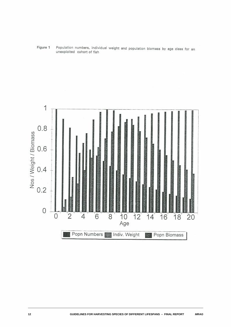
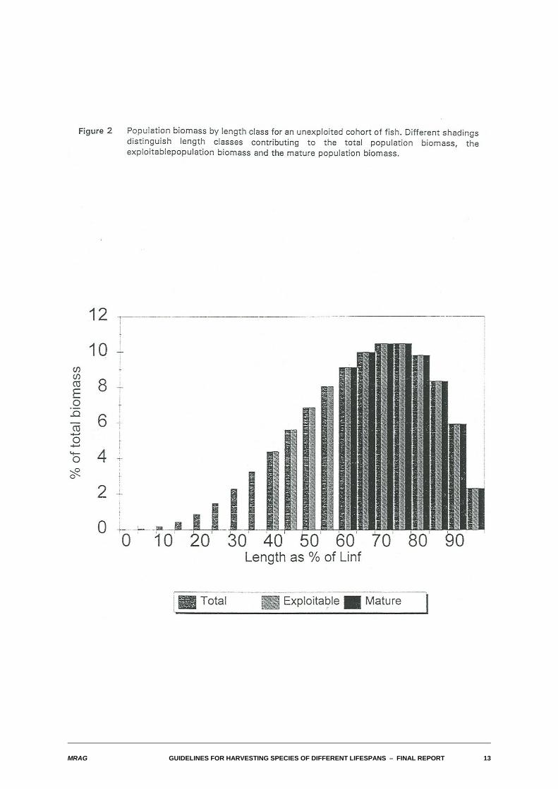
Figure 1 illustrates for nominal values of the natural mortality and growth parameters the relationshipbetween numbers, individual weight and biomass at age in a cohort of fish. Figure 2 presents essentiallysimilar information about the biomass, except now it portrays the distribution of population biomass withlength of fish as a proportion of the asymptotic maximum length. Also shown on Figure 2 are the criticalcomponents of the population: the total biomass, the exploitable biomass (of those fish with lengthsgreater than or equal to the length at first capture) and the spawning stock biomass (of those fish withlengths greater than or equal to the length at maturity).
With these preliminaries, Kirkwood et al (1994) then detailed how the equilibrium yield from a fishpopulation can be calculated. For the case where the annual recruitment (R in the equation above) isconstant, the dynamics of a cohort are exactly the same as those of the population at any one time.
12 GUIDELINES FOR HARVESTING SPECIES OF DIFFERENT LIFESPANS S FINAL REPORT MRAG
MRAG GUIDELINES FOR HARVESTING SPECIES OF DIFFERENT LIFESPANS S FINAL REPORT 13
14 GUIDELINES FOR HARVESTING SPECIES OF DIFFERENT LIFESPANS S FINAL REPORT MRAG
Allowing for a stock-recruitment relationshipIn the model as described so far, all parameters have been assumed to be constant; they are neither age-dependent nor density-dependent. We shall examine later what happens if the natural mortality rate varieswith age. For most fish populations, it is believed that by far the majority of density-dependent effectsoccur during the egg and larval stages of their life history. In consequence, most fisheries modelsincorporate all density dependence into a non-linear relationship between the spawning stock biomassand the subsequent recruitment of juvenile fish to the population. For convenience, we suppress the eggand larval stages, and assume various relationships between the average sexually mature stock biomassduring the spawning season of a year and the subsequent recruitment of fish nominally aged zero at thebeginning of the following year.
There are various possible stock-recruitment relationships that display different degrees of densitydependence. The two most frequently used stock-recruitment relationships in fisheries were proposed byBeverton and Holt (1957) and by Ricker (1954). Of these, the humped form proposed by Ricker (1954)incorporates the greatest degree of density dependence, and thus in a sense represents an extreme.Here, we have concentrated primarily on the Beverton and Holt (1957) form, which has the twinadvantages of having a very simple mathematical form and of being relatively conservative in the degreeof density dependence it attributes to the population. Some results are also given when a Ricker-typestock-recruitment relationship is assumed. In fact, for convenience and flexibility, we have actually usedin the calculations the Shepherd (1982) functional form of stock-recruitment relationship rather than theRicker form. The two can be made to be almost indistinguishable by suitable choices of parameters.
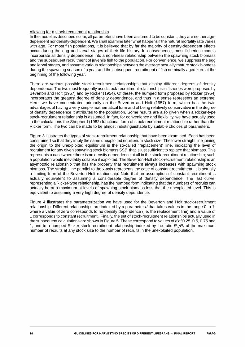
Figure 3 illustrates the types of stock-recruitment relationship that have been examined. Each has beenconstrained so that they imply the same unexploited equilibrium stock size. The lower straight line joiningthe origin to the unexploited equilibrium is the so-called "replacement" line, indicating the level ofrecruitment for any given spawning stock biomass SSB that is just sufficient to replace that biomass. Thisrepresents a case where there is no density dependence at all in the stock-recruitment relationship; sucha population would inevitably collapse if exploited. The Beverton-Holt stock-recruitment relationship is anasymptotic relationship that has the property that recruitment always increases with spawning stockbiomass. The straight line parallel to the x-axis represents the case of constant recruitment. It is actuallya limiting form of the Beverton-Holt relationship. Note that an assumption of constant recruitment isactually equivalent to assuming a considerable degree of density dependence. The last curve,representing a Ricker-type relationship, has the humped form indicating that the numbers of recruits canactually be at a maximum at levels of spawning stock biomass less that the unexploited level. This isequivalent to assuming a very high degree of density dependence.
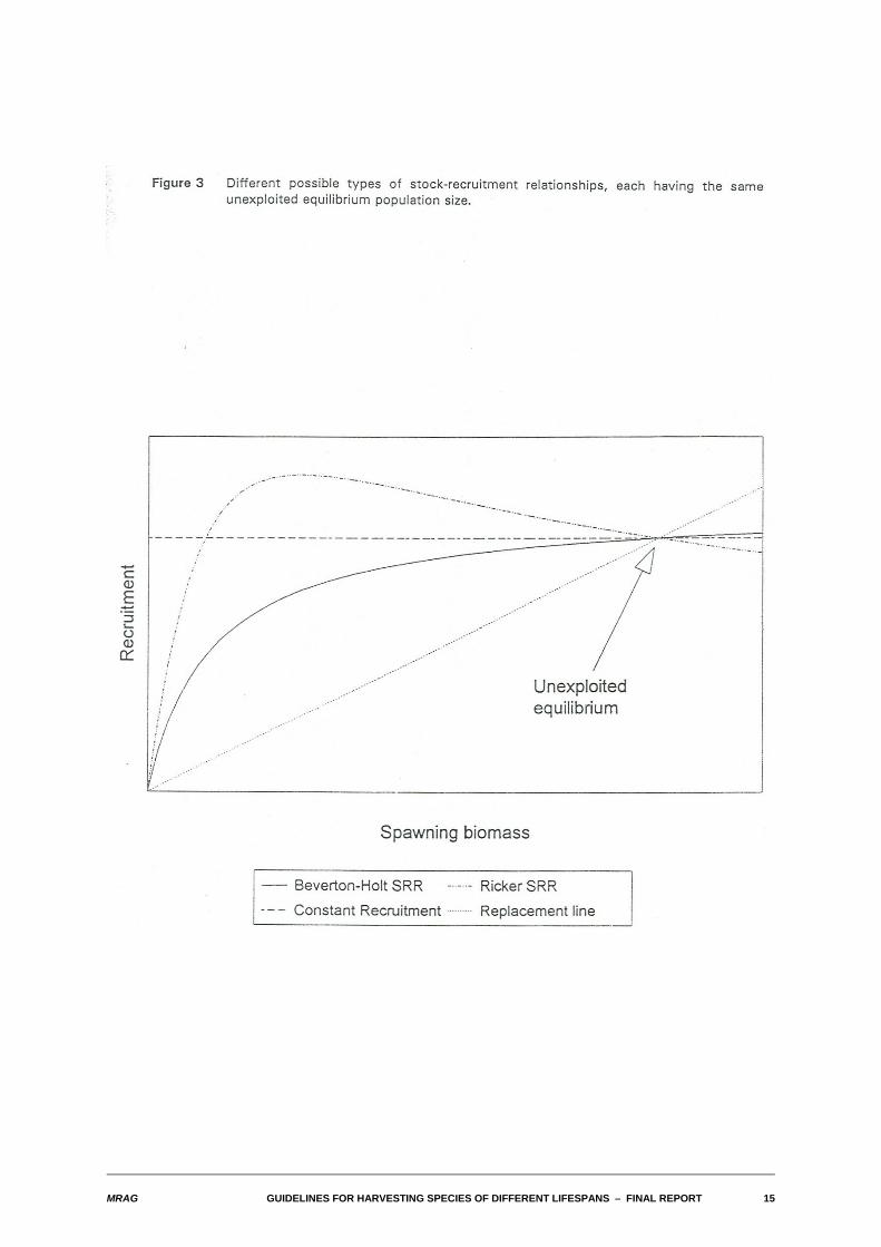
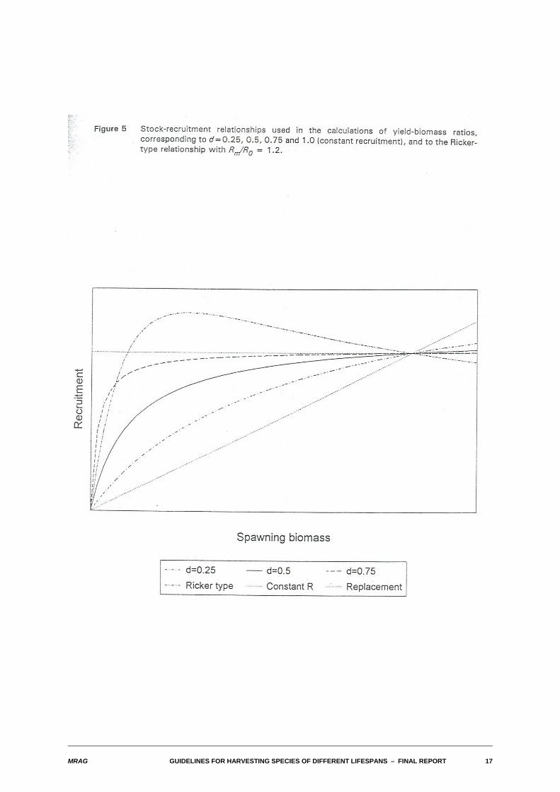
Figure 4 illustrates the parameterization we have used for the Beverton and Holt stock-recruitmentrelationship. Different relationships are indexed by a parameter d that takes values in the range 0 to 1,where a value of zero corresponds to no density dependence (i.e. the replacement line) and a value of1 corresponds to constant recruitment. Finally, the set of stock-recruitment relationships actually used inthe subsequent calculations are shown in Figure 5. These correspond to values of d of 0.25, 0.5, 0.75 and1, and to a humped Ricker stock-recruitment relationship indexed by the ratio Rm/R0 of the maximumnumber of recruits at any stock size to the number of recruits in the unexploited population.
MRAG GUIDELINES FOR HARVESTING SPECIES OF DIFFERENT LIFESPANS S FINAL REPORT 15
16 GUIDELINES FOR HARVESTING SPECIES OF DIFFERENT LIFESPANS S FINAL REPORT MRAG
MRAG GUIDELINES FOR HARVESTING SPECIES OF DIFFERENT LIFESPANS S FINAL REPORT 17
18 GUIDELINES FOR HARVESTING SPECIES OF DIFFERENT LIFESPANS S FINAL REPORT MRAG
Calculation of sustainable yields and biomassesA flexible computer program implementing the population dynamics model has been developed and usedto develop the results presented in the following sections. At its core are routines that first calculate theunexploited equilibrium population numbers and biomasses at age (or length), given specified values ofthe biological and fishery parameters. In the deterministic case, these routines then search for the fishingmortality rate that produces the maximum sustainable yield and calculate the equilibrium total andexploitable population biomass that corresponds to that level of fishing mortality. This is repeated for arange of values of the natural mortality rate, allowing the relationship between the yield-biomass ratios(MSY/ExB0 and MSY/TB0) and the natural mortality rate M to be determined. As outlined later, in mostcases this turns out to be exactly or approximately linear across species for which M/K is constant. Theapproximate constant of proportionality between the yield-biomass ratio and M is then calculated as thevalue of the yield-biomass ratio when M=1.
2.2 Typical values of parameters
As already indicated, the principal biological parameters that characterise the dynamics of the fish stockin the model we have used are the rate of natural mortality M, the growth rate K, the length at sexualmaturity Lm and the density dependence parameter d of the Beverton and Holt stock-recruitmentrelationship. There is also one important fishery-controlled parameter, the length at first capture Lc. Beinga fishery-specific parameter, the length at first capture Lc can take a wide range of values, however thereare natural inter-relationships between the various biological parameters that can be taken advantage ofto reduce the dimensionality of the problem.
The most important of these is the negative correlation between values of the natural mortality rate M andthe growth rate K. This is sufficiently strong that the ratio M/K takes only a restricted range of values. Aspart of this project, MRAG has entered into a cooperative agreement with ICLARM on the developmentof an extensive database of biological and fishery parameters for finfish species world-wide. Thisdatabase, called FISHBASE, is being jointly developed by ICLARM and FAO, and it contains, inter alia,recorded estimates of M, K, L4 and Lm for a large number of species. Through the cooperative agreementbetween MRAG and ICLARM, we have been able to gain access to a development version of FISHBASEand thus access to a wide range of estimates of the biological parameters.
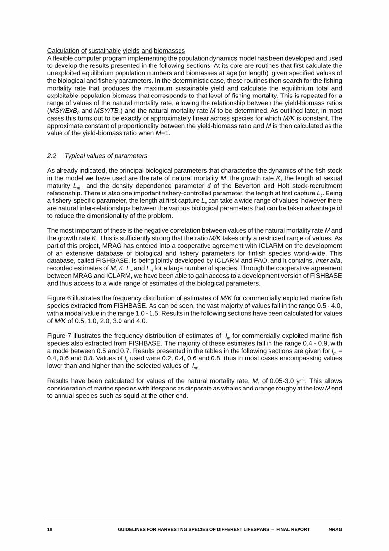
Figure 6 illustrates the frequency distribution of estimates of M/K for commercially exploited marine fishspecies extracted from FISHBASE. As can be seen, the vast majority of values fall in the range 0.5 - 4.0,with a modal value in the range 1.0 - 1.5. Results in the following sections have been calculated for valuesof M/K of 0.5, 1.0, 2.0, 3.0 and 4.0.
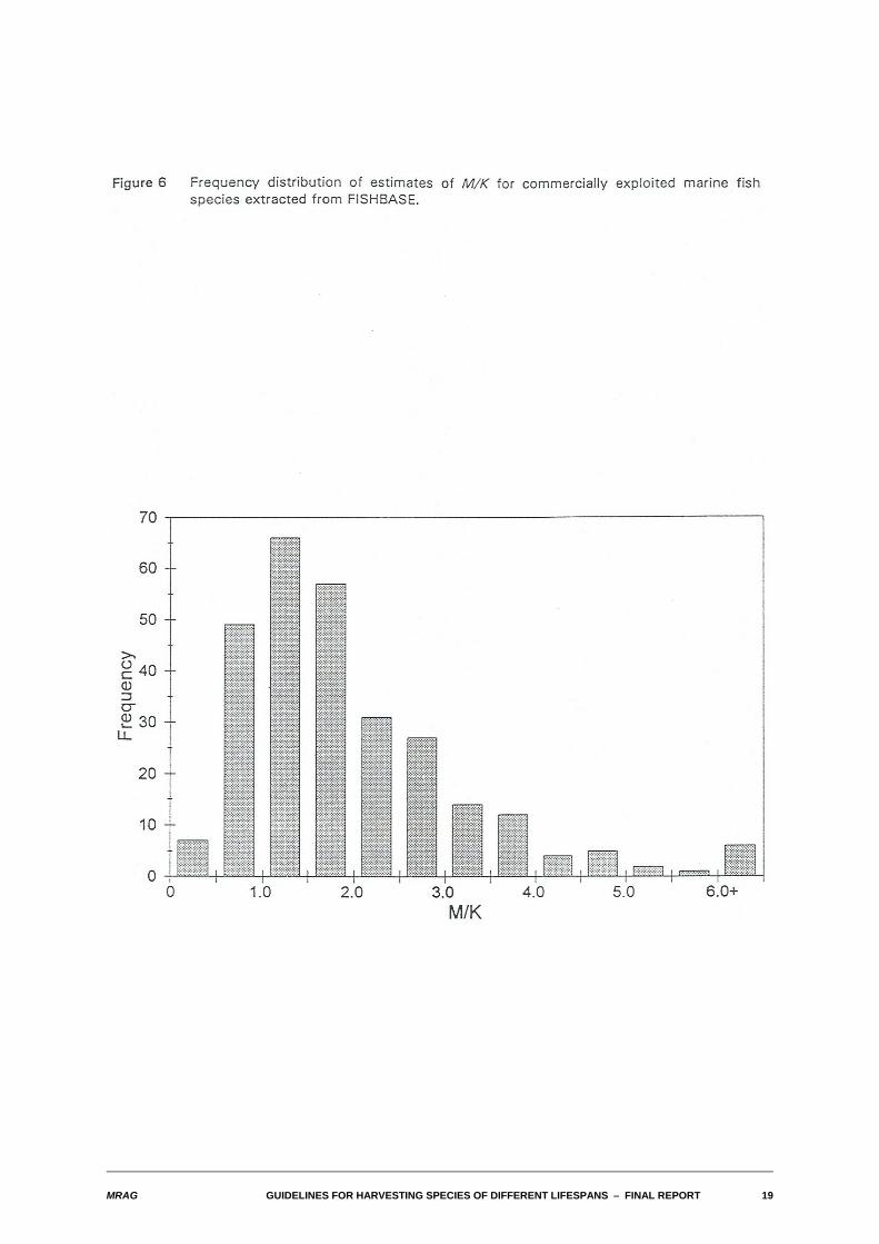
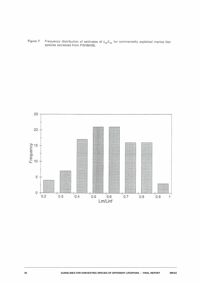
Figure 7 illustrates the frequency distribution of estimates of lm for commercially exploited marine fishspecies also extracted from FISHBASE. The majority of these estimates fall in the range 0.4 - 0.9, witha mode between 0.5 and 0.7. Results presented in the tables in the following sections are given for lm =0.4, 0.6 and 0.8. Values of lc used were 0.2, 0.4, 0.6 and 0.8, thus in most cases encompassing valueslower than and higher than the selected values of lm.
Results have been calculated for values of the natural mortality rate, M, of 0.05-3.0 yr-1. This allowsconsideration of marine species with lifespans as disparate as whales and orange roughy at the low M endto annual species such as squid at the other end.
MRAG GUIDELINES FOR HARVESTING SPECIES OF DIFFERENT LIFESPANS S FINAL REPORT 19
20 GUIDELINES FOR HARVESTING SPECIES OF DIFFERENT LIFESPANS S FINAL REPORT MRAG
MRAG GUIDELINES FOR HARVESTING SPECIES OF DIFFERENT LIFESPANS S FINAL REPORT 21
Considerable work has been undertaken recently aimed at trying to collate and characterise stock-recruitment relationships. Most notable amongst these has been the work of Mace and Sissenwine (1993),Mace (1994) and Myers et al (1994). These references contain estimated stock-recruitment relationshipsfor a number of exploited fish stocks, though they tend unsurprisingly to be mostly for stocks taken intemperate waters in developed countries. It is still a little early to attempt to identify characteristic valuesof the parameter d we have used to index the stock-recruitment relationships, so we have used values ford of 0.25, 0.5, 0.75 and 1.0, as well as a typical humped Ricker-type stock-recruitment relationship. Thesestock-recruitment relationships are those illustrated in Figure 5.
The tables produced in the next section for the cited values of biological parameters are intended to allowreaders to determine (if necessary by interpolation) the approximate maximum yield-biomass ratio andcorresponding fishing mortality rate for most combinations of estimates of biological parameters for a fishstock.
22 GUIDELINES FOR HARVESTING SPECIES OF DIFFERENT LIFESPANS S FINAL REPORT MRAG
3. Sustainable yields for constant recruitment
In this section, we present the relationships found between the deterministic equilibrium maximumsustainable yield (MSY) and the size of the exploitable biomass in a population prior to thecommencement of exploitation (ExB0). The first case considered was that in which recruitment is constantand independent of the size of the spawning stock. This simplest case was examined by Beddington andCooke (1983), and it is the only one for which any analytic progress can be made. Where recruitmentvaries according to a stock-recruitment relationship, no analytic results are available, and purely numericalmethods must be used.
As described in Kirkwood et al (1994), algebraic manipulation of the mathematical expression for the ratioMSY/ExB0 reveals that MSY/ExB0 is directly proportional to M, provided M/K and lc are kept constant. Also,the fishing mortality rate FMSY that produces the maximum sustainable yield is proportional to M for givenvalues of lc and M/K. The proportionality between the yield-biomass ratio and the natural mortality rateproposed by Gulland therefore is correct.
At first sight, this finding appears to contradict the results obtained by Beddington and Cooke (1983),whose figures suggest that the relationship between yield-biomass ratios and M is neither proportional norlinear. The difference lies in the requirements that M/K be constant, and that yield-biomass ratios beviewed as a function of lc, rather than of tc. The requirement that M/K be constant is not at all restrictive;it simply indicates that the constant of proportionality in the relationship will vary with both the value of M/Kand that of lc. Precisely the same arguments apply to the relationship between M and the ratio of MSY tounexploited total biomass (TB0), although the constants of proportionality are different, of course. Whetherin practice it is more convenient to concentrate on exploitable or total biomasses depends on which ofthese two quantities is easier to estimate.
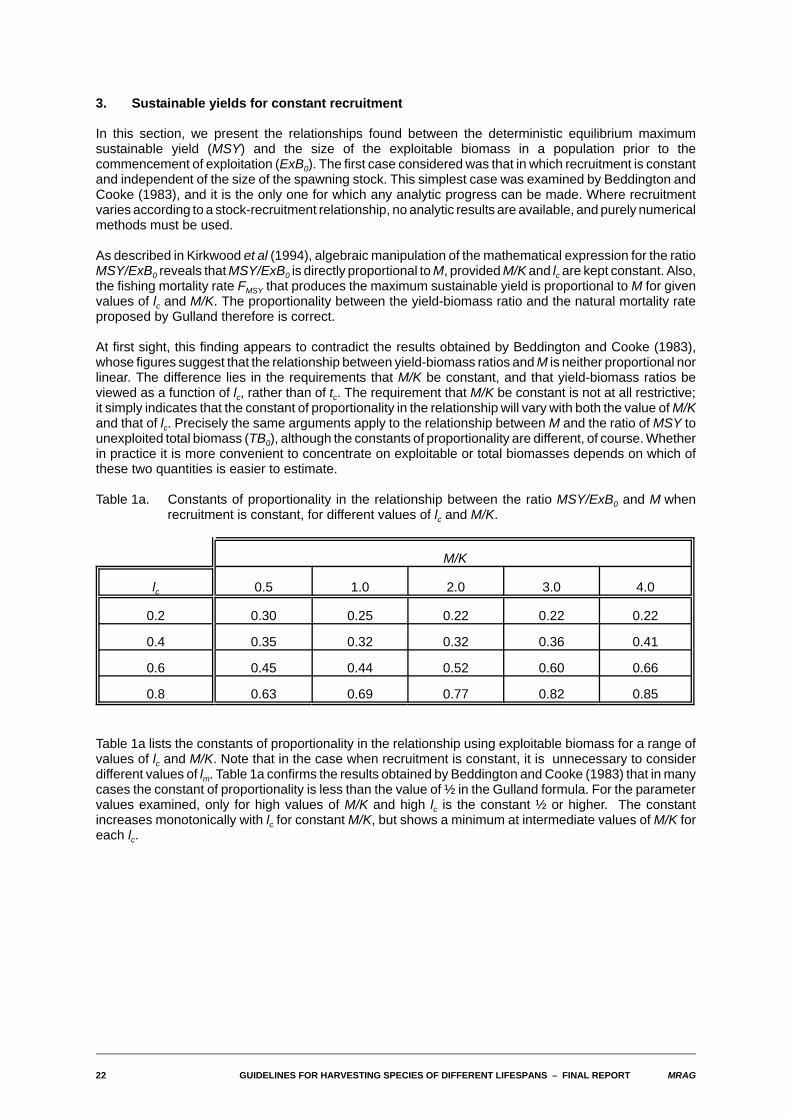
Table 1a. Constants of proportionality in the relationship between the ratio MSY/ExB0 and M whenrecruitment is constant, for different values of lc and M/K.
M/K
lc 0.5 1.0 2.0 3.0 4.0
0.2 0.30 0.25 0.22 0.22 0.22
0.4 0.35 0.32 0.32 0.36 0.41
0.6 0.45 0.44 0.52 0.60 0.66
0.8 0.63 0.69 0.77 0.82 0.85
Table 1a lists the constants of proportionality in the relationship using exploitable biomass for a range ofvalues of lc and M/K. Note that in the case when recruitment is constant, it is unnecessary to considerdifferent values of lm. Table 1a confirms the results obtained by Beddington and Cooke (1983) that in manycases the constant of proportionality is less than the value of ½ in the Gulland formula. For the parametervalues examined, only for high values of M/K and high lc is the constant ½ or higher. The constantincreases monotonically with lc for constant M/K, but shows a minimum at intermediate values of M/K foreach lc.
MRAG GUIDELINES FOR HARVESTING SPECIES OF DIFFERENT LIFESPANS S FINAL REPORT 23
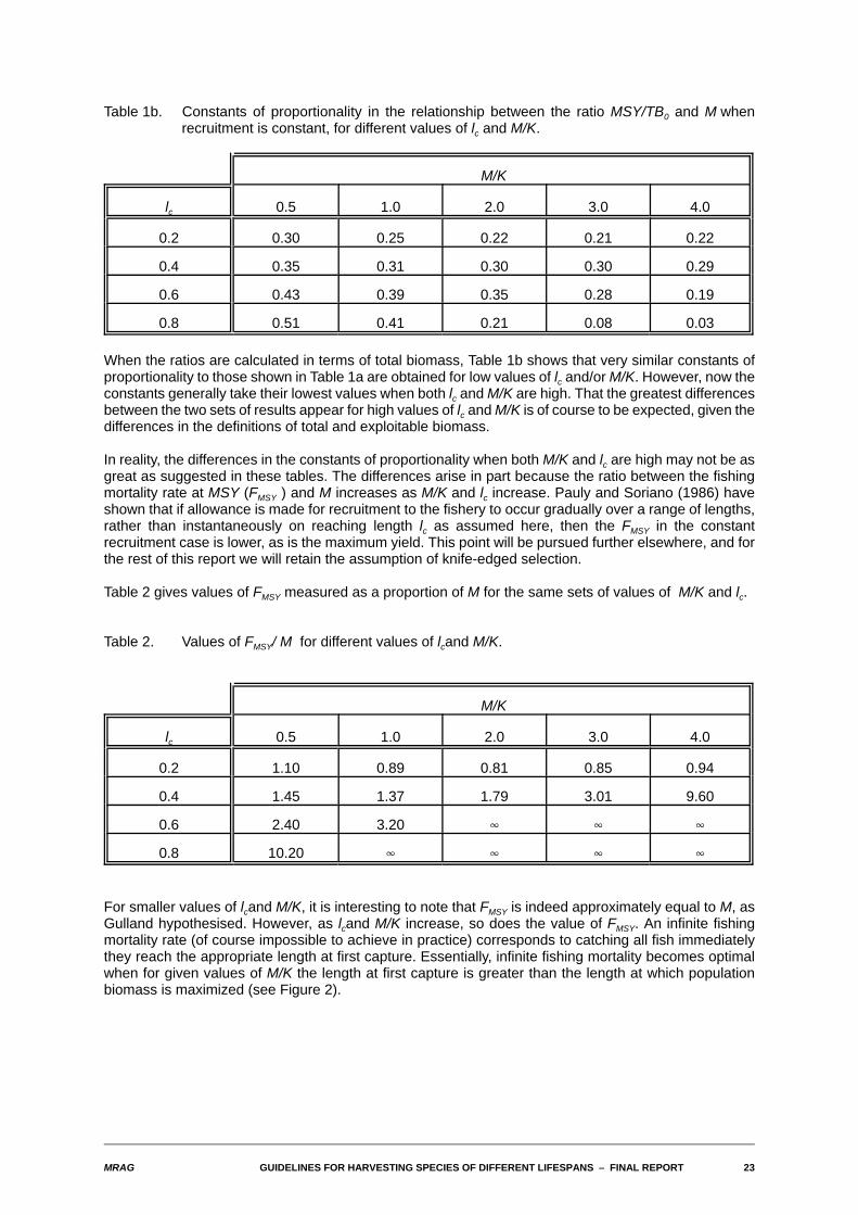
Table 1b. Constants of proportionality in the relationship between the ratio MSY/TB0 and M whenrecruitment is constant, for different values of lc and M/K.
M/K
lc 0.5 1.0 2.0 3.0 4.0
0.2 0.30 0.25 0.22 0.21 0.22
0.4 0.35 0.31 0.30 0.30 0.29
0.6 0.43 0.39 0.35 0.28 0.19
0.8 0.51 0.41 0.21 0.08 0.03
When the ratios are calculated in terms of total biomass, Table 1b shows that very similar constants ofproportionality to those shown in Table 1a are obtained for low values of lc and/or M/K. However, now theconstants generally take their lowest values when both lc and M/K are high. That the greatest differencesbetween the two sets of results appear for high values of lc and M/K is of course to be expected, given thedifferences in the definitions of total and exploitable biomass.
In reality, the differences in the constants of proportionality when both M/K and lc are high may not be asgreat as suggested in these tables. The differences arise in part because the ratio between the fishingmortality rate at MSY (FMSY ) and M increases as M/K and lc increase. Pauly and Soriano (1986) haveshown that if allowance is made for recruitment to the fishery to occur gradually over a range of lengths,rather than instantaneously on reaching length lc as assumed here, then the FMSY in the constantrecruitment case is lower, as is the maximum yield. This point will be pursued further elsewhere, and forthe rest of this report we will retain the assumption of knife-edged selection.
Table 2 gives values of FMSY measured as a proportion of M for the same sets of values of M/K and lc.
Table 2. Values of FMSY/ M for different values of lcand M/K.
M/K
lc 0.5 1.0 2.0 3.0 4.0
0.2 1.10 0.89 0.81 0.85 0.94
0.4 1.45 1.37 1.79 3.01 9.60
0.6 2.40 3.20 4 4 4
0.8 10.20 4 4 4 4
For smaller values of lcand M/K, it is interesting to note that FMSY is indeed approximately equal to M, asGulland hypothesised. However, as lcand M/K increase, so does the value of FMSY. An infinite fishingmortality rate (of course impossible to achieve in practice) corresponds to catching all fish immediatelythey reach the appropriate length at first capture. Essentially, infinite fishing mortality becomes optimalwhen for given values of M/K the length at first capture is greater than the length at which populationbiomass is maximized (see Figure 2).
24 GUIDELINES FOR HARVESTING SPECIES OF DIFFERENT LIFESPANS S FINAL REPORT MRAG
4. Allowing for a stock-recruitment relationship
4.1 Nature of relationship between yield-biomass ratio and M
Given the direct proportionality found between MSY/ExB0 and M when recruitment is constant, it istempting to hypothesise that the same relationship might hold when recruitment varies as a function of thesize of the spawning stock. This is not true, but for many biologically likely parameter combinations therelationship turns out to be very close to proportional. As in the preceding section, we will concentrateprimarily on investigating the relationships between MSY/ExB0 and M. However, we now also needconsider different values of lm. We first examine the extent of non-linearity in the relationship betweenyield-biomass ratios and M.
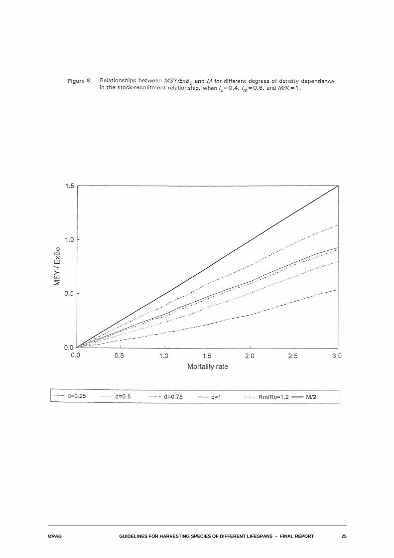
The typical result of allowing recruitment to vary with spawning stock size is seen in Figure 8. There, theempirical relationship between MSY/ExB0 and M is shown for differing degrees of density dependence inthe stock-recruitment relationship, in a typical case where lc=0.4, lm=0.6, and M/K=1. Two features areobvious. Firstly, the overall impression is that the relationship is very close to linear. Note that the apparent"waviness" of the lines is an artefact of the time-step used in the numerical calculations. The secondfeature is that the approximate slope of the lines increases as the degree of density dependence in thestock-recruitment relationship increases. This is, of course, as it should be: as the degree of densitydependence increases, the population can withstand relatively greater reductions in spawning stockbiomass corresponding to larger fishing mortalities, and thus support greater sustainable yields.
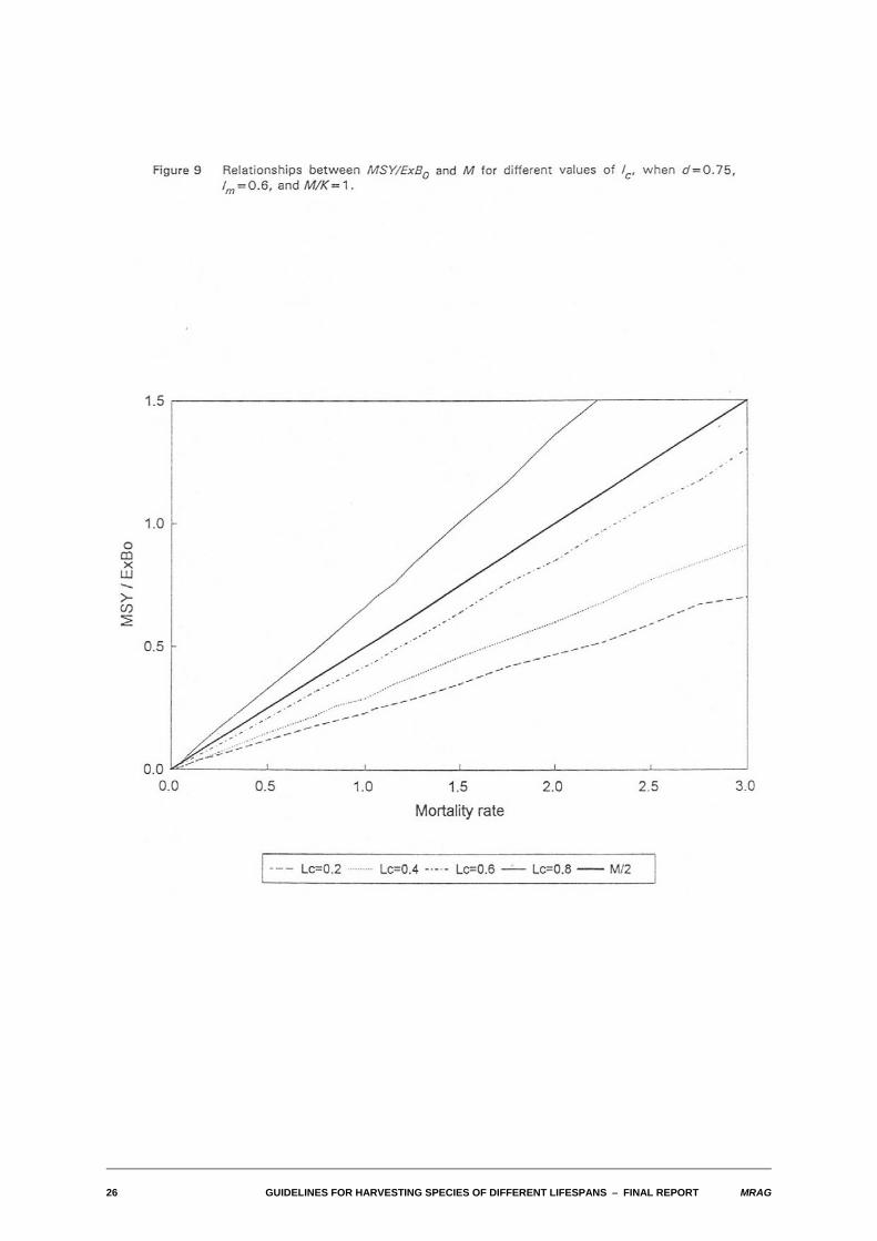
Figure 9 shows typical relationships between MSY/ExB0 and M when lc varies, with M/K set at 1.0, lm setat 0.6 and d set to 0.75. The relative proportion of the exploitable biomass that can be taken sustainablyincreases with length at first capture. Note, however, that while the proportion of exploitable biomass thatcan be taken increases with lc, the exploitable biomass itself decreases.
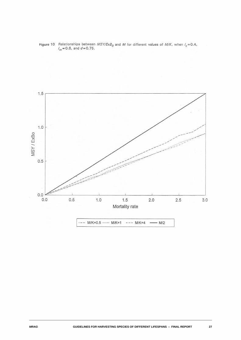
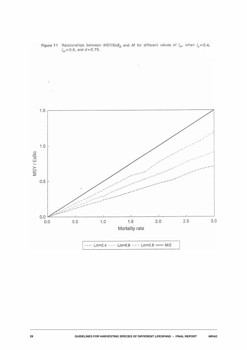
Typical relationships between MSY/ExB0 and M when M/K varies are shown in Figure 10. Somewhatsurprisingly, even over a range of M/K of 0.5-4.0 the relative proportions of exploitable biomass that canbe taken sustainably are rather similar. Figure 11 shows the effect of varying lm for the case where M/K=1.0, and lcis set equal to lm.
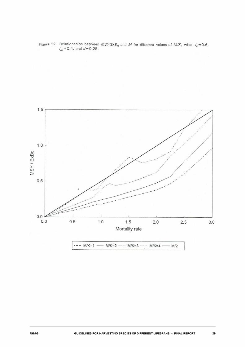
Figure 12 breaks the illusion that the departure from proportionality in the relationship between yield-biomass ratios and M is always at most minor. This figure illustrates a case where the degree of densitydependence is low (d=0.25), and where lm=0.4 and lc=0.6. For high values of M, the apparent slope of theline can increase substantially. The other unusual feature of Figure 12 is the pronounced hump in theuppermost lines for M values above around 0.75. This is not an artefact. Rather, it is a real feature arisingfrom the unusual combination of a high M/K, a length at first capture that exceeds the length at maturity,and a relatively small degree of density dependence in the stock-recruitment relation. For these valuesof M, it becomes important whether fishing during a year commences before or after the start of thespawning period and whether or not in terms of yield it is worth leaving some spawning stock to surviveand spawn an extra year.
Inspection of the full set of empirical relationships obtained indicates that substantial departures fromproportionality occur only for quite high values of M and primarily when the degree of density dependenceis small. A full investigation of the way in which species occupy different regions of parameter space isbeyond the scope of this report. However, this particular area of parameter space is biologically the mostunlikely: normally one expects that low degrees of density dependence in a stock-recruitment relation willbe associated with species that have long life-spans and therefore low mortality rates, and conversely thatspecies with nearly constant recruitment even for small spawning stock biomasses will be short-lived andfast growing.
MRAG GUIDELINES FOR HARVESTING SPECIES OF DIFFERENT LIFESPANS S FINAL REPORT 25
26 GUIDELINES FOR HARVESTING SPECIES OF DIFFERENT LIFESPANS S FINAL REPORT MRAG
MRAG GUIDELINES FOR HARVESTING SPECIES OF DIFFERENT LIFESPANS S FINAL REPORT 27
28 GUIDELINES FOR HARVESTING SPECIES OF DIFFERENT LIFESPANS S FINAL REPORT MRAG
MRAG GUIDELINES FOR HARVESTING SPECIES OF DIFFERENT LIFESPANS S FINAL REPORT 29

30 GUIDELINES FOR HARVESTING SPECIES OF DIFFERENT LIFESPANS S FINAL REPORT MRAG
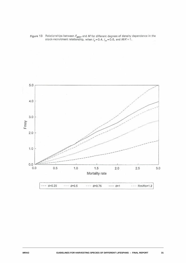
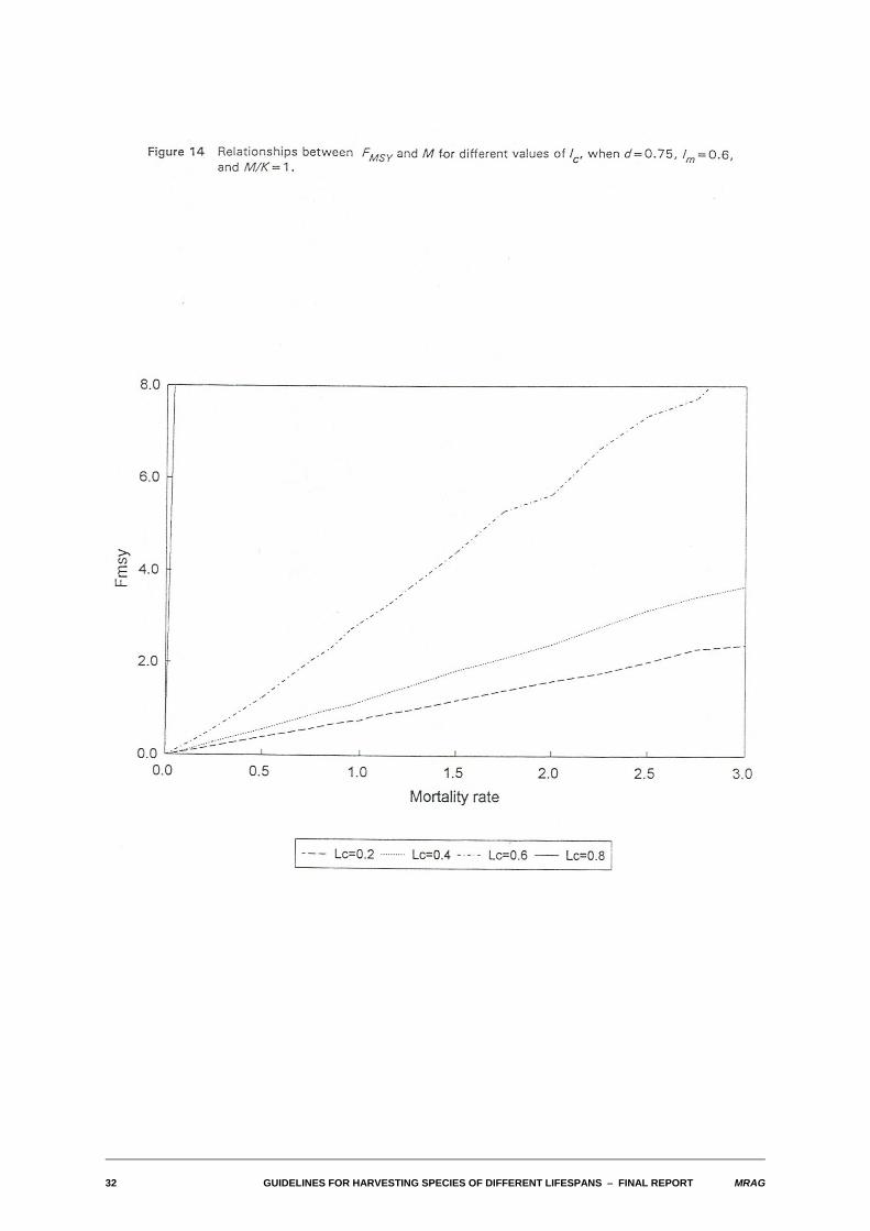
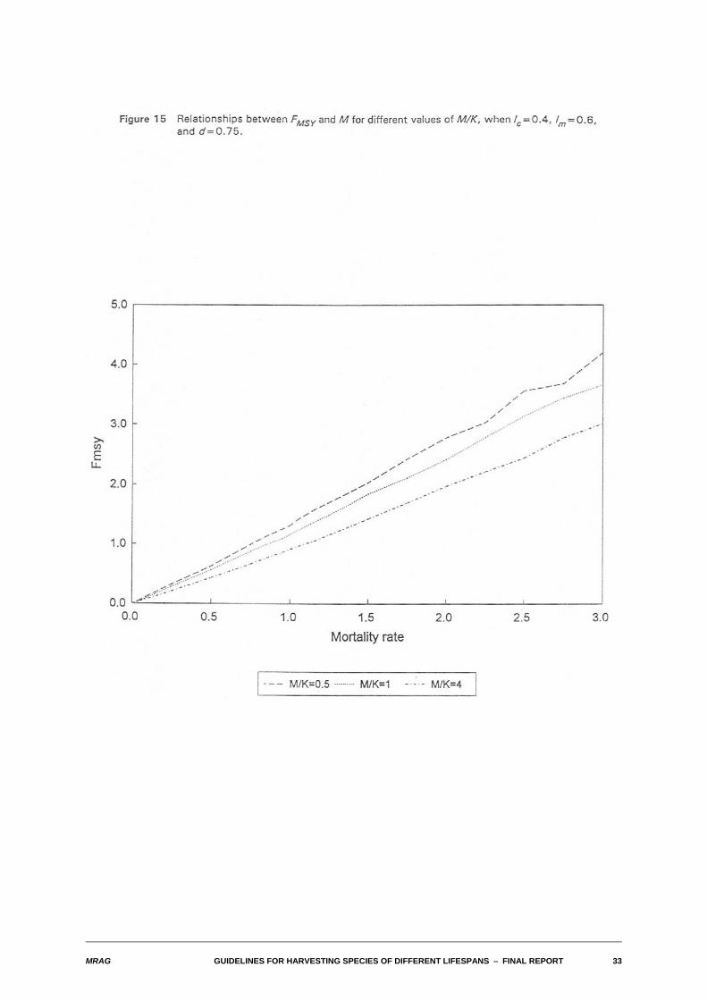
4.2 Nature of relationship between FMSY and M
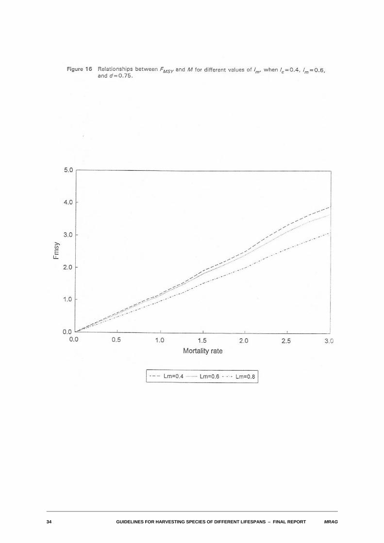
We also examined the relationships between FMSY and M for differing values of the biological and fisheryparameters. As with the yield-biomass ratios, in a wide range of cases, this relationship also turned outto be one of approximate proportionality. The relationships are illustrated in Figures 13-16 for the sameparameter combinations used in Figures 8-11.
Substantial departures from proportionality occur for the same combinations of parameters identified foryield-biomass ratios: high M, low density dependence and either high M/K or for lc larger than lm. In thosecases, FMSY tends to become infinite.
MRAG GUIDELINES FOR HARVESTING SPECIES OF DIFFERENT LIFESPANS S FINAL REPORT 31
32 GUIDELINES FOR HARVESTING SPECIES OF DIFFERENT LIFESPANS S FINAL REPORT MRAG
MRAG GUIDELINES FOR HARVESTING SPECIES OF DIFFERENT LIFESPANS S FINAL REPORT 33
34 GUIDELINES FOR HARVESTING SPECIES OF DIFFERENT LIFESPANS S FINAL REPORT MRAG

MRAG GUIDELINES FOR HARVESTING SPECIES OF DIFFERENT LIFESPANS S FINAL REPORT 35
4.3 Approximate constants of proportionality between yield-biomass ratios and M and between FMSY andM
As indicated in the methods section, given the close-to-linear relationship observed in most cases betweenthe yield-biomass ratios and M, we have taken as an estimate of the approximate constant ofproportionality the value of the yield-biomass ratio when M=1. The following tables give values of thisconstant of proportionality and of FMSY / M for the full set of values of the biological and fishery parametersinvestigated.
36 GUIDELINES FOR HARVESTING SPECIES OF DIFFERENT LIFESPANS S FINAL REPORT MRAG
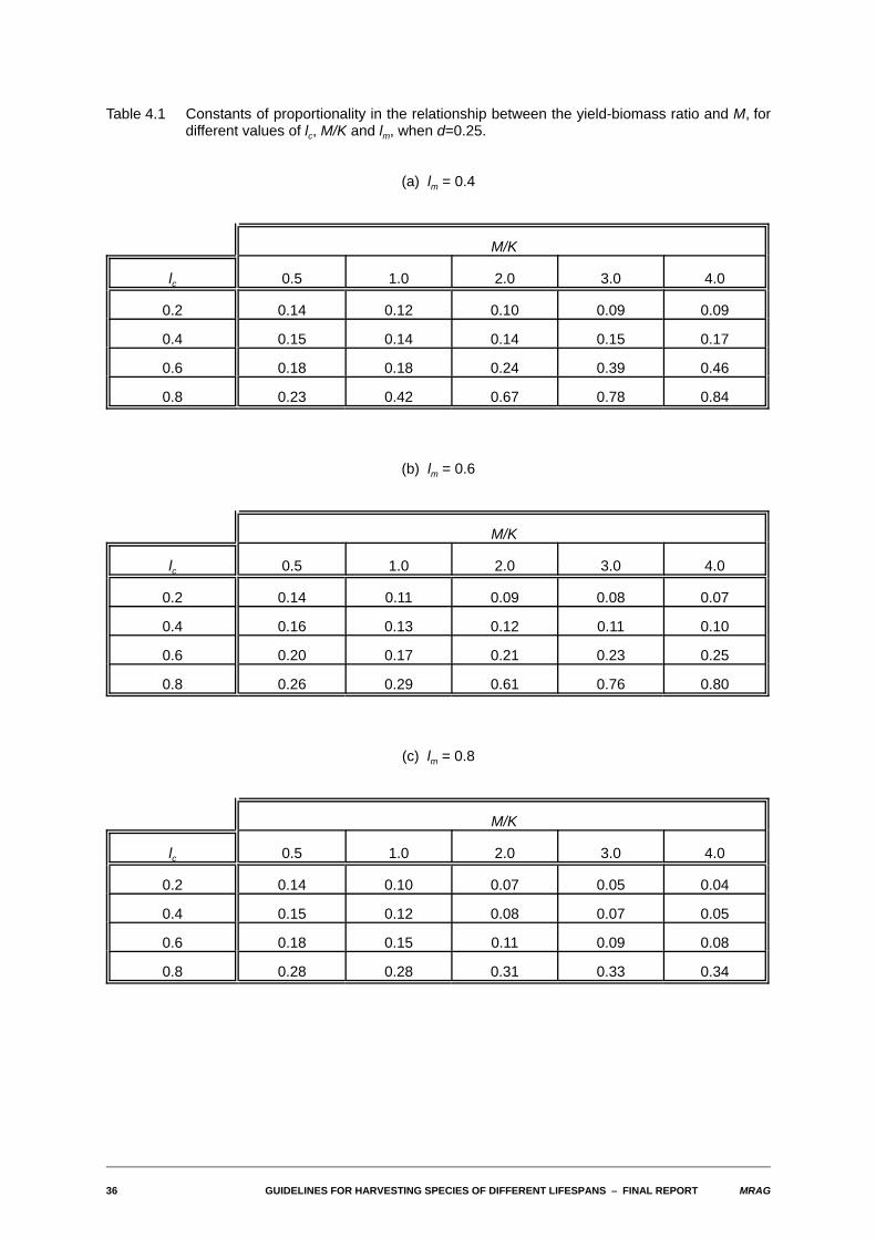
Table 4.1 Constants of proportionality in the relationship between the yield-biomass ratio and M, fordifferent values of lc, M/K and lm, when d=0.25.
(a) lm = 0.4
M/K
lc 0.5 1.0 2.0 3.0 4.0
0.2 0.14 0.12 0.10 0.09 0.09
0.4 0.15 0.14 0.14 0.15 0.17
0.6 0.18 0.18 0.24 0.39 0.46
0.8 0.23 0.42 0.67 0.78 0.84
(b) lm = 0.6
M/K
lc 0.5 1.0 2.0 3.0 4.0
0.2 0.14 0.11 0.09 0.08 0.07
0.4 0.16 0.13 0.12 0.11 0.10
0.6 0.20 0.17 0.21 0.23 0.25
0.8 0.26 0.29 0.61 0.76 0.80
(c) lm = 0.8
M/K
lc 0.5 1.0 2.0 3.0 4.0
0.2 0.14 0.10 0.07 0.05 0.04
0.4 0.15 0.12 0.08 0.07 0.05
0.6 0.18 0.15 0.11 0.09 0.08
0.8 0.28 0.28 0.31 0.33 0.34
MRAG GUIDELINES FOR HARVESTING SPECIES OF DIFFERENT LIFESPANS S FINAL REPORT 37
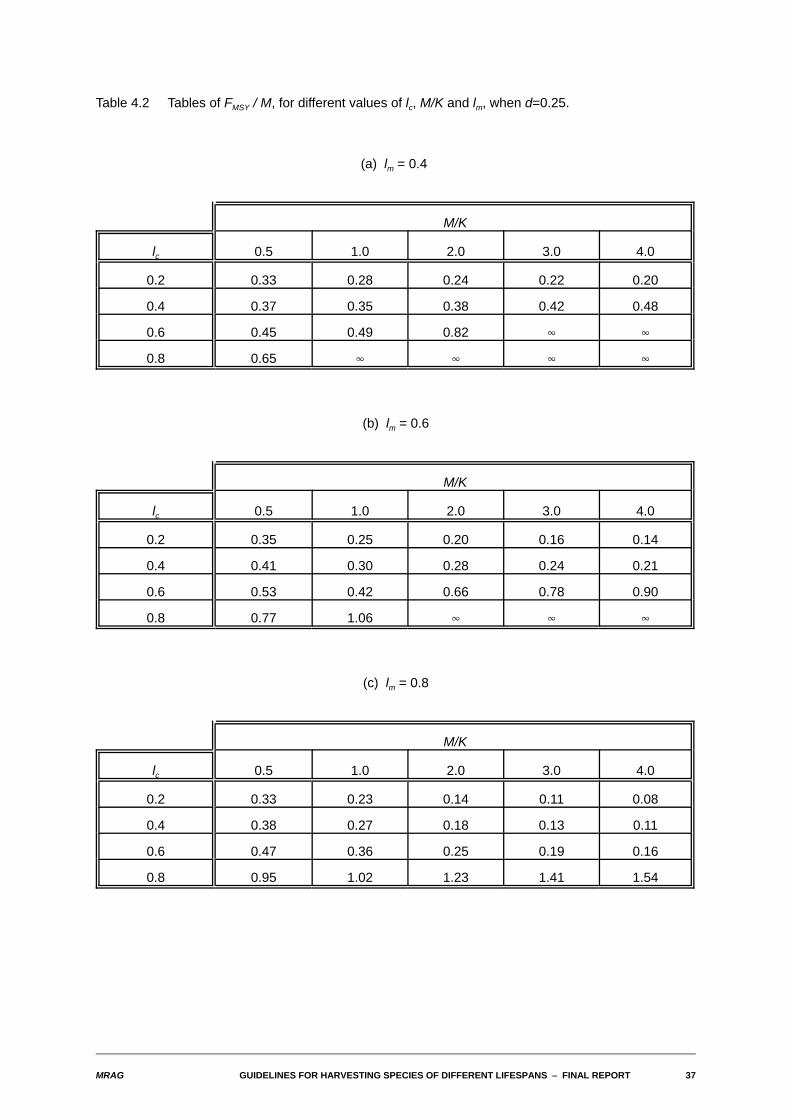
Table 4.2 Tables of FMSY / M, for different values of lc, M/K and lm, when d=0.25.
(a) lm = 0.4
M/K
lc 0.5 1.0 2.0 3.0 4.0
0.2 0.33 0.28 0.24 0.22 0.20
0.4 0.37 0.35 0.38 0.42 0.48
0.6 0.45 0.49 0.82 4 4
0.8 0.65 4 4 4 4
(b) lm = 0.6
M/K
lc 0.5 1.0 2.0 3.0 4.0
0.2 0.35 0.25 0.20 0.16 0.14
0.4 0.41 0.30 0.28 0.24 0.21
0.6 0.53 0.42 0.66 0.78 0.90
0.8 0.77 1.06 4 4 4
(c) lm = 0.8
M/K
lc 0.5 1.0 2.0 3.0 4.0
0.2 0.33 0.23 0.14 0.11 0.08
0.4 0.38 0.27 0.18 0.13 0.11
0.6 0.47 0.36 0.25 0.19 0.16
0.8 0.95 1.02 1.23 1.41 1.54

38 GUIDELINES FOR HARVESTING SPECIES OF DIFFERENT LIFESPANS S FINAL REPORT MRAG
Table 4.3 Constants of proportionality in the relationship between the yield-biomass ratio and M, fordifferent values of lc, M/K and lm, when d=0.5.
(a) lm = 0.4
M/K
lc 0.5 1.0 2.0 3.0 4.0
0.2 0.23 0.19 0.17 0.16 0.16
0.4 0.27 0.24 0.25 0.27 0.30
0.6 0.32 0.32 0.40 0.56 0.62
0.8 0.43 0.63 0.75 0.81 0.85
(b) lm = 0.6
M/K
lc 0.5 1.0 2.0 3.0 4.0
0.2 0.24 0.18 0.16 0.14 0.13
0.4 0.28 0.22 0.22 0.20 0.19
0.6 0.35 0.30 0.39 0.44 0.49
0.8 0.47 0.53 0.74 0.81 0.84
(c) lm = 0.8
M/K
lc 0.5 1.0 2.0 3.0 4.0
0.2 0.23 0.18 0.13 0.11 0.09
0.4 0.27 0.21 0.17 0.14 0.12
0.6 0.32 0.28 0.23 0.20 0.17
0.8 0.51 0.53 0.58 0.61 0.64

MRAG GUIDELINES FOR HARVESTING SPECIES OF DIFFERENT LIFESPANS S FINAL REPORT 39
Table 4.4 Tables of FMSY / M, for different values of lc, M/K and lm, when d=0.50.
(a) lm = 0.4
M/K
lc 0.5 1.0 2.0 3.0 4.0
0.2 0.68 0.57 0.49 0.46 0.44
0.4 0.82 0.79 0.91 1.17 1.62
0.6 1.07 1.24 2.63 4 4
0.8 1.74 4 4 4 4
(b) lm = 0.6
M/K
lc 0.5 1.0 2.0 3.0 4.0
0.2 0.72 0.51 0.42 0.35 0.30
0.4 0.89 0.64 0.63 0.54 0.47
0.6 1.38 1.00 2.82 4.29 5.11
0.8 2.94 6.38 4 4 4
(c) lm = 0.8
M/K
lc 0.5 1.0 2.0 3.0 4.0
0.2 0.68 0.47 0.31 0.23 0.19
0.4 0.81 0.58 0.39 0.30 0.24
0.6 1.09 0.82 0.57 0.44 0.36
0.8 3.86 4.91 6.06 6.59 6.86
40 GUIDELINES FOR HARVESTING SPECIES OF DIFFERENT LIFESPANS S FINAL REPORT MRAG
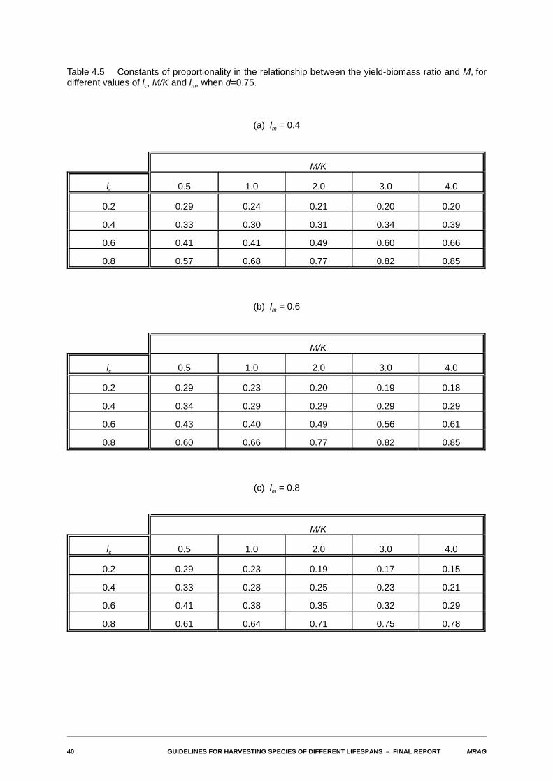
Table 4.5 Constants of proportionality in the relationship between the yield-biomass ratio and M, fordifferent values of lc, M/K and lm, when d=0.75.
(a) lm = 0.4
M/K
lc 0.5 1.0 2.0 3.0 4.0
0.2 0.29 0.24 0.21 0.20 0.20
0.4 0.33 0.30 0.31 0.34 0.39
0.6 0.41 0.41 0.49 0.60 0.66
0.8 0.57 0.68 0.77 0.82 0.85
(b) lm = 0.6
M/K
lc 0.5 1.0 2.0 3.0 4.0
0.2 0.29 0.23 0.20 0.19 0.18
0.4 0.34 0.29 0.29 0.29 0.29
0.6 0.43 0.40 0.49 0.56 0.61
0.8 0.60 0.66 0.77 0.82 0.85
(c) lm = 0.8
M/K
lc 0.5 1.0 2.0 3.0 4.0
0.2 0.29 0.23 0.19 0.17 0.15
0.4 0.33 0.28 0.25 0.23 0.21
0.6 0.41 0.38 0.35 0.32 0.29
0.8 0.61 0.64 0.71 0.75 0.78
MRAG GUIDELINES FOR HARVESTING SPECIES OF DIFFERENT LIFESPANS S FINAL REPORT 41
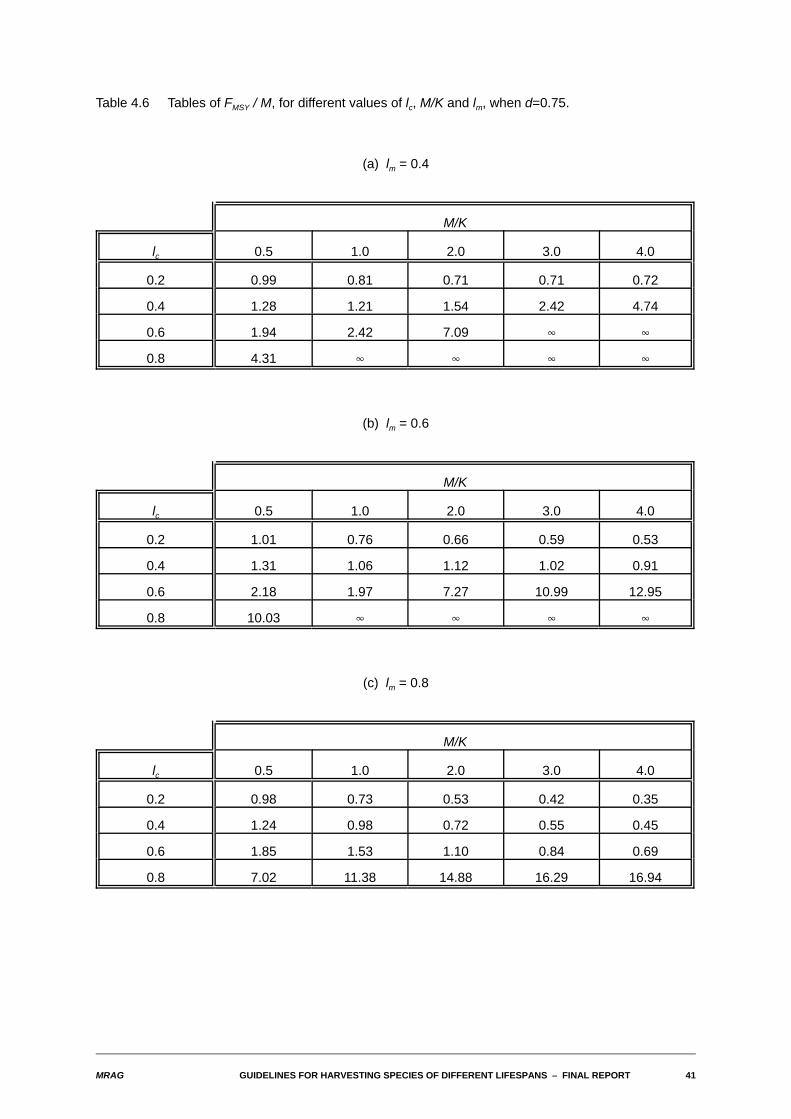
Table 4.6 Tables of FMSY / M, for different values of lc, M/K and lm, when d=0.75.
(a) lm = 0.4
M/K
lc 0.5 1.0 2.0 3.0 4.0
0.2 0.99 0.81 0.71 0.71 0.72
0.4 1.28 1.21 1.54 2.42 4.74
0.6 1.94 2.42 7.09 4 4
0.8 4.31 4 4 4 4
(b) lm = 0.6
M/K
lc 0.5 1.0 2.0 3.0 4.0
0.2 1.01 0.76 0.66 0.59 0.53
0.4 1.31 1.06 1.12 1.02 0.91
0.6 2.18 1.97 7.27 10.99 12.95
0.8 10.03 4 4 4 4
(c) lm = 0.8
M/K
lc 0.5 1.0 2.0 3.0 4.0
0.2 0.98 0.73 0.53 0.42 0.35
0.4 1.24 0.98 0.72 0.55 0.45
0.6 1.85 1.53 1.10 0.84 0.69
0.8 7.02 11.38 14.88 16.29 16.94
42 GUIDELINES FOR HARVESTING SPECIES OF DIFFERENT LIFESPANS S FINAL REPORT MRAG
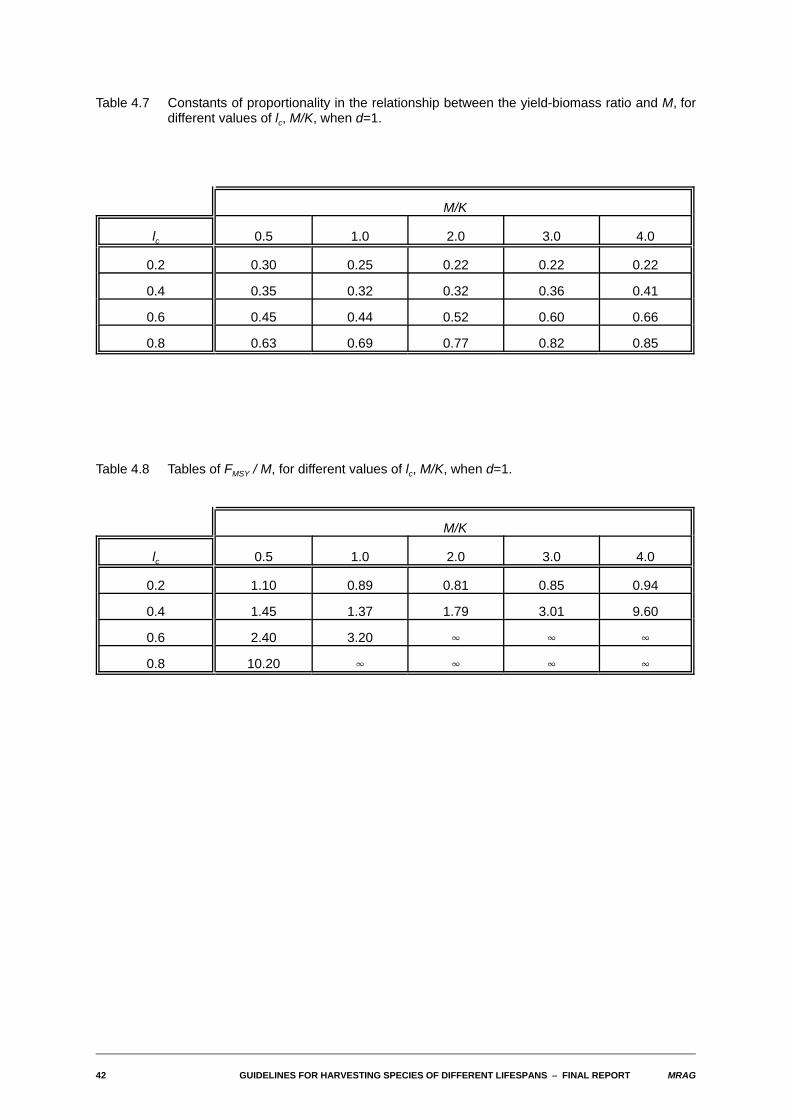
Table 4.7 Constants of proportionality in the relationship between the yield-biomass ratio and M, fordifferent values of lc, M/K, when d=1.
M/K
lc 0.5 1.0 2.0 3.0 4.0
0.2 0.30 0.25 0.22 0.22 0.22
0.4 0.35 0.32 0.32 0.36 0.41
0.6 0.45 0.44 0.52 0.60 0.66
0.8 0.63 0.69 0.77 0.82 0.85
Table 4.8 Tables of FMSY / M, for different values of lc, M/K, when d=1.
M/K
lc 0.5 1.0 2.0 3.0 4.0
0.2 1.10 0.89 0.81 0.85 0.94
0.4 1.45 1.37 1.79 3.01 9.60
0.6 2.40 3.20 4 4 4
0.8 10.20 4 4 4 4
MRAG GUIDELINES FOR HARVESTING SPECIES OF DIFFERENT LIFESPANS S FINAL REPORT 43
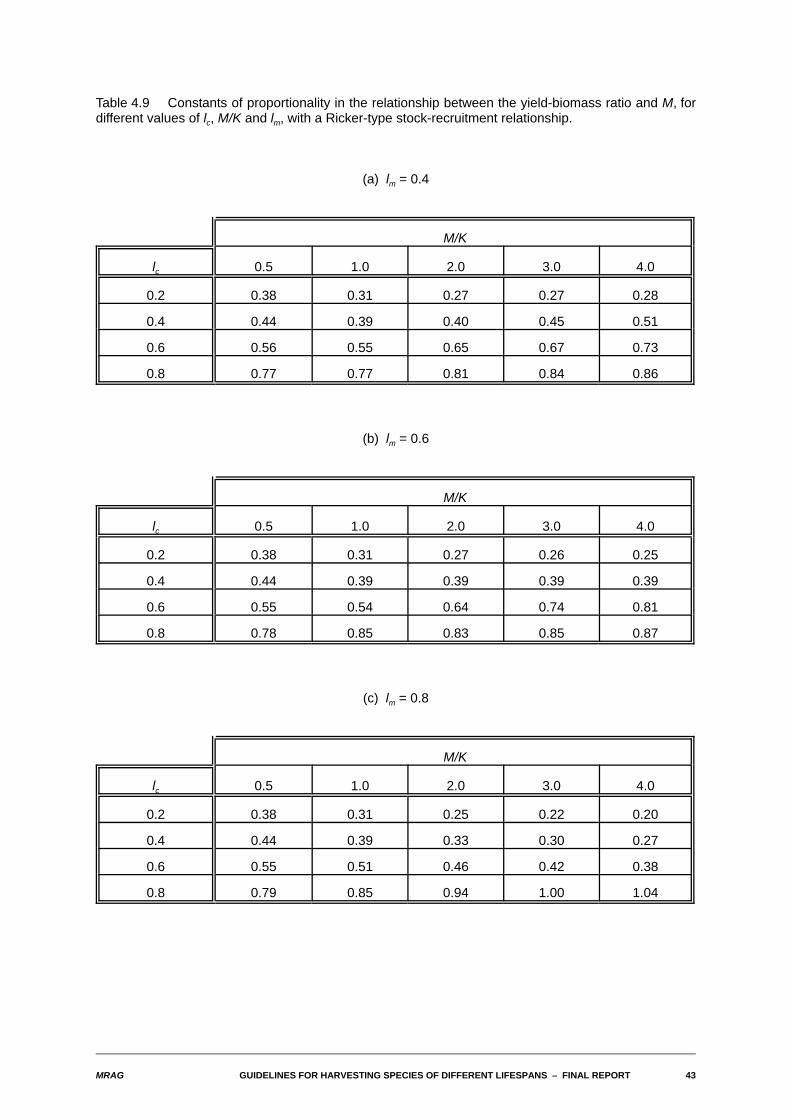
Table 4.9 Constants of proportionality in the relationship between the yield-biomass ratio and M, fordifferent values of lc, M/K and lm, with a Ricker-type stock-recruitment relationship.
(a) lm = 0.4
M/K
lc 0.5 1.0 2.0 3.0 4.0
0.2 0.38 0.31 0.27 0.27 0.28
0.4 0.44 0.39 0.40 0.45 0.51
0.6 0.56 0.55 0.65 0.67 0.73
0.8 0.77 0.77 0.81 0.84 0.86
(b) lm = 0.6
M/K
lc 0.5 1.0 2.0 3.0 4.0
0.2 0.38 0.31 0.27 0.26 0.25
0.4 0.44 0.39 0.39 0.39 0.39
0.6 0.55 0.54 0.64 0.74 0.81
0.8 0.78 0.85 0.83 0.85 0.87
(c) lm = 0.8
M/K
lc 0.5 1.0 2.0 3.0 4.0
0.2 0.38 0.31 0.25 0.22 0.20
0.4 0.44 0.39 0.33 0.30 0.27
0.6 0.55 0.51 0.46 0.42 0.38
0.8 0.79 0.85 0.94 1.00 1.04
44 GUIDELINES FOR HARVESTING SPECIES OF DIFFERENT LIFESPANS S FINAL REPORT MRAG
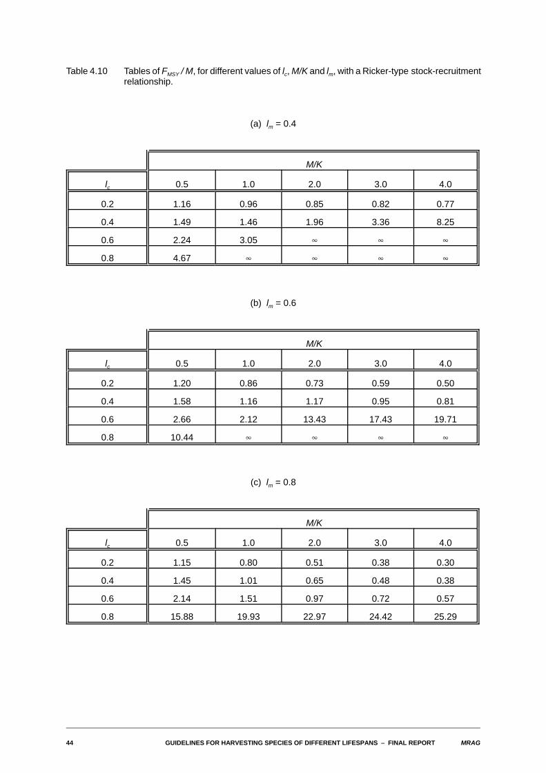
Table 4.10 Tables of FMSY / M, for different values of lc, M/K and lm, with a Ricker-type stock-recruitmentrelationship.
(a) lm = 0.4
M/K
lc 0.5 1.0 2.0 3.0 4.0
0.2 1.16 0.96 0.85 0.82 0.77
0.4 1.49 1.46 1.96 3.36 8.25
0.6 2.24 3.05 4 4 4
0.8 4.67 4 4 4 4
(b) lm = 0.6
M/K
lc 0.5 1.0 2.0 3.0 4.0
0.2 1.20 0.86 0.73 0.59 0.50
0.4 1.58 1.16 1.17 0.95 0.81
0.6 2.66 2.12 13.43 17.43 19.71
0.8 10.44 4 4 4 4
(c) lm = 0.8
M/K
lc 0.5 1.0 2.0 3.0 4.0
0.2 1.15 0.80 0.51 0.38 0.30
0.4 1.45 1.01 0.65 0.48 0.38
0.6 2.14 1.51 0.97 0.72 0.57
0.8 15.88 19.93 22.97 24.42 25.29
MRAG GUIDELINES FOR HARVESTING SPECIES OF DIFFERENT LIFESPANS S FINAL REPORT 45
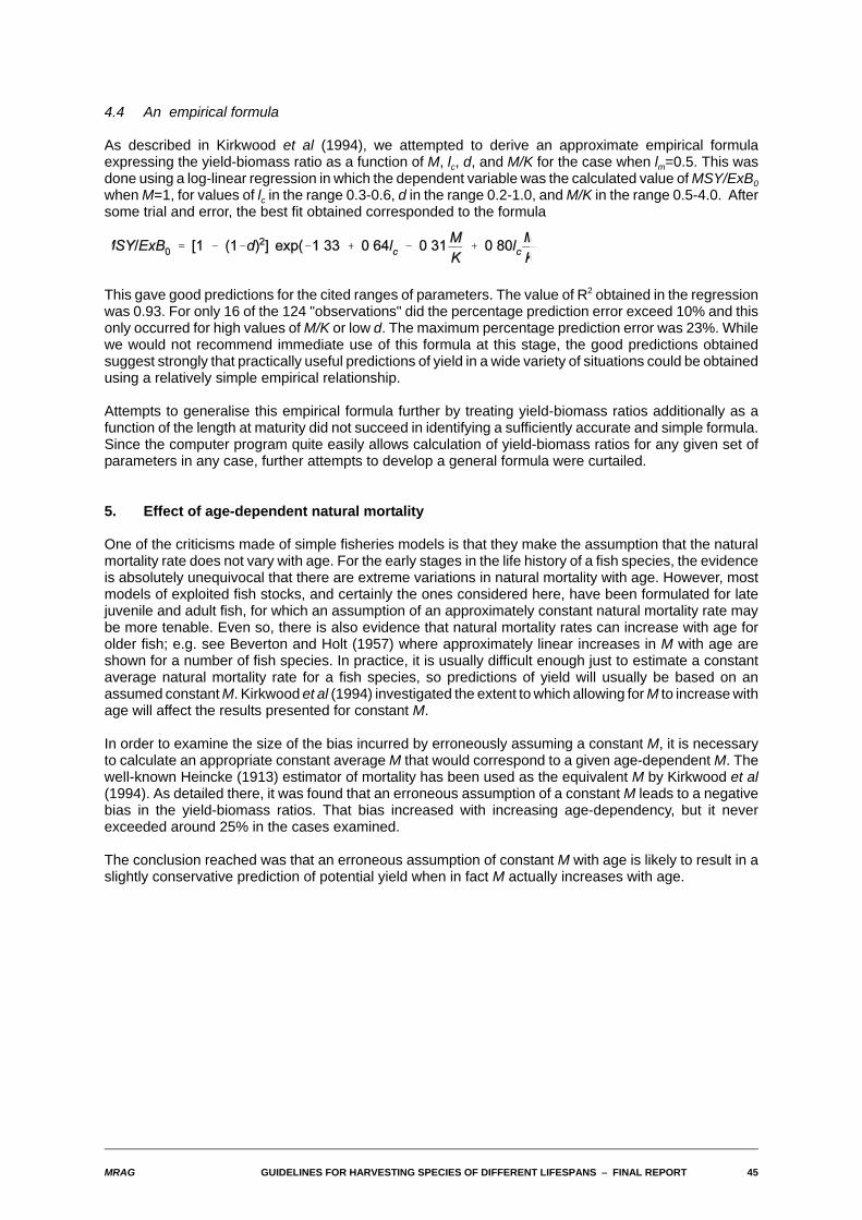
4.4 An empirical formula
As described in Kirkwood et al (1994), we attempted to derive an approximate empirical formulaexpressing the yield-biomass ratio as a function of M, lc, d, and M/K for the case when lm=0.5. This wasdone using a log-linear regression in which the dependent variable was the calculated value of MSY/ExB0when M=1, for values of lc in the range 0.3-0.6, d in the range 0.2-1.0, and M/K in the range 0.5-4.0. Aftersome trial and error, the best fit obtained corresponded to the formula
This gave good predictions for the cited ranges of parameters. The value of R2 obtained in the regressionwas 0.93. For only 16 of the 124 "observations" did the percentage prediction error exceed 10% and thisonly occurred for high values of M/K or low d. The maximum percentage prediction error was 23%. Whilewe would not recommend immediate use of this formula at this stage, the good predictions obtainedsuggest strongly that practically useful predictions of yield in a wide variety of situations could be obtainedusing a relatively simple empirical relationship.
Attempts to generalise this empirical formula further by treating yield-biomass ratios additionally as afunction of the length at maturity did not succeed in identifying a sufficiently accurate and simple formula.Since the computer program quite easily allows calculation of yield-biomass ratios for any given set ofparameters in any case, further attempts to develop a general formula were curtailed.
5. Effect of age-dependent natural mortality
One of the criticisms made of simple fisheries models is that they make the assumption that the naturalmortality rate does not vary with age. For the early stages in the life history of a fish species, the evidenceis absolutely unequivocal that there are extreme variations in natural mortality with age. However, mostmodels of exploited fish stocks, and certainly the ones considered here, have been formulated for latejuvenile and adult fish, for which an assumption of an approximately constant natural mortality rate maybe more tenable. Even so, there is also evidence that natural mortality rates can increase with age forolder fish; e.g. see Beverton and Holt (1957) where approximately linear increases in M with age areshown for a number of fish species. In practice, it is usually difficult enough just to estimate a constantaverage natural mortality rate for a fish species, so predictions of yield will usually be based on anassumed constant M. Kirkwood et al (1994) investigated the extent to which allowing for M to increase withage will affect the results presented for constant M.
In order to examine the size of the bias incurred by erroneously assuming a constant M, it is necessaryto calculate an appropriate constant average M that would correspond to a given age-dependent M. Thewell-known Heincke (1913) estimator of mortality has been used as the equivalent M by Kirkwood et al(1994). As detailed there, it was found that an erroneous assumption of a constant M leads to a negativebias in the yield-biomass ratios. That bias increased with increasing age-dependency, but it neverexceeded around 25% in the cases examined.
The conclusion reached was that an erroneous assumption of constant M with age is likely to result in aslightly conservative prediction of potential yield when in fact M actually increases with age.
46 GUIDELINES FOR HARVESTING SPECIES OF DIFFERENT LIFESPANS S FINAL REPORT MRAG
6. The special case of very short-lived species
On the surface, the results presented apply equally for all values of M. However, we have already seenthat the proportional relationship between yield-biomass ratios and M can break down for high M whenrecruitment is not constant. The argument for treating at least some very short-lived species as specialcases is unanswerable when one considers annual species like squid, which die immediately afterspawning. Such species can be considered to present extreme cases of age-dependent natural mortality:M is effectively infinite for all ages above the age at maturity.
The difficulty that occurs is not that any of the preceding calculations are incorrect, but rather that thevalues calculated for the exploitable or total biomass in an virgin population using the standard methodsno longer correspond to anything really measurable.
The biomasses as calculated both here and in Kirkwood et al (1994) actually represent an average valuethroughout a year. When M is relatively small, these biomasses really are approximately constantthroughout the year, and it is reasonable to treat an estimate of abundance in an unexploited populationmade at virtually any time throughout a year as an acceptable estimate of the annual average biomass.As M increases (and thus lifespan decreases), however, the population biomass can vary considerablythroughout the year. For annual species not only do these biomasses vary considerably throughout theyear for ages up to the age at maturity, but they are zero for the remainder of the year. This means thatinterpretation and estimation of average biomasses throughout the year are rather difficult.
In such circumstances, it is more realistic to examine ratios of yield to the biomass in an unexploitedpopulation at time tc (i.e. at the start of what would be the fishing season in an exploited stock). Apart frombeing much more easily interpretable, this biomass has the additional virtue of being practicallymeasurable, e.g. by pre-season surveys of abundance or retrospectively via within-season stockassessments. As usual, there is a cost to pay. Yield-biomass ratios and values of FMSY are perfectly welldefined when using this new measure of exploitable biomass. However, the close-to-proportionalrelationship between yield-biomass ratios and M for species with the same lc and M/K unfortunately nolonger holds.
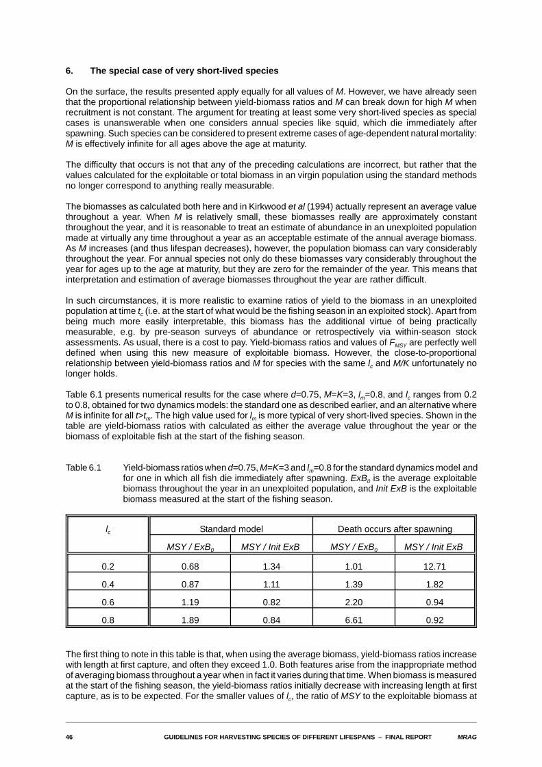
Table 6.1 presents numerical results for the case where d=0.75, M=K=3, lm=0.8, and lc ranges from 0.2to 0.8, obtained for two dynamics models: the standard one as described earlier, and an alternative whereM is infinite for all t>tm. The high value used for lm is more typical of very short-lived species. Shown in thetable are yield-biomass ratios with calculated as either the average value throughout the year or thebiomass of exploitable fish at the start of the fishing season.
Table 6.1 Yield-biomass ratios when d=0.75, M=K=3 and lm=0.8 for the standard dynamics model andfor one in which all fish die immediately after spawning. ExB0 is the average exploitablebiomass throughout the year in an unexploited population, and Init ExB is the exploitablebiomass measured at the start of the fishing season.
lc Standard model Death occurs after spawning
MSY / ExB0 MSY / Init ExB MSY / ExB0 MSY / Init ExB
0.2 0.68 1.34 1.01 12.71
0.4 0.87 1.11 1.39 1.82
0.6 1.19 0.82 2.20 0.94
0.8 1.89 0.84 6.61 0.92
The first thing to note in this table is that, when using the average biomass, yield-biomass ratios increasewith length at first capture, and often they exceed 1.0. Both features arise from the inappropriate methodof averaging biomass throughout a year when in fact it varies during that time. When biomass is measuredat the start of the fishing season, the yield-biomass ratios initially decrease with increasing length at firstcapture, as is to be expected. For the smaller values of lc, the ratio of MSY to the exploitable biomass at

MRAG GUIDELINES FOR HARVESTING SPECIES OF DIFFERENT LIFESPANS S FINAL REPORT 47
the start of the season can still be substantially greater than 1.0, especially when death occurs afterspawning. This may seem somewhat bizarre, but it simply reflects the fact that fishing has started wellbefore the population has reached its maximum biomass for the year.
Comparing the results across dynamics models, the yield-biomass ratios are considerably higher whenthe fish die immediately after spawning, particularly for low values of lc. This is because even for this highM, there are sufficiently many survivors into a second year to influence the size of the exploitable biomassat the start of the season. There are no survivors to a second year if death occurs after spawning.
The tables of constants of proportionality presented in sections 3 and 4 were calculated for M=1, a valueof M for which there is not that much difference between the two methods of calculating exploitablebiomasses. The findings in this section indicate that for larger M problems do arise. In the following sectionwe present estimates of yield-biomass ratios for selected species from FISHBASE for which estimatesof all or most of the biological and fishery parameters are available. A number of these species are short-lived tropical species. According we include estimates of yield-biomass ratios calculated in both ways inthe results.
48 GUIDELINES FOR HARVESTING SPECIES OF DIFFERENT LIFESPANS S FINAL REPORT MRAG
7. Estimates of yield-biomass ratios and FMSY for selected species
The FISHBASE database being jointly developed by ICLARM and FAO is intended to be, on release, themost up-to-date and comprehensive collation of both biological and fisheries information existinganywhere. The decision by MRAG to become a collaborator was in considerable part taken with a viewthat information from that database could be used to obtain direct estimates of yield-biomass ratios andoptimum fishing mortality rates for a wide range of commercially important marine species, particularlythose found in the tropics and fished by developing countries. As is well known, it is for these species thatit is most difficult to obtain appropriate information.
The table of estimates that concludes this section has been assembled by extracting estimates of the citedparameters from the database and then using the computer program developed during this project toperform the necessary calculations. It must be emphasised, however, that these estimates should beconsidered as preliminary only, for a number of reasons. First, the FISHBASE database is still underdevelopment, and the version we have used to extract information is still preliminary. The final versionreleased will not only cover more species and contain more information about species already in thedatabase, but will also be subject to more rigorous checking. That said, however, the database isintended to record faithfully biological and fisheries information as recorded in the literature. No attempthas been made to review the likely accuracy of that information. Before estimates of yield-biomass ratioswere to be used for management purposes for a particular species, it would be vital to undertake such areview. In the time available, we have not attempted to do so for the species in the table, although acouple of species have been omitted where the recorded biological parameters are clearly quiteinconsistent.
The version of the database used has a total of 1200 fields available to record quantitative and qualitativeinformation for each species, and information of some sort is available for nearly 9000 different speciesof the roughly 24000 fish species existing in the world. We firstly restricted attention to commerciallyexploited or potentially exploitable marine species. In terms of the biological parameters needed, fieldsare available in the database records for a species to contain estimates of M, K, L4, to,and lm. Theprincipal fishery parameter needed is lc, the length at first capture. This is actually not recorded explicitly,but a related parameter, lcom the "common" length in the catch, is recorded. The true value of lc clearly willbe less than lcom, but by how much is unclear.
Ideally, one would seek to select stocks of a species for which appropriately calculated estimates of allthese parameters are recorded using consistent units. In practice, this only occurred very rarely in thedevelopment version of the database available. The most commonly available parameter estimates arefor M, K, and L4, and in the table below we have required that estimates of those three parameters areavailable for a specified stock of a species before it can be included in the table. Where correspondingestimates of to are recorded, these have been used, but otherwise to was taken to be zero. Where multipleestimates of parameters exist on the database, a judgement was made as to which were the most reliable.Estimates of lm (relative to L4) were rather less frequently available for the same stock and species. If aconsistent estimate of lmwas available for other stocks of the same species, or if necessary for relatedspecies, this has been used in the table below for important tropical species. In a few cases indicated witha superscript asterisk, a value of 0.5 has been assumed for lm.
Values of lc were chosen according to the following rule:
If an estimate of lcom exists and lcom < 0.8 lm, then lc=lcom,
Otherwise, lc=0.8 lm.
This is to a large extent arbitrary, but it is relatively rare for fish not to be exploited before they becomemature, and the above rule ensures that is avoided.
The database does not include any estimates of potential stock-recruitment relationships. As alreadynoted, estimates of stock-recruitment parameters have been gathered by Myers et al (1994), but theseare mainly for species exploited in developed countries. In the table below, we have included estimatesof the parameter d of the Beverton-Holt stock-recruitment relationship where it can be estimated for aspecies and stock, but otherwise, we have calculated yield-biomass ratios and fishing mortality rates fora Beverton-Holt relationship with d=0.5 and for a Ricker-type relationship with Rm/R0=1.2, taking theseto represent relatively low levels of density dependence. In these cases, yield-biomass ratios and FMSY
MRAG GUIDELINES FOR HARVESTING SPECIES OF DIFFERENT LIFESPANS S FINAL REPORT 49
estimates are given as a range of values, the lower end corresponding to the Beverton-Holt relationship,and the upper end to the Ricker-type relationship, and no specific value of d is recorded.
When these results were first calculated, we had initially calculated ranges of estimates corresponding toBeverton-Holt parameters of d=0.5 and d=1.0, the latter corresponding to a constant recruitment. Whilethe yield-biomass ratios are often not that different for the constant recruitment and the Ricker-typerelationship (those for the Ricker-type are usually higher), the values of FMSY for the constant recruitmentrelationship can often be either very large or infinite. This only occurs because there is no penalty forreducing the spawning stock biomass to very low levels. Basing management on such an extremeassumption is clearly not conservative, so we have opted to base upper ranges on a Ricker-typerelationship.
One other biological parameter needed in the computer program is the exponent b in the length-weightrelationship L%Wb. In some cases, this was not recorded in FISHBASE, in which case we have assumedthe conventional value of 3 for b.
As indicated in section 6, the difficulties that arise in interpretation of yield-biomass ratios for high M valuesrequire that we include in the table ratios of MSY to both measures of initial exploitable biomass: ExB0,which is the average exploitable biomass in an unfished population throughout the year, and Init ExB,which is the exploitable biomass in an unfished population estimated at the start of the fishing season.
Table 7.1 lists estimates obtained for a total of 53 commercially exploitable marine species.
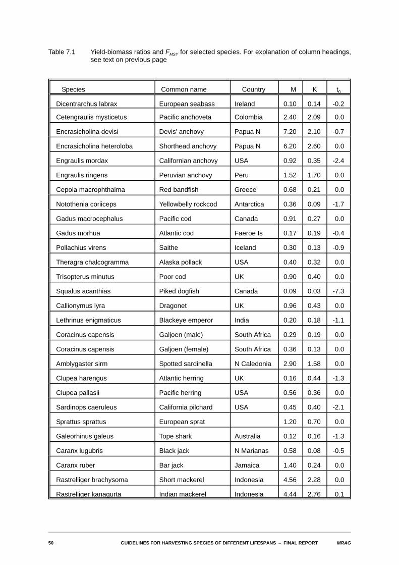
50 GUIDELINES FOR HARVESTING SPECIES OF DIFFERENT LIFESPANS S FINAL REPORT MRAG
Table 7.1 Yield-biomass ratios and FMSY for selected species. For explanation of column headings,see text on previous page
Species Common name Country M K t0
Dicentrarchus labrax European seabass Ireland 0.10 0.14 -0.2
Cetengraulis mysticetus Pacific anchoveta Colombia 2.40 2.09 0.0
Encrasicholina devisi Devis' anchovy Papua N 7.20 2.10 -0.7
Encrasicholina heteroloba Shorthead anchovy Papua N 6.20 2.60 0.0
Engraulis mordax Californian anchovy USA 0.92 0.35 -2.4
Engraulis ringens Peruvian anchovy Peru 1.52 1.70 0.0
Cepola macrophthalma Red bandfish Greece 0.68 0.21 0.0
Notothenia coriiceps Yellowbelly rockcod Antarctica 0.36 0.09 -1.7
Gadus macrocephalus Pacific cod Canada 0.91 0.27 0.0
Gadus morhua Atlantic cod Faeroe Is 0.17 0.19 -0.4
Pollachius virens Saithe Iceland 0.30 0.13 -0.9
Theragra chalcogramma Alaska pollack USA 0.40 0.32 0.0
Trisopterus minutus Poor cod UK 0.90 0.40 0.0
Squalus acanthias Piked dogfish Canada 0.09 0.03 -7.3
Callionymus lyra Dragonet UK 0.96 0.43 0.0
Lethrinus enigmaticus Blackeye emperor India 0.20 0.18 -1.1
Coracinus capensis Galjoen (male) South Africa 0.29 0.19 0.0
Coracinus capensis Galjoen (female) South Africa 0.36 0.13 0.0
Amblygaster sirm Spotted sardinella N Caledonia 2.90 1.58 0.0
Clupea harengus Atlantic herring UK 0.16 0.44 -1.3
Clupea pallasii Pacific herring USA 0.56 0.36 0.0
Sardinops caeruleus California pilchard USA 0.45 0.40 -2.1
Sprattus sprattus European sprat 1.20 0.70 0.0
Galeorhinus galeus Tope shark Australia 0.12 0.16 -1.3
Caranx lugubris Black jack N Marianas 0.58 0.08 -0.5
Caranx ruber Bar jack Jamaica 1.40 0.24 0.0
Rastrelliger brachysoma Short mackerel Indonesia 4.56 2.28 0.0
Rastrelliger kanagurta Indian mackerel Indonesia 4.44 2.76 0.1
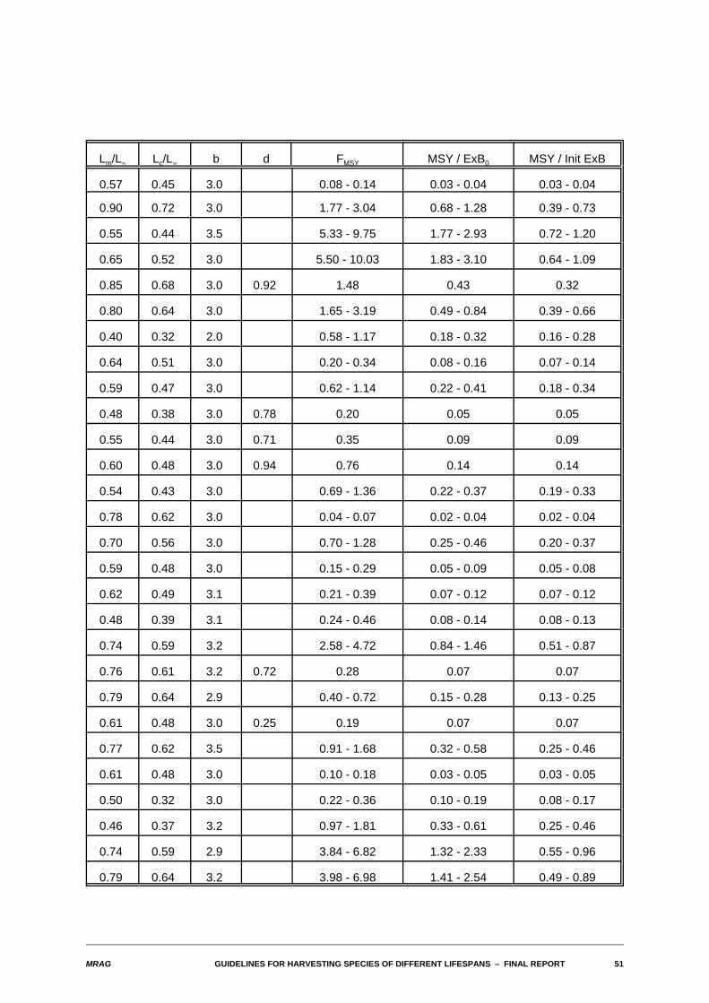
MRAG GUIDELINES FOR HARVESTING SPECIES OF DIFFERENT LIFESPANS S FINAL REPORT 51
Lm/L4 Lc/L4 b d FMSY MSY / ExB0 MSY / Init ExB
0.57 0.45 3.0 0.08 - 0.14 0.03 - 0.04 0.03 - 0.04
0.90 0.72 3.0 1.77 - 3.04 0.68 - 1.28 0.39 - 0.73
0.55 0.44 3.5 5.33 - 9.75 1.77 - 2.93 0.72 - 1.20
0.65 0.52 3.0 5.50 - 10.03 1.83 - 3.10 0.64 - 1.09
0.85 0.68 3.0 0.92 1.48 0.43 0.32
0.80 0.64 3.0 1.65 - 3.19 0.49 - 0.84 0.39 - 0.66
0.40 0.32 2.0 0.58 - 1.17 0.18 - 0.32 0.16 - 0.28
0.64 0.51 3.0 0.20 - 0.34 0.08 - 0.16 0.07 - 0.14
0.59 0.47 3.0 0.62 - 1.14 0.22 - 0.41 0.18 - 0.34
0.48 0.38 3.0 0.78 0.20 0.05 0.05
0.55 0.44 3.0 0.71 0.35 0.09 0.09
0.60 0.48 3.0 0.94 0.76 0.14 0.14
0.54 0.43 3.0 0.69 - 1.36 0.22 - 0.37 0.19 - 0.33
0.78 0.62 3.0 0.04 - 0.07 0.02 - 0.04 0.02 - 0.04
0.70 0.56 3.0 0.70 - 1.28 0.25 - 0.46 0.20 - 0.37
0.59 0.48 3.0 0.15 - 0.29 0.05 - 0.09 0.05 - 0.08
0.62 0.49 3.1 0.21 - 0.39 0.07 - 0.12 0.07 - 0.12
0.48 0.39 3.1 0.24 - 0.46 0.08 - 0.14 0.08 - 0.13
0.74 0.59 3.2 2.58 - 4.72 0.84 - 1.46 0.51 - 0.87
0.76 0.61 3.2 0.72 0.28 0.07 0.07
0.79 0.64 2.9 0.40 - 0.72 0.15 - 0.28 0.13 - 0.25
0.61 0.48 3.0 0.25 0.19 0.07 0.07
0.77 0.62 3.5 0.91 - 1.68 0.32 - 0.58 0.25 - 0.46
0.61 0.48 3.0 0.10 - 0.18 0.03 - 0.05 0.03 - 0.05
0.50 0.32 3.0 0.22 - 0.36 0.10 - 0.19 0.08 - 0.17
0.46 0.37 3.2 0.97 - 1.81 0.33 - 0.61 0.25 - 0.46
0.74 0.59 2.9 3.84 - 6.82 1.32 - 2.33 0.55 - 0.96
0.79 0.64 3.2 3.98 - 6.98 1.41 - 2.54 0.49 - 0.89
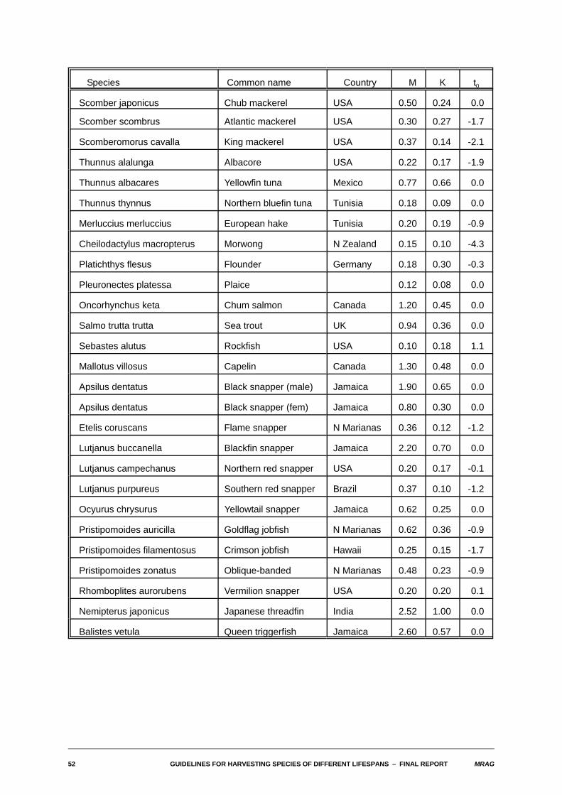
52 GUIDELINES FOR HARVESTING SPECIES OF DIFFERENT LIFESPANS S FINAL REPORT MRAG
Species Common name Country M K t0
Scomber japonicus Chub mackerel USA 0.50 0.24 0.0
Scomber scombrus Atlantic mackerel USA 0.30 0.27 -1.7
Scomberomorus cavalla King mackerel USA 0.37 0.14 -2.1
Thunnus alalunga Albacore USA 0.22 0.17 -1.9
Thunnus albacares Yellowfin tuna Mexico 0.77 0.66 0.0
Thunnus thynnus Northern bluefin tuna Tunisia 0.18 0.09 0.0
Merluccius merluccius European hake Tunisia 0.20 0.19 -0.9
Cheilodactylus macropterus Morwong N Zealand 0.15 0.10 -4.3
Platichthys flesus Flounder Germany 0.18 0.30 -0.3
Pleuronectes platessa Plaice 0.12 0.08 0.0
Oncorhynchus keta Chum salmon Canada 1.20 0.45 0.0
Salmo trutta trutta Sea trout UK 0.94 0.36 0.0
Sebastes alutus Rockfish USA 0.10 0.18 1.1
Mallotus villosus Capelin Canada 1.30 0.48 0.0
Apsilus dentatus Black snapper (male) Jamaica 1.90 0.65 0.0
Apsilus dentatus Black snapper (fem) Jamaica 0.80 0.30 0.0
Etelis coruscans Flame snapper N Marianas 0.36 0.12 -1.2
Lutjanus buccanella Blackfin snapper Jamaica 2.20 0.70 0.0
Lutjanus campechanus Northern red snapper USA 0.20 0.17 -0.1
Lutjanus purpureus Southern red snapper Brazil 0.37 0.10 -1.2
Ocyurus chrysurus Yellowtail snapper Jamaica 0.62 0.25 0.0
Pristipomoides auricilla Goldflag jobfish N Marianas 0.62 0.36 -0.9
Pristipomoides filamentosus Crimson jobfish Hawaii 0.25 0.15 -1.7
Pristipomoides zonatus Oblique-banded N Marianas 0.48 0.23 -0.9
Rhomboplites aurorubens Vermilion snapper USA 0.20 0.20 0.1
Nemipterus japonicus Japanese threadfin India 2.52 1.00 0.0
Balistes vetula Queen triggerfish Jamaica 2.60 0.57 0.0
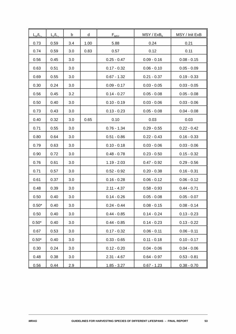
MRAG GUIDELINES FOR HARVESTING SPECIES OF DIFFERENT LIFESPANS S FINAL REPORT 53
Lm/L4 Lc/L4 b d FMSY MSY / ExB0 MSY / Init ExB
0.73 0.59 3.4 1.00 5.88 0.24 0.21
0.74 0.59 3.0 0.83 0.57 0.12 0.11
0.56 0.45 3.0 0.25 - 0.47 0.09 - 0.16 0.08 - 0.15
0.63 0.51 3.0 0.17 - 0.32 0.06 - 0.10 0.05 - 0.09
0.69 0.55 3.0 0.67 - 1.32 0.21 - 0.37 0.19 - 0.33
0.30 0.24 3.0 0.09 - 0.17 0.03 - 0.05 0.03 - 0.05
0.56 0.45 3.2 0.14 - 0.27 0.05 - 0.08 0.05 - 0.08
0.50 0.40 3.0 0.10 - 0.19 0.03 - 0.06 0.03 - 0.06
0.73 0.43 3.0 0.13 - 0.23 0.05 - 0.08 0.04 - 0.08
0.40 0.32 3.0 0.65 0.10 0.03 0.03
0.71 0.55 3.0 0.76 - 1.34 0.29 - 0.55 0.22 - 0.42
0.80 0.64 3.0 0.51 - 0.86 0.22 - 0.43 0.16 - 0.33
0.79 0.63 3.0 0.10 - 0.18 0.03 - 0.06 0.03 - 0.06
0.90 0.72 3.0 0.48 - 0.78 0.23 - 0.50 0.15 - 0.32
0.76 0.61 3.0 1.19 - 2.03 0.47 - 0.92 0.29 - 0.56
0.71 0.57 3.0 0.52 - 0.92 0.20 - 0.38 0.16 - 0.31
0.61 0.37 3.0 0.16 - 0.28 0.06 - 0.12 0.06 - 0.12
0.48 0.39 3.0 2.11 - 4.37 0.58 - 0.93 0.44 - 0.71
0.50 0.40 3.0 0.14 - 0.26 0.05 - 0.08 0.05 - 0.07
0.50* 0.40 3.0 0.24 - 0.44 0.08 - 0.15 0.08 - 0.14
0.50 0.40 3.0 0.44 - 0.85 0.14 - 0.24 0.13 - 0.23
0.50* 0.40 3.0 0.44 - 0.85 0.14 - 0.23 0.13 - 0.22
0.67 0.53 3.0 0.17 - 0.32 0.06 - 0.11 0.06 - 0.11
0.50* 0.40 3.0 0.33 - 0.65 0.11 - 0.18 0.10 - 0.17
0.30 0.24 3.0 0.12 - 0.20 0.04 - 0.06 0.04 - 0.06
0.48 0.38 3.0 2.31 - 4.67 0.64 - 0.97 0.53 - 0.81
0.56 0.44 2.9 1.85 - 3.27 0.67 - 1.23 0.38 - 0.70
54 GUIDELINES FOR HARVESTING SPECIES OF DIFFERENT LIFESPANS S FINAL REPORT MRAG
8. Stochastic recruitment
While deterministic results set a scale on yield levels and indicate how these vary for species with differingbiological parameters, the actual yields that will be taken in the presence of a varying environment candiffer substantially from those suggested by the deterministic results. For many fish species, the primaryfocus of variability is in the annual recruitment; for temperate species the recruitment resulting from thesame or similar levels of spawning stock can vary by more than an order of magnitude. Kirkwood et al(1994) therefore examined the effect of a varying environment by allowing for stochastic variability in thestock-recruitment relationship. The same approach was taken by Beddington and Cooke (1983).
Two scenarios were examined. In the first, the annual recruitment arising from given levels of spawningstock biomass is taken to be log-normally distributed. The second examines the ability of species ofdifferent lifespans to recover from an extreme case of environmental variability, in which the spawningstock suffers an episode of catastrophic mortality.
8.1 Environmental variability in recruitmentIn their examination of the statistical properties of recruitment in some commercial fish species,Hennemuth, Palmer and Brown (1980) found that recruitment was highly variable and that its skewedfrequency distribution was similar to a log-normal distribution. Similar conclusions have been reached inother studies. Accordingly, we investigated the probability distribution of annual yield when the annualrecruitment is log-normally distributed with mean equal to that predicted by the deterministic Beverton-Holtstock-recruitment relationship. The coefficient of variation of the log-normal errors was taken to be 0.5( Beddington and Cooke, 1983).
The procedure for generating series of stochastic annual yields and characterising them for eachcombination of parameters was as follows. A simulated population was set up at time zero in deterministicequilibrium, harvested at the fishing mortality rate that produced the deterministic MSY for that parametercombination. Annual log normal variation about the stock-recruitment curve was then introduced, andsufficient time was allowed to elapse for the effects of the stochastic recruitment to spread through all ageclasses in the population. Then the values of annual yield were collected for the next 100 years. Thisprocess was repeated 100 times, and the median, 5th and 95th percentiles of the pooled distribution ofannual yields was determined. These statistics of the distribution of annual yield were determined inKirkwood et al (1994) for parameter combinations lc=0.4, lm=0.5, d=0.2 and 0.8, and M taking selectedvalues in the range 0.05 to 3.0. Results were presented in terms of the ratios of annual yield to thedeterministic exploitable biomass.
For low values of M, the median annual yield exploitable biomass ratio was very close to thecorresponding deterministic value, but as M increased, the median began to fall below the deterministicvalue. This tendency is more marked when the degree of density dependence in the stock-recruitmentrelationship was much smaller (d=0.2).
There was a strong tendency for increased skewness in the distribution of annual yield biomass ratios asM increased. The lower 5th percentile of this distribution stayed remarkably constant for M above 0.5, butin contrast the 95th percentile increased rapidly with M. The increasing skewness with increasing M wasexpected; when M is high, the exploitable stock consists of only one or two age classes, each of whichhas been subject to highly skewed log-normal variability, while when M is low, the exploitable stock is thesum of many age classes and its distribution will be more symmetric.
A direct result of the increasing skewness with M is that, while in most cases the annual yield biomassratio will be much less than ½M, in an important minority of cases it can exceed ½M, sometimessubstantially. This ability to gain benefits in terms of high yields during good years flows directly from theassumption that fishing mortality (or equivalently fishing effort) is the variable that is used to control thelevel of harvesting. The figures in Kirkwood et al (1994) show clearly that once M gets large, applicationof a constant fishing mortality can lead to yield-biomass ratios considerably in excess of ½M. However,the very high variation in recruitment has tended to be documented for species with relatively low mortality.
8.2 Recovery from a stock collapseThe preceding sub-section examined the effect of stochastic variation of recruitment about a stock-recruitment relationship. One feature of that relationship was that recruitment was non-zero for all positivestock biomasses. This would be an optimistic assumption if there existed a critical spawning stockbiomass below which recruitment fell to zero; i.e. if there is critical depensation in the stock-recruitment
MRAG GUIDELINES FOR HARVESTING SPECIES OF DIFFERENT LIFESPANS S FINAL REPORT 55
relationship. Here, Kirkwood et al (1994) examined the ability of a population to recover from acatastrophic mortality episode.
A population was assumed to be in deterministic equilibrium at time zero, and harvested at the fishingmortality rate that produces the deterministic MSY. Just before the start of the spawning season in the firstyear, the entire spawning stock was killed, so that there was no recruitment at all at the beginning of thesecond year. Subsequently, the population was allowed to recover, if it can, according to the standarddeterministic dynamics and deterministic stock-recruitment relationship. During the recovery period, fishingcontinued at the FMSY rate.
The trajectories taken by the annual spawning stock biomasses were investigated for three differentnatural mortality rates (M = 0.05, 0.1 and 0.4). For convenience,the lengths at first capture and at maturitywere taken to be equal. A low degree of density dependence in the stock recruitment relationship wasused (d=0.2), and M/K was set to 1.0. The resulting trajectories are shown in Kirkwood et al (1994).
Despite exploitation continuing, in each case the spawning stock biomasses recovered (eventually),initially at a relatively fast rate and then at a rather slower rate. The key to these recoveries lay in thepresence of a buffer in the form of unfished immature age-classes in the population, and in the time lagsbetween birth and the age at maturity. For each of the three mortality rates, the age at maturity was morethan one year, so that immediately after the catastrophic mortality suffered by the spawning stock, thepopulation consisted of a number of immature unfished age-classes. The number of such age-classesincreased with decreasing values of M. One year later, the oldest of these immature age-classes becamemature and the process of rebuilding the spawning stock started. This process continued until the annualincrement to the spawning stock was roughly balanced by the deaths due to natural mortality and fishing.The spawning stock then recovered at a much slower rate that is consistent with the increase inrecruitment flowing from an increased spawning stock implied by the stock-recruitment relationship .
The exclusion of examples with a high M is deliberate. Under the conditions simulated, any species withM sufficiently high that the age at maturity is less than one year will by definition be completelyextinguished by the catastrophe hypothesised. This may seem an artifact of an extremely unlikelyscenario. While in a strict sense that is true, all that is required to bring about conditions nearly matchingthose simulated here for short-lived species is for them to have a critical spawning biomass below whichrecruitment is severely diminished. Then a bout of severe overfishing, for example, could well result in acomplete stock collapse.
In contrast, the unfished age-classes in longer-lived species provide a buffer against such catastrophicevents. It follows that in this sense, longer-lived species can show a greater resilience than short-livedones. Further, the greater the number of unfished age-classes, the greater the amount of buffering. Thusextremely long-lived fish species, such as orange roughy, have the ability to withstand occasional majorcatastrophic events, despite the very low sustainable yields they provide.
56 GUIDELINES FOR HARVESTING SPECIES OF DIFFERENT LIFESPANS S FINAL REPORT MRAG
9. Conclusions
The primary conclusion that may be drawn from the results obtained during the project is that althoughthere is a clear approximately proportional relationship between sustainable yield and mortality (lifespan),the constant of proportionality is smaller than had originally been proposed by Gulland (1971). Yield takenas a percentage of virgin biomass, even in the case of very strong density dependence (recruitmentconstant regardless of mature stock size), is more likely to be around 0.3M, rather than 0.5M that Gullandsuggested. When more realistic levels of density dependence are considered, the percentage yield isfurther reduced, perhaps to between 0.1M and 0.2M.
When looked at specifically in terms of lifespans, the non-linear relationship between M and lifespanimplies that for longer-lived species, the sustainable yields are both low and almost independent oflifespan. An exception to this ground rule is the behaviour of very short lived species. In these, the detailsof the life cycle dominate their response to exploitation, such that on sensible and measurable definitionsof exploitable biomass, the stock may be capable of producing sustainable yields well in excess of thebiomass measured at the start of the fishing season.
Obviously, this analysis sets the scene for more detailed investigations of individual species and the wayin which the key parameters that determine yields vary. An initial step has been taken using theinformation recorded in the FISHBASE database to develop the estimates of yield-biomass ratios andfishing mortality rates for selected species given in section 7 of this summary report. In a more generalcontext, it is interesting to note that Pauly (1980) found a dependence between natural mortality, growthin size, and mean water temperature for a wide range of fish stocks. Such a relationship affords thepossibility of further assessment of the potential yield of species in ecosystems of different types.
The deterministic results are a useful guide to expectations in the real world, particularly for relatively longlived species. The investigation of stochasticity in recruitment and its implications for the expectedvariation in yield complements other findings that a policy of constant effort with a target level of fishingmortality can produce substantial benefits in high yields when recruitment is high. The strength of thiseffect with increasing mortality (reduced lifespan) is particularly marked. Very short lived species doappear to be exceptions to the general rules outlined above; they can provide high yields. However thebrief examination of the effect of catastrophic events on the dynamics does indicate that longer livedspecies retain a resilience to catastrophes that is not available to the short lived species, which can beparticularly vulnerable to a combination of high exploitation and occasional environmental events thatdevastate the spawning stock.
MRAG GUIDELINES FOR HARVESTING SPECIES OF DIFFERENT LIFESPANS S FINAL REPORT 57
10. References
Beddington, J.R. & Basson, M. (1994) The limits to exploitation on land and sea. PhilosophicalTransactions of the Royal Society London Series B. 343: 87-92.
Beddington, J.R. & Cooke, J.G. (1983) The potential yield of fish stocks. FAO Fisheries Technical Paper242.
Beddington, J.R. & May, R.M. (1977) Harvesting natural populations in a randomly fluctuatingenvironment. Science, 197, 463-465.
Beddington, J.R., Rosenberg, A.A., Crombie, J.A. & Kirkwood, G.P. (1990) Stock assessment and theprovision of management advice for the short fin squid fishery in Falkland Islands waters. FisheriesResearch 8, 351-365.
Beverton, R.J.H. & Holt, S.J. (1957) On the dynamics of exploited fish populations. MAFF FisheriesInvestigations London, Series 2, 19, 1-533.
von Bertalanffy, L. (1938) A quantitative theory of organic growth. Human Biology, 10, 181-213.
Gulland, J.A. (1971) The fish resources of the ocean. Fishing News Books Ltd., West Byfleet, Surrey.
Heincke, F. (1913) Investigations on the plaice. General report. 1. The plaice fishery and protectivemeasures. Preliminary brief summary of the most important points of the report. ConseilInternational pour l'Exploration de la Mer, Rapports et Procés-Verbaux des Réunions 16, 1-67.
Hennemuth, R.C., Palmer, J.E. & Brown, B.E. (1980) A statistical description of recruitment in eighteenselected fish stocks. Journal of Northwest Atlantic Fisheries Science, 1, 101-111.
Kirkwood, G.P., Beddington, J.R. & J.A. Rossouw. (1994) Harvesting species of different lifespans. pp199-227 in Edwards, P.J., May, R. and Webb, N.R. (Eds) "Large Scale Ecology and ConservationBiology". Blackwell Scientific Publications.
Mace, P.M. & Sissenwine, M.P. (1993) How much spawning per recruit is enough? In Smith, S.J., Hunt,J.J. and Rivard, D. (Eds.) Risk evaluation and biological reference points for fisheries management.Canadian Special Publication on Fisheries and Aquatic Science 120: 101-118.
Mace, P.M. (1994) Relationships between common biological reference points used as thresholds andtargets of fishery management strategies. Canadian Journal of Fisheries and Aquatic Science51:110-122.
Myers, R.R., Rosenberg, A.A., Mace, P., Barrowman, N. & Restrepo, V. (1994) In search of thresholdsfor recruitment overfishing.
Pauly, D. (1980) On the interrelationships between natural mortality, growth parameters, and meanenvironmental temperature in 175 fish stocks. Journal du Conseil International pour l'Explorationde la Mer, 11, 559-623.
Pauly, D. & Soriano, M.L. (1986) Some practical extensions to Beverton and Holt's relative yield-per-recruit model, p. 491-495. In Maclean, J.L., Dizon, L.B. & Hosillos, L.V. (Eds.) The First AsianFisheries Forum. Asian Fisheries Society, Manila, Philippines.
Ricker, W.E. (1954) Stock and recruitment. Journal of the Fisheries Research Board of Canada 30, 1965-1976.
Shepherd, J.G. (1982) A family of general production curves for exploited populations. MathematicalBiosciences, 59, 77-93.