how will longer lifespans affect state and local …

R E S E A R C HRETIREMENT

State and Local Pension Plans Number 43, April 2015

HOW WILL LONGER LIFESPANS AFFECT STATE AND LOCAL PENSION FUNDING?

By Alicia H. Munnell, Jean-Pierre Aubry, and Mark Cafarelli*

* Alicia H. Munnell is director of the Center for Retirement Research at Boston College (CRR) and the Peter F. Drucker Professor of Management Sciences at Boston College’s Carroll School of Management. Jean-Pierre Aubry is assistant director of state and local research at the CRR. Mark Cafarelli is a re-search associate at the CRR. The authors wish to thank David Blitzstein, Keith Brainard, Gene Kalwarski and his colleagues at Cheiron, Steven Kreisberg, and Joseph Silvestri for helpful comments.

Introduction

The fact that people are living longer is good news from a human perspective. But longer lifespans also make defined benefit pension plans more expensive because sponsors must pay benefits to retirees for a longer period of time. The question is the extent to which state and local plans have already incorporated this pattern of continued longevity improvement into their cost estimates. For example, CalPERS – one of the nation’s largest plans – revised its longevity assumptions in 2014, significantly increasing its liabilities and reducing its funded ratio by 5 percent-age points. This change raises the question whether more cost increases due to longevity improvements are on the horizon. To answer the question, this brief explores what public plan liabilities and funded ratios would look like under two alternative scenarios: 1) if public plans were required to use the new mortality table designed for private sector plans; and 2) if public plans were required to go one step further and fully incorporate expected future mortality improvements.

The discussion proceeds as follows. The first section describes how public and private plans cur-rently incorporate longevity improvements into their cost estimates. The second section presents a simple model that relates the impact of improved longev-ity to liabilities, showing that, if beneficiaries live an additional year, liabilities increase by 3.5 percent. The third section estimates the impact of changing the longevity assumptions to: 1) the new standard designed for use in the private sector; and 2) the more stringent standard that incorporates future mortality improvements. The results suggest that, under the first standard, public plans underestimate life expec-tancy by only 0.5 year. Adopting the second standard would increase life expectancy by 2.3 years and reduce the funded ratio of public plans from 73 percent to 67 percent. Of course, public plans vary significantly, so the impacts would be much larger for some and smaller for others.

LEARN MORE

Search for other publications on this topic at:crr.bc.edu

Center for Retirement Research2

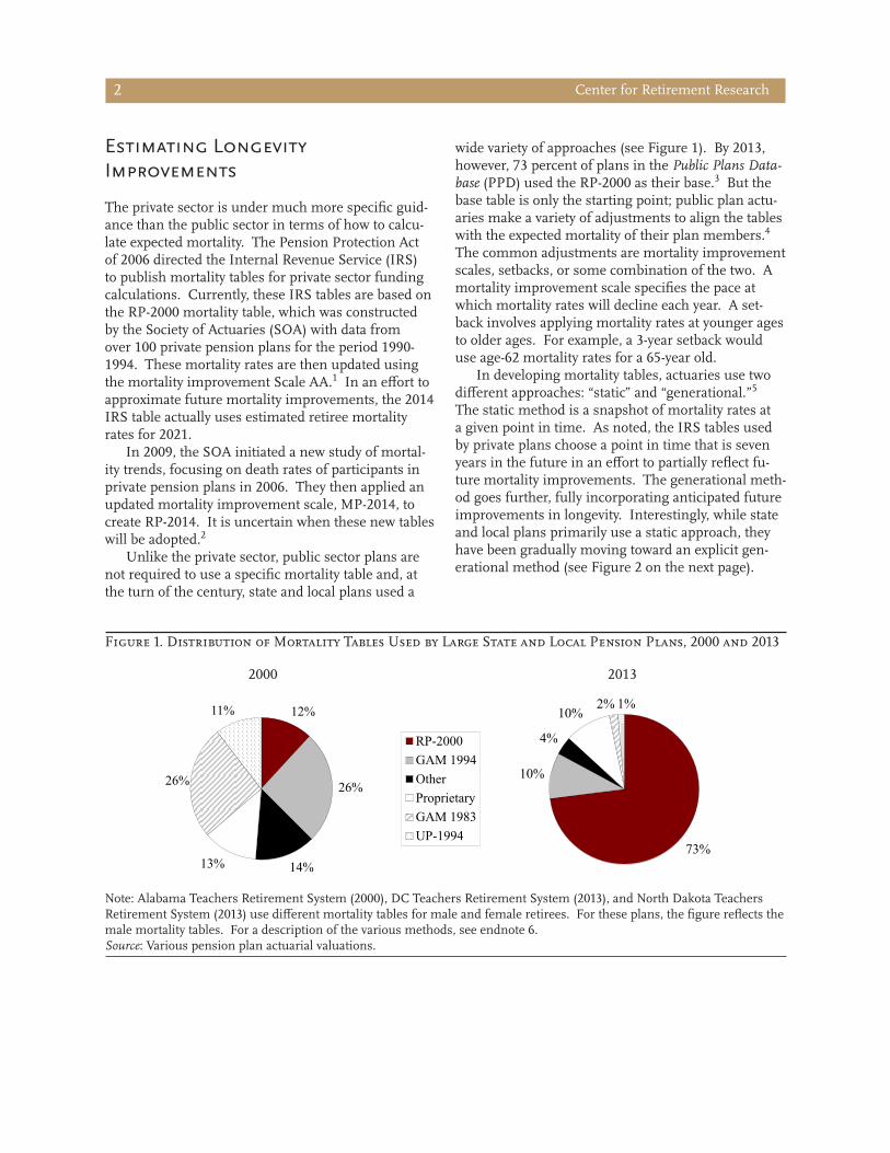
Note: Alabama Teachers Retirement System (2000), DC Teachers Retirement System (2013), and North Dakota Teachers Retirement System (2013) use different mortality tables for male and female retirees. For these plans, the figure reflects the male mortality tables. For a description of the various methods, see endnote 6. Source: Various pension plan actuarial valuations.

Estimating Longevity Improvements

The private sector is under much more specific guid-ance than the public sector in terms of how to calcu-late expected mortality. The Pension Protection Act of 2006 directed the Internal Revenue Service (IRS) to publish mortality tables for private sector funding calculations. Currently, these IRS tables are based on the RP-2000 mortality table, which was constructed by the Society of Actuaries (SOA) with data from over 100 private pension plans for the period 1990-1994. These mortality rates are then updated using the mortality improvement Scale AA.1 In an effort to approximate future mortality improvements, the 2014 IRS table actually uses estimated retiree mortality rates for 2021.

In 2009, the SOA initiated a new study of mortal-ity trends, focusing on death rates of participants in private pension plans in 2006. They then applied an updated mortality improvement scale, MP-2014, to create RP-2014. It is uncertain when these new tables will be adopted.2

Unlike the private sector, public sector plans are not required to use a specific mortality table and, at the turn of the century, state and local plans used a

Figure 1. Distribution of Mortality Tables Used by Large State and Local Pension Plans, 2000 and 2013

wide variety of approaches (see Figure 1). By 2013, however, 73 percent of plans in the Public Plans Data-base (PPD) used the RP-2000 as their base.3 But the base table is only the starting point; public plan actu-aries make a variety of adjustments to align the tables with the expected mortality of their plan members.4 The common adjustments are mortality improvement scales, setbacks, or some combination of the two. A mortality improvement scale specifies the pace at which mortality rates will decline each year. A set-back involves applying mortality rates at younger ages to older ages. For example, a 3-year setback would use age-62 mortality rates for a 65-year old.

In developing mortality tables, actuaries use two different approaches: “static” and “generational.”5 The static method is a snapshot of mortality rates at a given point in time. As noted, the IRS tables used by private plans choose a point in time that is seven years in the future in an effort to partially reflect fu-ture mortality improvements. The generational meth-od goes further, fully incorporating anticipated future improvements in longevity. Interestingly, while state and local plans primarily use a static approach, they have been gradually moving toward an explicit gen-erational method (see Figure 2 on the next page).

2000 2013

12%

26%

14%13%

26%

11%

RP-2000GAM 1994OtherProprietaryGAM 1983UP-1994

73%

10%

4%

10%2% 1%

Issue in Brief 3

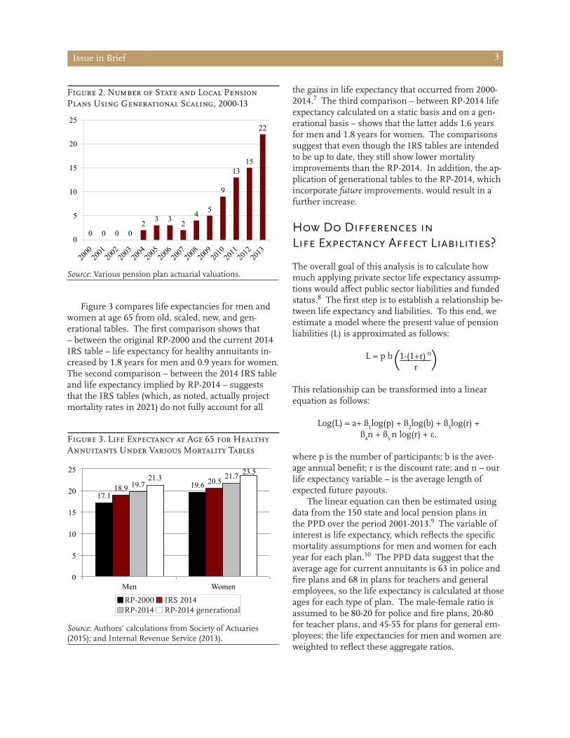
Figure 3 compares life expectancies for men and women at age 65 from old, scaled, new, and gen-erational tables. The first comparison shows that – between the original RP-2000 and the current 2014 IRS table – life expectancy for healthy annuitants in-creased by 1.8 years for men and 0.9 years for women. The second comparison – between the 2014 IRS table and life expectancy implied by RP-2014 – suggests that the IRS tables (which, as noted, actually project mortality rates in 2021) do not fully account for all

the gains in life expectancy that occurred from 2000-2014.7 The third comparison – between RP-2014 life expectancy calculated on a static basis and on a gen-erational basis – shows that the latter adds 1.6 years for men and 1.8 years for women. The comparisons suggest that even though the IRS tables are intended to be up to date, they still show lower mortality improvements than the RP-2014. In addition, the ap-plication of generational tables to the RP-2014, which incorporate future improvements, would result in a further increase.

How Do Differences in Life Expectancy Affect Liabilities?

The overall goal of this analysis is to calculate how much applying private sector life expectancy assump-tions would affect public sector liabilities and funded status.8 The first step is to establish a relationship be-tween life expectancy and liabilities. To this end, we estimate a model where the present value of pension liabilities (L) is approximated as follows:

L = p b 1-(1+r)-n

r

This relationship can be transformed into a linear equation as follows:

Log(L) = a+ ß1log(p) + ß

2log(b) + ß

3log(r) +

ß4n + ß

5 n log(r) + ε,

where p is the number of participants; b is the aver-age annual benefit; r is the discount rate; and n – our life expectancy variable – is the average length of expected future payouts.

The linear equation can then be estimated using data from the 150 state and local pension plans in the PPD over the period 2001-2013.9 The variable of interest is life expectancy, which reflects the specific mortality assumptions for men and women for each year for each plan.10 The PPD data suggest that the average age for current annuitants is 63 in police and fire plans and 68 in plans for teachers and general employees, so the life expectancy is calculated at those ages for each type of plan. The male-female ratio is assumed to be 80-20 for police and fire plans, 20-80 for teacher plans, and 45-55 for plans for general em-ployees; the life expectancies for men and women are weighted to reflect these aggregate ratios.

Source: Various pension plan actuarial valuations.

Figure 2. Number of State and Local Pension Plans Using Generational Scaling, 2000-13

Source: Authors’ calculations from Society of Actuaries (2015); and Internal Revenue Service (2013).

Figure 3. Life Expectancy at Age 65 for Healthy Annuitants Under Various Mortality Tables

0 0 0 02 3 3 2

4 5

9

1315

22

0

5

10

15

20

25

17.1 19.6 18.9

20.5 19.7 21.7 21.3

23.5

0

5

10

15

20

25

Men Women

RP-2000 IRS 2014 RP-2014 RP-2014 generational

( )


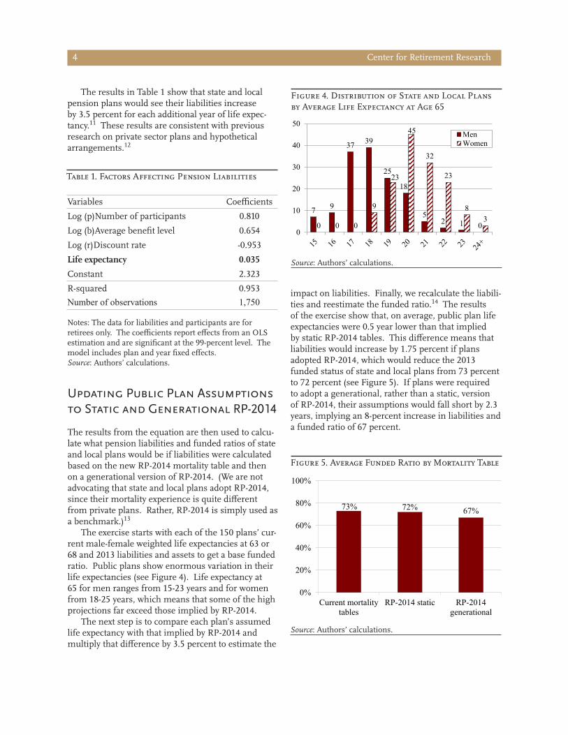
The results in Table 1 show that state and local pension plans would see their liabilities increase by 3.5 percent for each additional year of life expec-tancy.11 These results are consistent with previous research on private sector plans and hypothetical arrangements.12

impact on liabilities. Finally, we recalculate the liabili-ties and reestimate the funded ratio.14 The results of the exercise show that, on average, public plan life expectancies were 0.5 year lower than that implied by static RP-2014 tables. This difference means that liabilities would increase by 1.75 percent if plans adopted RP-2014, which would reduce the 2013 funded status of state and local plans from 73 percent to 72 percent (see Figure 5). If plans were required to adopt a generational, rather than a static, version of RP-2014, their assumptions would fall short by 2.3 years, implying an 8-percent increase in liabilities and a funded ratio of 67 percent.

Notes: The data for liabilities and participants are for retirees only. The coefficients report effects from an OLS estimation and are significant at the 99-percent level. The model includes plan and year fixed effects.Source: Authors’ calculations.

Table 1. Factors Affecting Pension Liabilities

Variables Coefficients

Log (p)Number of participants 0.810

Log (b)Average benefit level 0.654

Log (r)Discount rate -0.953

Life expectancy 0.035

Constant 2.323

R-squared 0.953

Number of observations 1,750

Updating Public Plan Assumptions to Static and Generational RP-2014

The results from the equation are then used to calcu-late what pension liabilities and funded ratios of state and local plans would be if liabilities were calculated based on the new RP-2014 mortality table and then on a generational version of RP-2014. (We are not advocating that state and local plans adopt RP-2014, since their mortality experience is quite different from private plans. Rather, RP-2014 is simply used as a benchmark.)13

The exercise starts with each of the 150 plans’ cur-rent male-female weighted life expectancies at 63 or 68 and 2013 liabilities and assets to get a base funded ratio. Public plans show enormous variation in their life expectancies (see Figure 4). Life expectancy at 65 for men ranges from 15-23 years and for women from 18-25 years, which means that some of the high projections far exceed those implied by RP-2014.

The next step is to compare each plan’s assumed life expectancy with that implied by RP-2014 and multiply that difference by 3.5 percent to estimate the

Source: Authors’ calculations.

Figure 4. Distribution of State and Local Plans by Average Life Expectancy at Age 65


Figure 5. Average Funded Ratio by Mortality Table

7 9

37 39

25

18

52 1 00 0 0

9

23

45

32

23

83

0

10

20

30

40

50MenWomen

73% 72% 67%

0%

20%

40%

60%

80%

100%

Current mortalitytables

RP-2014 static RP-2014generational

Issue in Brief 5

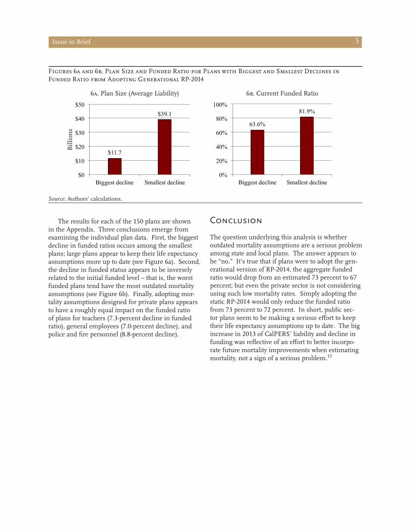
The results for each of the 150 plans are shown in the Appendix. Three conclusions emerge from examining the individual plan data. First, the biggest decline in funded ratios occurs among the smallest plans; large plans appear to keep their life expectancy assumptions more up to date (see Figure 6a). Second, the decline in funded status appears to be inversely related to the initial funded level – that is, the worst funded plans tend have the most outdated mortality assumptions (see Figure 6b). Finally, adopting mor-tality assumptions designed for private plans appears to have a roughly equal impact on the funded ratio of plans for teachers (7.3-percent decline in funded ratio), general employees (7.0-percent decline), and police and fire personnel (8.8-percent decline).

Conclusion

The question underlying this analysis is whether outdated mortality assumptions are a serious problem among state and local plans. The answer appears to be “no.” It’s true that if plans were to adopt the gen-erational version of RP-2014, the aggregate funded ratio would drop from an estimated 73 percent to 67 percent; but even the private sector is not considering using such low mortality rates. Simply adopting the static RP-2014 would only reduce the funded ratio from 73 percent to 72 percent. In short, public sec-tor plans seem to be making a serious effort to keep their life expectancy assumptions up to date. The big increase in 2013 of CalPERS’ liability and decline in funding was reflective of an effort to better incorpo-rate future mortality improvements when estimating mortality, not a sign of a serious problem.15


Figures 6a and 6b. Plan Size and Funded Ratio for Plans with Biggest and Smallest Declines in Funded Ratio from Adopting Generational RP-2014

6a. Plan Size (Average Liability) 6b. Current Funded Ratio

$11.7

$39.1

$0

$10

$20

$30

$40

$50

Biggest decline Smallest decline

63.6%

81.9%

0%

20%

40%

60%

80%

100%

Biggest decline Smallest decline

Bill

ion

s


1 For example, the mortality rate for a 65-year-old man in the RP-2000 is 1.3 percent and the annual per-centage decline in mortality based on the Scale AA is 1.4 percent, so to calculate the mortality rate in 2014 requires reducing the initial rate by 1.4 percent for 14 years – producing a 2014 mortality rate of 1.1 percent. 2 Some critics suggest that, because of the sample used, RP-2014 may be biased toward faster rates of longevity improvement. See American Academy of Actuaries Pension Committee (2014).

3 The PPD is developed and maintained through a collaboration of the Center for Retirement Research at Boston College, the Center for State and Local Government Excellence, and the National Associa-tion of State Retirement Administrators. It contains data for 150 large state and local plans – 114 state and 36 local – and accounts for 91 percent of assets and workers relative to the totals reported by the U.S. Census Bureau.

4 Plan actuaries perform periodic experience stud-ies (every three to five years for most large plans) to ensure that assumptions used by the plan align with the plan’s actual mortality experience.

5 Alternative terms for “static” and “generational” projections of life expectancy are, respectively, “pe-riod” and “cohort.” An example of how the two ap-proaches differ may be helpful. Under the basic static method, for a 65-year-old in 2015 the mortality rates at 66, 67, 68 etc. are the rates applicable to individuals currently at those ages in 2015. In contrast, a “genera-tional” approach would take into account that mortal-ity rates for individuals would likely decline in the future. Thus, for a 65-year-old in 2015, the mortality rate at 66 would be that for a 66-year-old in 2016; at 67 that for a 67-year-old in 2017, etc. Since death rates are projected to decline in the future, a static calcula-tion significantly understates how long someone is actually likely to live. 6 Each mortality table is based on different sources of actual mortality experience. The RP-2000 is described in the text. The UP-1994 (Uninsured Pensioner) tables are based on group annuitant experience from 1985-1990, the federal Civil Service Retirement Sys-tem experience, and Social Security’s Actuarial Study No. 107. The 1994 GAM (Group Annuity Mortality)

tables are based on the same experience as UP-94 except that the GAM-94 tables include a 7-percent margin designed for insurance reserves. The 1983 GAM tables are based on insured group annuity ex-perience submitted by Prudential and by the Bankers Life, U.S. white population statistics for the period from 1965-1978, Canadian population statistics from 1966-1976, and mortality rates for persons covered under Medicare during 1973-1977.

7 To test for consistency between the RP-2014 and the RP-2000 rates, SOA actuaries applied both the Scale AA and the Scale MP-2014 to the RP-2000 rates and concluded that the Scale MP-2014 was more ac-curate.

8 The following analysis builds on a similar study by Kisser et al. (2012) for private defined benefit plans over the period 1995-2007.

9 Complete historical data are not available for every plan, so the total number of observations is 1,750.

10 Life expectancy can be derived from mortality rates in three steps: 1) compute survival rates from mortality rates – that is, a 1-percent chance of dy-ing turns into a 99-percent chance of surviving; 2) calculate the probability of, say, a 65-year-old living to 66, to 67, to 68 and so on, where each year’s rate is the product of the previous survival rates; and 3) sum the conditional survival rates to determine the number of years the 65-year-old is expected to live.

11 The dependent variable is the liability for annui-tants – that is, for those already retired. The percent-age increase in active worker liability will be of a similar order of magnitude.

12 Antolin (2007) computes pension liabilities for a hypothetical pension fund that is closed to new en-trants and finds that an unexpected improvement in life expectancy of one year per decade could increase pension liabilities by 8-10 percent. Dushi, Friedberg, and Webb (2010) find that updating the mortality tables used to estimate the pension liabilities reported on Forms 10-K, which typically reflect mortality rates in the early 1980s, would increase life expectancy at age 60 by about three years and increase liabilities by 12 percent for the average male plan participant. Kisser et al. (2012) estimate the above equation for

Endnotes

Issue in Brief 7

References

American Academy of Actuaries Pension Committee. 2014. RP-2014 and MP-2014 Comments. Washing-ton, DC.

Antolin, Pablo. 2007. “Longevity Risk and Private Pen-sions.” OECD Working Papers on Insurance and Private Pensions 3:1-28. Paris, France.

CalPERS Actuarial Office. 2014. CalPERS Experience Study and Review of Actuarial Assumptions. Sacra-mento, CA.

Dushi, Irena, Leora Friedberg, and Anthony Webb. 2010. “The Impact of Aggregate Mortality Risk on Defined Benefit Pension Plans.” Journal of Pension Economics and Finance 9: 481-503.

Internal Revenue Service. 2013. Updated Static Mor-tality Tables for the Years 2014 and 2015. Notice 2013-49. Washington, DC.

Kisser, Michael, John Kiff, Eric Oppers, and Mauricio Soto. 2012. “The Impact of Longevity Improve-ments on U.S. Corporate Defined Benefit Plans.” Working Paper. Washington, DC: International Monetary Fund.

Public Plans Database. 2001-2013. Center for Retire-ment Research at Boston College, Center for State and Local Government Excellence, and National Association of State Retirement Administrators.

Society of Actuaries. 2015. Mortality and Other Rate Tables. Chicago, IL. Database available at http://mort.soa.org/

private defined benefit plans and find that an addi-tional year of life expectancy increases liabilities by about 3 percent.

13 Public plans were excluded from the mortality data used to create RP-2014 because their mortality experience differed significantly from those of private plans for which the RP-2014 table was devised. In response to comments, the SOA recommended a separate study of public plan mortality experience, with the expectation that the study would include separate tables for public safety workers, teachers, and other public entities.

14 The variation in assumptions and methodology means that some rules are required to determine how plans would respond to the imposition of RP-2014. First – for plans that currently use the static method – if a plan’s current life expectancy exceeds that implied by RP-2014, we assume that the plan maintains its current life expectancy under the RP-2014 static sce-nario. In these cases, to project life expectancy under the generational approach, we add the difference between the RP-2014 static and generational assump-tions to the plan’s own static assumption. Second – for plans that currently use the generational method – we calculate a new life expectancy only under the RP-2014 generational scenario and do not include any estimate of life expectancy under the RP-2014 static scenario.

15 Specifically, CalPERS shifted from virtually no projection of future mortality improvement to a 20-year static projection (the approximate duration of CalPERS’ benefit payments).

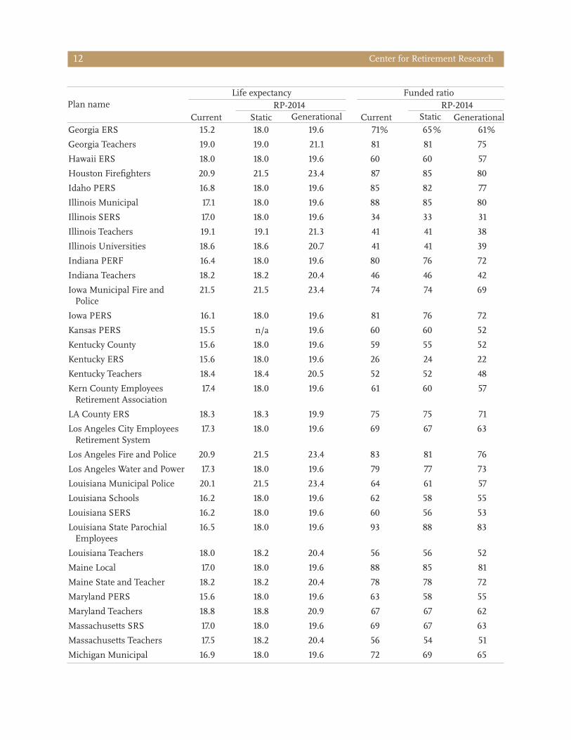
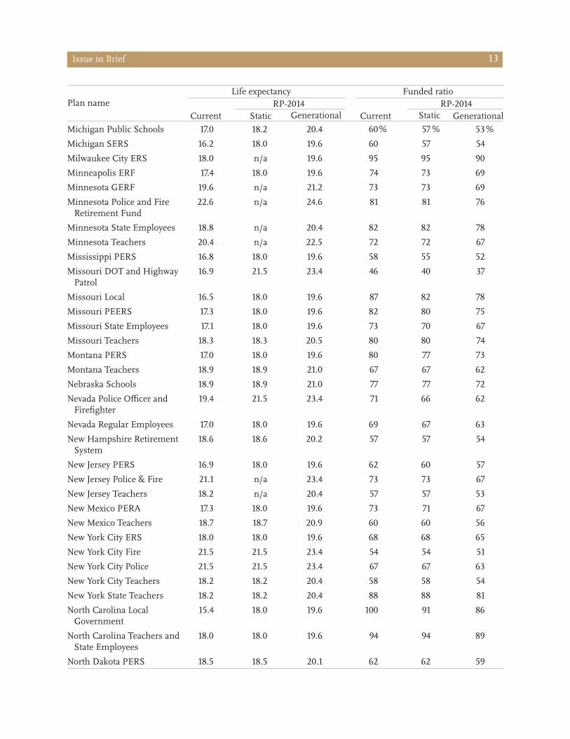
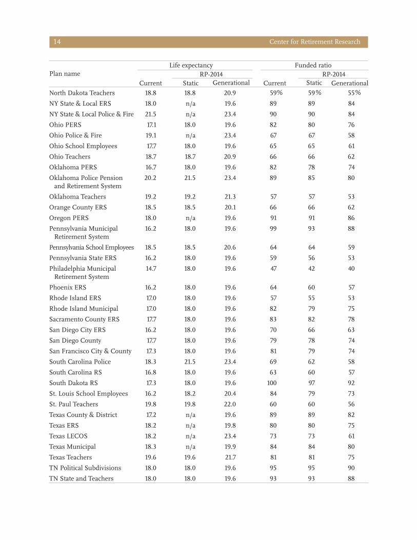
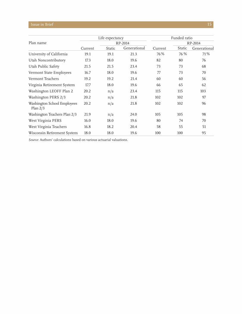
APPENDIX

Issue in Brief 9

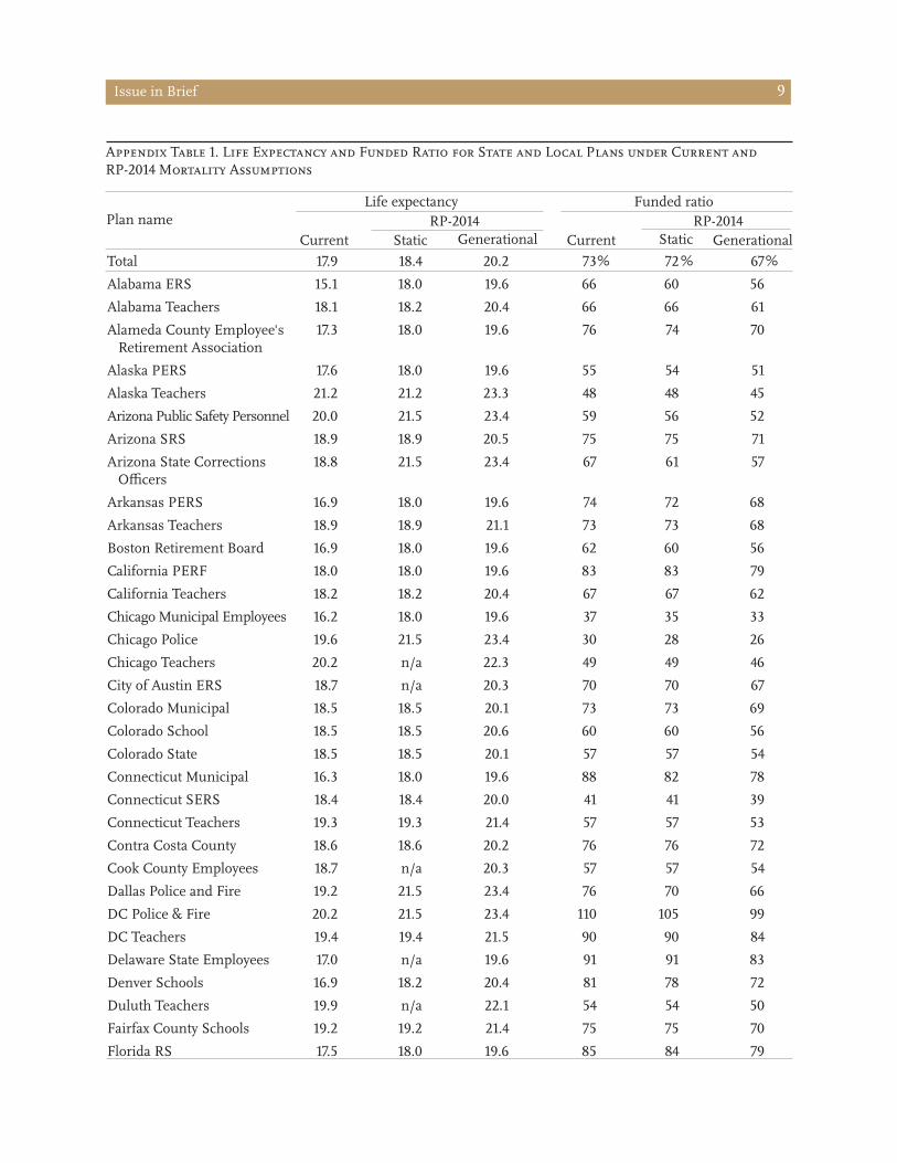
Total 17.9 18.4 20.2 73 72 67

Alabama ERS 15.1 18.0 19.6 66 60 56

Alabama Teachers 18.1 18.2 20.4 66 66 61

Alameda County Employee's Retirement Association

17.3 18.0 19.6 76 74 70

Alaska PERS 17.6 18.0 19.6 55 54 51

Alaska Teachers 21.2 21.2 23.3 48 48 45

Arizona Public Safety Personnel 20.0 21.5 23.4 59 56 52

Arizona SRS 18.9 18.9 20.5 75 75 71

Arizona State Corrections Officers

18.8 21.5 23.4 67 61 57

Arkansas PERS 16.9 18.0 19.6 74 72 68

Arkansas Teachers 18.9 18.9 21.1 73 73 68

Boston Retirement Board 16.9 18.0 19.6 62 60 56

California PERF 18.0 18.0 19.6 83 83 79

California Teachers 18.2 18.2 20.4 67 67 62

Chicago Municipal Employees 16.2 18.0 19.6 37 35 33

Chicago Police 19.6 21.5 23.4 30 28 26

Chicago Teachers 20.2 n/a 22.3 49 49 46

City of Austin ERS 18.7 n/a 20.3 70 70 67

Colorado Municipal 18.5 18.5 20.1 73 73 69

Colorado School 18.5 18.5 20.6 60 60 56

Colorado State 18.5 18.5 20.1 57 57 54

Connecticut Municipal 16.3 18.0 19.6 88 82 78

Connecticut SERS 18.4 18.4 20.0 41 41 39

Connecticut Teachers 19.3 19.3 21.4 57 57 53

Contra Costa County 18.6 18.6 20.2 76 76 72

Cook County Employees 18.7 n/a 20.3 57 57 54

Dallas Police and Fire 19.2 21.5 23.4 76 70 66

DC Police & Fire 20.2 21.5 23.4 110 105 99

DC Teachers 19.4 19.4 21.5 90 90 84

Delaware State Employees 17.0 n/a 19.6 91 91 83

Denver Schools 16.9 18.2 20.4 81 78 72

Duluth Teachers 19.9 n/a 22.1 54 54 50

Fairfax County Schools 19.2 19.2 21.4 75 75 70

Florida RS 17.5 18.0 19.6 85 84 79

Appendix Table 1. Life Expectancy and Funded Ratio for State and Local Plans under Current and RP-2014 Mortality Assumptions

Plan nameLife expectancy Funded ratio

RP-2014 RP-2014Current CurrentStatic StaticGenerational Generational

% % %

Georgia ERS 15.2 18.0 19.6 71 65 61

Georgia Teachers 19.0 19.0 21.1 81 81 75

Hawaii ERS 18.0 18.0 19.6 60 60 57

Houston Firefighters 20.9 21.5 23.4 87 85 80

Idaho PERS 16.8 18.0 19.6 85 82 77

Illinois Municipal 17.1 18.0 19.6 88 85 80

Illinois SERS 17.0 18.0 19.6 34 33 31

Illinois Teachers 19.1 19.1 21.3 41 41 38

Illinois Universities 18.6 18.6 20.7 41 41 39

Indiana PERF 16.4 18.0 19.6 80 76 72

Indiana Teachers 18.2 18.2 20.4 46 46 42

Iowa Municipal Fire and Police

21.5 21.5 23.4 74 74 69

Iowa PERS 16.1 18.0 19.6 81 76 72

Kansas PERS 15.5 n/a 19.6 60 60 52

Kentucky County 15.6 18.0 19.6 59 55 52

Kentucky ERS 15.6 18.0 19.6 26 24 22

Kentucky Teachers 18.4 18.4 20.5 52 52 48

Kern County Employees Retirement Association

17.4 18.0 19.6 61 60 57

LA County ERS 18.3 18.3 19.9 75 75 71

Los Angeles City Employees Retirement System

17.3 18.0 19.6 69 67 63

Los Angeles Fire and Police 20.9 21.5 23.4 83 81 76

Los Angeles Water and Power 17.3 18.0 19.6 79 77 73

Louisiana Municipal Police 20.1 21.5 23.4 64 61 57

Louisiana Schools 16.2 18.0 19.6 62 58 55

Louisiana SERS 16.2 18.0 19.6 60 56 53

Louisiana State Parochial Employees

16.5 18.0 19.6 93 88 83

Louisiana Teachers 18.0 18.2 20.4 56 56 52

Maine Local 17.0 18.0 19.6 88 85 81

Maine State and Teacher 18.2 18.2 20.4 78 78 72

Maryland PERS 15.6 18.0 19.6 63 58 55

Maryland Teachers 18.8 18.8 20.9 67 67 62

Massachusetts SRS 17.0 18.0 19.6 69 67 63

Massachusetts Teachers 17.5 18.2 20.4 56 54 51

Michigan Municipal 16.9 18.0 19.6 72 69 65




% % %

Michigan Public Schools 17.0 18.2 20.4 60 57 53

Michigan SERS 16.2 18.0 19.6 60 57 54

Milwaukee City ERS 18.0 n/a 19.6 95 95 90

Minneapolis ERF 17.4 18.0 19.6 74 73 69

Minnesota GERF 19.6 n/a 21.2 73 73 69

Minnesota Police and Fire Retirement Fund

22.6 n/a 24.6 81 81 76

Minnesota State Employees 18.8 n/a 20.4 82 82 78

Minnesota Teachers 20.4 n/a 22.5 72 72 67

Mississippi PERS 16.8 18.0 19.6 58 55 52

Missouri DOT and Highway Patrol

16.9 21.5 23.4 46 40 37

Missouri Local 16.5 18.0 19.6 87 82 78

Missouri PEERS 17.3 18.0 19.6 82 80 75

Missouri State Employees 17.1 18.0 19.6 73 70 67

Missouri Teachers 18.3 18.3 20.5 80 80 74

Montana PERS 17.0 18.0 19.6 80 77 73

Montana Teachers 18.9 18.9 21.0 67 67 62

Nebraska Schools 18.9 18.9 21.0 77 77 72

Nevada Police Officer and Firefighter

19.4 21.5 23.4 71 66 62

Nevada Regular Employees 17.0 18.0 19.6 69 67 63

New Hampshire Retirement System

18.6 18.6 20.2 57 57 54

New Jersey PERS 16.9 18.0 19.6 62 60 57

New Jersey Police & Fire 21.1 n/a 23.4 73 73 67

New Jersey Teachers 18.2 n/a 20.4 57 57 53

New Mexico PERA 17.3 18.0 19.6 73 71 67

New Mexico Teachers 18.7 18.7 20.9 60 60 56

New York City ERS 18.0 18.0 19.6 68 68 65

New York City Fire 21.5 21.5 23.4 54 54 51

New York City Police 21.5 21.5 23.4 67 67 63

New York City Teachers 18.2 18.2 20.4 58 58 54

New York State Teachers 18.2 18.2 20.4 88 88 81

North Carolina Local Government

15.4 18.0 19.6 100 91 86

North Carolina Teachers and State Employees

18.0 18.0 19.6 94 94 89

North Dakota PERS 18.5 18.5 20.1 62 62 59

Issue in Brief 13



% % %

North Dakota Teachers 18.8 18.8 20.9 59 59 55

NY State & Local ERS 18.0 n/a 19.6 89 89 84

NY State & Local Police & Fire 21.5 n/a 23.4 90 90 84

Ohio PERS 17.1 18.0 19.6 82 80 76

Ohio Police & Fire 19.1 n/a 23.4 67 67 58

Ohio School Employees 17.7 18.0 19.6 65 65 61

Ohio Teachers 18.7 18.7 20.9 66 66 62

Oklahoma PERS 16.7 18.0 19.6 82 78 74

Oklahoma Police Pension and Retirement System

20.2 21.5 23.4 89 85 80

Oklahoma Teachers 19.2 19.2 21.3 57 57 53

Orange County ERS 18.5 18.5 20.1 66 66 62

Oregon PERS 18.0 n/a 19.6 91 91 86

Pennsylvania Municipal Retirement System

16.2 18.0 19.6 99 93 88

Pennsylvania School Employees 18.5 18.5 20.6 64 64 59

Pennsylvania State ERS 16.2 18.0 19.6 59 56 53

Philadelphia Municipal Retirement System

14.7 18.0 19.6 47 42 40

Phoenix ERS 16.2 18.0 19.6 64 60 57

Rhode Island ERS 17.0 18.0 19.6 57 55 53

Rhode Island Municipal 17.0 18.0 19.6 82 79 75

Sacramento County ERS 17.7 18.0 19.6 83 82 78

San Diego City ERS 16.2 18.0 19.6 70 66 63

San Diego County 17.7 18.0 19.6 79 78 74

San Francisco City & County 17.3 18.0 19.6 81 79 74

South Carolina Police 18.3 21.5 23.4 69 62 58

South Carolina RS 16.8 18.0 19.6 63 60 57

South Dakota RS 17.3 18.0 19.6 100 97 92

St. Louis School Employees 16.2 18.2 20.4 84 79 73

St. Paul Teachers 19.8 19.8 22.0 60 60 56

Texas County & District 17.2 n/a 19.6 89 89 82

Texas ERS 18.2 n/a 19.8 80 80 75

Texas LECOS 18.2 n/a 23.4 73 73 61

Texas Municipal 18.3 n/a 19.9 84 84 80

Texas Teachers 19.6 19.6 21.7 81 81 75

TN Political Subdivisions 18.0 18.0 19.6 95 95 90

TN State and Teachers 18.0 18.0 19.6 93 93 88




% % %

University of California 19.1 19.1 21.3 76 76 71

Utah Noncontributory 17.3 18.0 19.6 82 80 76

Utah Public Safety 21.5 21.5 23.4 73 73 68

Vermont State Employees 16.7 18.0 19.6 77 73 70

Vermont Teachers 19.2 19.2 21.4 60 60 56

Virginia Retirement System 17.7 18.0 19.6 66 65 62

Washington LEOFF Plan 2 20.2 n/a 23.4 115 115 103

Washington PERS 2/3 20.2 n/a 21.8 102 102 97

Washington School Employees Plan 2/3

20.2 n/a 21.8 102 102 96

Washington Teachers Plan 2/3 21.9 n/a 24.0 105 105 98

West Virginia PERS 16.0 18.0 19.6 80 74 70

West Virginia Teachers 16.8 18.2 20.4 58 55 51

Wisconsin Retirement System 18.0 18.0 19.6 100 100 95

Issue in Brief 15



Source: Authors’ calculations based on various actuarial valuations.

% % %

About the CenterThe mission of the Center for Retirement Research at Boston College is to produce first-class research and educational tools and forge a strong link between the academic community and decision-makers in the public and private sectors around an issue of criti-cal importance to the nation’s future. To achieve this mission, the Center sponsors a wide variety of research projects, transmits new findings to a broad audience, trains new scholars, and broadens access to valuable data sources. Since its inception in 1998, the Center has established a reputation as an authorita-tive source of information on all major aspects of the retirement income debate.

Affiliated InstitutionsThe Brookings InstitutionMassachusetts Institute of TechnologySyracuse UniversityUrban Institute

Contact InformationCenter for Retirement ResearchBoston CollegeHovey House140 Commonwealth AvenueChestnut Hill, MA 02467-3808Phone: (617) 552-1762Fax: (617) 552-0191E-mail: [email protected]: http://crr.bc.edu

© 2015, by Trustees of Boston College, Center for Retirement Research. All rights reserved. Short sections of text, not to exceed two paragraphs, may be quoted without explicit permission provided that the authors are identified and full credit, including copyright notice, is given to Trustees of Boston College, Center for Retirement Research.

The CRR gratefully acknowledges the Center for State and Local Government Excellence for its support of this research. The Center for State and Local Government Excellence (http://www.slge.org) is a proud partner in seeking retirement security for public sector employees, part of its mission to attract and retain talented individuals to public service. The opinions and conclusions expressed in this brief are solely those of the authors and do not represent the opinions or policy of the CRR or the Center for State and Local Government Excellence.

pubplans.bc.edu

Visit the:


how will longer lifespans affect state and local …

Documents