guide to the trimble geomatics office sample...

Guide to the Trimble Geomatics Office Sample Data

Trimble Geomatics Office™ is a link and survey reduction package. It provides a seamless link between your field work and design software. The software includes an extensive feature set that helps you to verify your fieldwork, easily perform survey-related tasks, and export your data to a third-party design package.

This guide shows how to use the sample data provided with Trimble Geomatics Office version 1.6. It describes how to:

• create a project using the sample data template

• import sample data files

• process GPS baselines

• perform a network adjustment using both GPS and terrestrial observations

• view RTK and terrestrial data

• process feature codes

• export data

It also introduces the Properties window. For more information on Trimble Geomatics Office, refer to the Trimble Geomatics Office User Guide and the Help.

Note – The section on processing GPS baselines only applies if you have the WAVE™ Baseline Processing module installed. Also, the sections on performing a network adjustment only apply if you have the Network Adjustment module installed.


Creating a Project Using the Sample Data TemplateStart Trimble Geomatics Office. The Trimble Geomatics Office window appears.

To create a project:

1. Do one of the following:

– Select File / New Project.

– In the standard toolbar, click the New Project tool.

– In the project bar, click the New Project shortcut.

2. In the Name field of the dialog that appears, enter a name for the project.

3. From the Template list, select the Sample data option.

4. In the New group, make sure that the Project option is selected and then click OK.

The project is created and the Project Properties dialog appears. The values in the fields in each tab are derived from the sample data template.

5. To close the Project Properties dialog, click OK.

Importing Sample Data FilesTable 1 lists the file formats and file names of the data in the sample data template.

Table 1 Sample Data

Data File Format Filename

NGS Data Sheet (*.htm) moon2.htm

n245.htm

f1239.htm

Survey Controller (*.dc) topo.dc

fast_sta.dc

pp_kin.dc

2


This section shows you how to import the following files:

• NGS Data Sheet

• Control Coordinate

• GPS Data

GPS Data (*.dat) cont0550.dat

fast0550.dat

Ktom0550.dat

ppkin055.dat

Wave055.dat

Moon0550.dat

Name, North, East, Elevation, Code format

Control Coordinates.csv

Digital Level files (*.dat, *.raw)

Level.dat

Table 1 Sample Data (Continued)

Data File Format Filename

3


Importing NGS Data Sheet Files

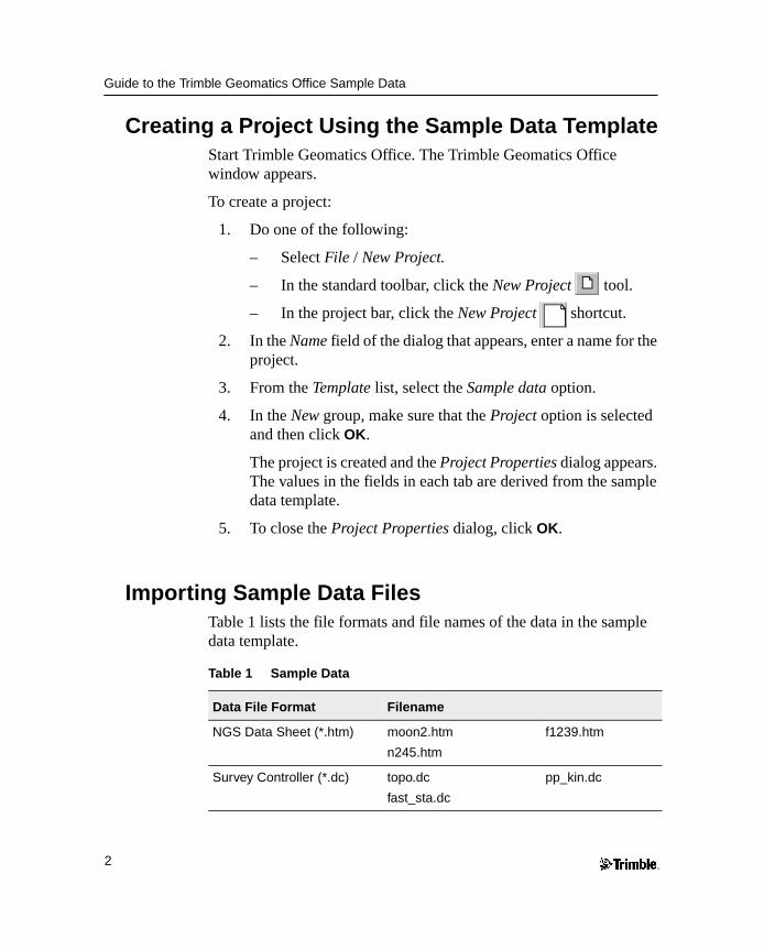
National Geodetic Survey (NGS) Data Sheet files are files that contain coordinates for survey monuments in the United States of America. This section describes one way to import control information.

To import these files into your sample data project:

1. Open the Import dialog. To do this, do one of the following:

– Select File / Import.

– Select the Import tool.

2. In the Survey tab of the dialog that appears, select the NGS data sheet file (*.dat,*.dsx,*.htm,*.html,*.prl) option.

3. Click OK. The following dialog appears:

The Look in field defaults to the project’s Checkin folder.

4. Highlight the moon2.htm, n245.htm, and f1239.htm files to import. (To select multiple files, press [Ctrl] .)

5. Click Open.

4


The software imports the NGS data files and stores them in the default folder for the project. It imports the control points for the moon2, n245, and f1239 files, which you can see in the Survey view. The triangle symbol for the moon2 file shows that it is a 2D control point. The square symbols for the n245 and f1239 files show they are 1D control points (only the elevation is of control quality).

Labeling the points

To show the names of the points on the screen:

1. Select Select / All.

2. Select View / Point Labels. The Point Labels dialog appears.

3. In the Label Points with field, select the Name check box and then click OK.

The points are labeled with their names.

Importing Control CoordinatesYou can also import control coordinates from a text file into your project. To do this:

1. Select File / Import to open the Import dialog.

2. In the Custom tab, select the Name, North, East, Elevation, Code option.

3. Click the Options buttons and make sure that the Settings tab is selected.

4. In the Quality for Import data field, select Control quality to ensure that the points you are about to import will have a control quality.

5. Click OK. The Open dialog appears. The Look in field defaults to the project’s Checkin folder.

6. Highlight the Control Coordinates.csv file and click Open.

The software imports the Control Coordinate file and stores it in the Data Files folder for the project.

5


Importing GPS Data (*.dat) Files

Using the GPS Data files (*.dat) option in the Import dialog, import the following files:

• fast0550.dat

• Ktom0550.dat

• Moon0550.dat

• Wave0550.dat

When you import GPS Data files, the DAT Checkin dialog appears. This dialog shows information about the imported GPS files. Click OK to import the .dat files.

The unprocessed baselines are displayed in the Survey view.

Use the steps outlined in Labeling the points, page 5, to label the GPS points.

Note – You can view a project in the Survey view or the Plan view. Use the Survey view when performing survey-related tasks, and the Plan view to view topographic features observed during the field survey.

Processing GPS BaselinesTrimble Geomatics Office includes the WAVE™ (Weighted Ambiguity Vector Estimator) baseline processor and Timeline. The WAVE baseline processor computes baseline solutions from GPS field observations made using static, FastStatic, or kinematic data collection procedures. Timeline displays GPS data found in raw observation files in a graphical, time-based format. Timeline is only available in the Survey view.

This section describes how to:

• use the WAVE Baseline Processor to process GPS baselines

• evaluate processed results

• examine observations in Timeline

6


Note – The functionality described in this section is only available if the WAVE baseline processing module is installed.

Processing Potential Baselines

To process all potential baselines, do the following:

1. To ensure that no baselines are selected, do one of the following:

– Select Select / None.

– Click on a blank area of the screen.

2. To start the WAVE baseline processor, do one of the following:

– Select Survey / Process GPS Baselines.

– In the project bar, in the Trimble Survey or Process groups, click the Process GPS Baselines shortcut.

7


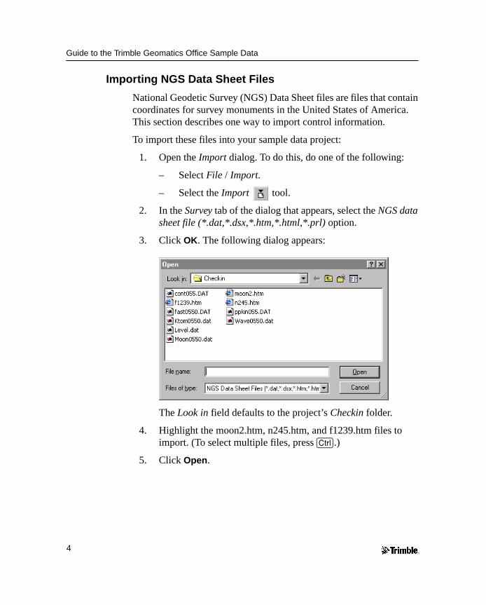
The GPS Processing dialog appears.

Initially, the status bar in the bottom left corner of the dialog shows the files being loaded for processing. When the actual processing begins, the status bar shows the From and To stations and results are added to the table as they are completed. The processor then continues with the next baseline until all processing is complete, as shown below:

In its right corner, the status bar now displays a summary of the number of baselines accepted (Acc) and rejected (Rej).

3. Click Save to save the processed GPS baselines.

Use the steps outlined in Labeling the points, page 5, to label the GPS points that have just been processed.

8


Figure 1 shows the processed GPS baselines.

Figure 1 The GPS baselines

9


Evaluating Results

To examine the point WAVE:

1. Double-click the point WAVE in the center of the network. The following Properties window appears:

The Properties window lets you view the details of all entities (points, observations, lines, arcs, curves, text, annotations). Use it whenever you want to view and edit entity details.

To open the Properties window at any time, do one of the following:

– Select Edit / Properties.

– In the standard toolbar, click the Edit Properties tool.

– Double-click a graphical entity.

– Press [Alt]+[Enter] .

When the Properties window is open, you can view an entity’s details by clicking on it in the graphics window.

In the Properties window, the Summary page shows the coordinates and coordinate quality for the point WAVE. (To access this page, click .)

10


2. Expand the tree on the left-hand side of the Properties window to view the observations and keyed-in coordinates for the point WAVE.

3. The Point Derivation report shows how a recomputation determined the calculated position for the point WAVE. To view the report, select .

4. The Point Derivation report appears. In this case, the NEe coordinate in the control coordinates text file was adopted. The height was derived from the geoid model.

5. Close the report.

Viewing the GPS Baseline Processing report

To view the GPS Baseline Processing report for the baseline from MOON 2 to WAVE:

1. Select the baseline from MOON 2 to WAVE. In the Properties window, do the following:

a. Make sure that WAVE is still selected.

b. In the left pane, click the plus sign (+) next to the point name WAVE to show all of the observations for the point.

c. Select MOON 2-WAVE.

2. Select Reports / GPS Baseline Processing Report.

The GPS Baseline Processing report appears. Scroll through the report to view the baseline summary, the baseline components, and the tracking summary.

The report lets you assess whether the baseline processing has been successful, and check the entered field data. For example, you can check the satellite residuals.


11


Using Timeline

You can use Timeline to examine the data for the baseline from MOON 2 to WAVE:

1. To start Timeline, do one of the following:

– Select View / Timeline.

– Select .

Timeline appears below the Survey map area of the graphics window. Horizontal bars represent the data collected by each GPS receiver. If a bar is broken into segments, this shows that it has multiple occupations.

The Timeline and Plot toolbars also appear, as shown below:

B Tip – The Survey map area and Timeline are both part of the graphics window. To show more or less of Timeline, raise or lower the bar separating Timeline from the Survey map area.

2. In the Properties window, select the baseline from MOON 2 to WAVE.

The time in the Properties window shows that the baseline from MOON 2 to WAVE was observed for 8 minutes, from 7:11:02 on the 25th February 1999.

3. Enlarge Timeline so that it covers half of the graphics window.

12


Figure 2, shows the base receiver (MOON 2) and the roving receiver (WAVE) segments for the baseline. The bottom half of the observation segment bar is highlighted in a different color.

Figure 2 Timeline

4. In the file 4800:20116954, in the highlighted data segment, right-click to access the shortcut menu, and then select Zoom to Span. The data segment widens along the Timeline screen.

5. To expand the file, click the plus sign (+). This shows the satellites that were observed at WAVE.

6. To view the elevation data for satellite 26:

a. On SV 26, right-click to access the shortcut menu, and then select SV Plot. The Timeline-GPS Signal Plots window appears. You can use this window to view information about the satellites that were observed. For example, you can view the L1 and L2 signal-to-noise (SNR) ratios, the satellite azimuth, and the elevation.

b. Close the Timeline-GPS Signal Plots window.

WAVEMOON 2

13


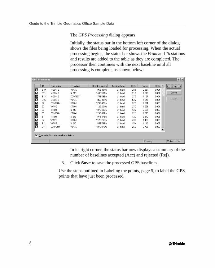
7. To view information about each observation, double-click on an observation segment. The GPS Observation Properties dialog appears.

Note – If your GPS observations contain cycle slips, you can disable them. Drag a box around the cycle slip, then right-click to access a shortcut menu and select Disable, as shown below:

8. To close Timeline, select View / Timeline.

For more information about Timeline, refer to the Trimble Geomatics Office User Guide.

14


GPS Loop ClosuresTo check the quality of, and identify any errors in, a set of GPS observations within a network, you can perform loop closures and then view the GPS Loop Closures report.

To set up the information to be displayed in the GPS Loop Closures report:

1. Select Reports / Setup / GPS Loop Closures Report. The Loop Closure Settings dialog appears.

2. In the Tolerance group, set the horizontal and vertical tolerance.

3. In the Report Sections group, select the sections to be displayed in the report.

To view the GPS Loop Closures report:

1. Select Reports / GPS Loop Closures Report. If you have observations selected, the Loop Closure Report dialog appears:

– In the Report on group, select the Whole database option and then click OK. The GPS Loop Closures report appears.

In the Summary section, the number of failed loops is 0. This shows that the GPS baseline loops close within the set tolerance, and that the data is ready for a network adjustment.


15


Performing a Minimally Constrained Adjustment of GPS Data

A minimally constrained adjustment is an adjustment with only one control point, which is held fixed in the survey network. This section describes how to:

• display the Ellipse Controls

• select the adjustment datum

• fix a point in the network

• perform a minimally constrained network adjustment

• view the adjustment results

Note – You can only perform a network adjustment if you have purchased the Network Adjustment module.

Setting up the project for minimally constrained adjustment for GPS data

The following sections show how to perform a minimally constrained adjustment of GPS data.

Display the ellipse controls

To display the Ellipse Controls toolbar, do one of the following:

• Select View / Toolbars / Ellipse Controls.

• Right-click on the Trimble Geomatics Office toolbar to access the shortcut menu, and then select Ellipse Controls.

In the toolbar, select the Error Ellipse tool to show the ellipses when the adjustment is performed.

16


Set the WGS-84 datum

To perform a minimally constrained adjustment of GPS data, select the WGS-84 datum.

To do this:

• Select Adjustment / Datum / WGS-84.

Set the adjustment style

You can set up the adjustment style to suit your project. In this example, use the 95% confidence limits for the adjustment style. To do this:

1. Select Adjustment / Adjustment Styles. The Network Adjustment Styles dialog appears.

2. In the Network Adjustment Styles dialog, select 95% Confidence Limits from the list and then click Edit.

3. In the 95% Confidence Limits dialog, select the Set-up Errors tab.

4. In the GPS group, do the following:

– In the Error in Height of Antenna field, enter 0.003.

– In the Centering Error field, enter 0.002.

5. In the Terrestrial group, do the following:

– In the Error in height of Instrument field, enter 0.003.

– In the Centering Error, enter 0.002.

6. To close each dialog, click OK.

17


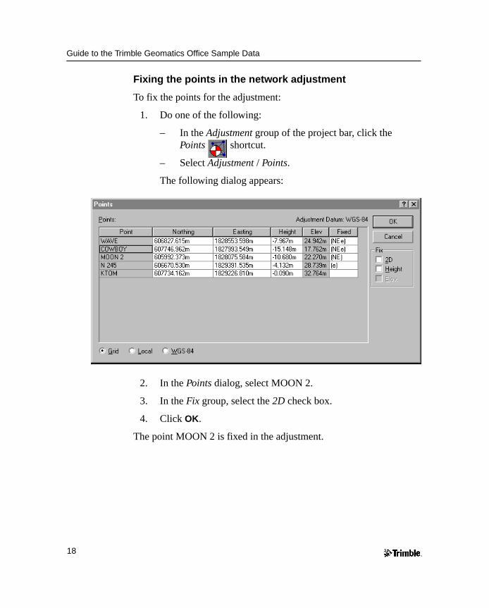
Fixing the points in the network adjustment

To fix the points for the adjustment:


– In the Adjustment group of the project bar, click the Points shortcut.

– Select Adjustment / Points.

The following dialog appears:

2. In the Points dialog, select MOON 2.

3. In the Fix group, select the 2D check box.

4. Click OK.

The point MOON 2 is fixed in the adjustment.

18


Performing a Minimally Constrained Adjustment

To perform the adjustment, do one of the following:

– Select Adjustment / Adjust.

– In the Adjustment group of the project bar, click the Adjust shortcut.

Error ellipses will appear in the Survey view.

Viewing the Adjustment Results

To view the results of the adjustment, you need to view:

• the Network Adjustment report

• the Observations dialog

The following sections describe each task.

Viewing the Network Adjustment report

To view the Network Adjustment report:

1. Select Reports / Network Adjustment Report. The Network Adjustment report appears.

2. Maximize the report and in the Contents section, click Statistical Summary. (This summary is an important tool for analyzing the adjustment.)

The Chi-square test shows how well your observations fit together. However, in this adjustment, the Chi-square test fails. The network reference factor shows how well the observation errors are estimated. In this case, it exceeds 1.0.


When the Chi-square test fails and the network reference factor exceeds 1.0, this shows that the estimated observational errors are underestimated and do not match the amount of adjustment made to the observations.

19


There are two options:

• Check to see that there are outliers in your data.

• Apply a scalar to the estimated errors to model the observation errors more accurately. (For more information, see Applying a Scalar to the Estimated Errors, page 21.)

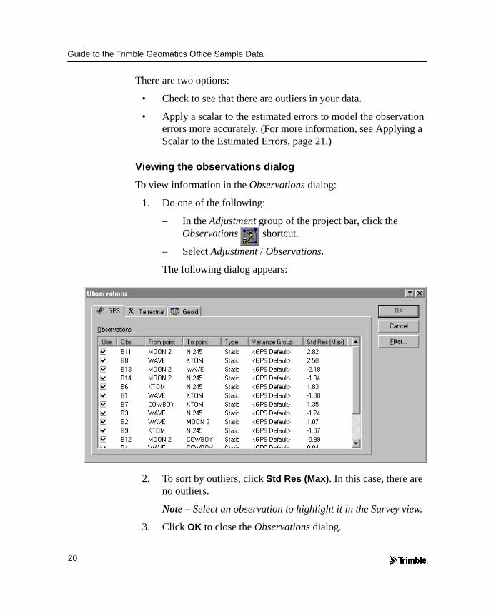
Viewing the observations dialog

To view information in the Observations dialog:


– In the Adjustment group of the project bar, click the Observations shortcut.

– Select Adjustment / Observations.


2. To sort by outliers, click Std Res (Max). In this case, there are no outliers.

Note – Select an observation to highlight it in the Survey view.

3. Click OK to close the Observations dialog.

20


Applying a Scalar to the Estimated Errors

To apply a scalar to the estimated errors:

1. Select Adjustment / Weighting Strategies. The Weighting Strategies dialog appears.

2. Make sure that the GPS tab is selected.

3. In the Scalar Type group, select the Alternative option.

Using the alternative scalar strategy for the second adjustment automatically multiplies the first scalar value (1.0) by the current adjustment network reference factor value.

4. Click OK.

5. To readjust the network, select Adjustment / Adjust.

6. To view the Network Adjustment report, select Reports / Network Adjustment report.

7. Maximize the report and in the Contents section, click Statistical Summary.

During the second adjustment, the new scaled estimated errors are applied. The Chi-square test still fails.


9. You can automate the process of applying a scalar to the estimated errors, using the automatic scalar option. To do this:

a. Select Adjustment / Weighting Strategies. The Weighting Strategies dialog appears.

b. Make sure that the GPS tab is selected.

c. In the Scalar Type group, select the Automatic option.

d. Click OK.

The software performs an automatic adjustment, using the Alternative scalar type option. It repeats this adjustment until the global statistics are acceptable; that is, until the Chi-square test passes. For more information, refer to the Help.

21


10. Readjust the network and view the Network Adjustment report. The Chi-square test should now pass.

11. Close the Network Adjustment report.

Note – When you have finished performing a minimally constrained adjustment on the GPS data, you can save coordinates for a calibration by selecting Adjustment / Calibration Coordinates / Save.

Adjusting Terrestrial DataTrimble Geomatics Office supports the adjustment of terrestrial data, as well as GPS data. To include terrestrial data in an adjustment, you need to do the following:

1. Import terrestrial data.

2. Investigate any error flags.

3. Change to the adjustment datum.

4. Load geoid observations.

5. Perform a minimally constrained adjustment on the terrestrial data.

6. View the network adjustment report.

22


Importing Terrestrial Data

The terrestrial data set that is used in the sample data is called Topo.dc.

To import it:


2. In the Survey tab, select the Survey Controller files (*.dc) option.


4. Highlight the Topo.dc file.

5. Click Open.

The software imports the file and stores it in the Data Files folder for the project.

Leveling observations or delta elevations often form part of the terrestrial adjustment network. You can also use them to improve the elevations derived from GPS observations. There is a Digital Level file included with the sample data. To import data from a Digital Level file:


2. In the Survey tab, select the Digital Level files (*.dat, *.raw) option.


4. Highlight the Level.dat file.

23


5. Click Open. The following dialog appears:

The Digital Level Import dialog does the following:

– Displays the data from a Digital Level file

– Determines which points are used to compute delta elevations. (Delta elevations are only computed between points selected as station points).

– Shows the elevation of the starting point. The starting point is represented by the symbol .

For more information, refer to the Help.

6. To make sure that only the station points are imported into the project, click Select by Filter. The Define Level Stations dialog appears.

7. Select the Select points with option.

8. Make sure that the Description list shows STN* and then click OK. In the Digital Level Import dialog, the points that are not station points will be cleared.

24


9. Click OK. The Digital Level file is imported.

Note – Editing the data in the Digital Level Import dialog does not edit the digital level file.

To view the digital level observations in the Properties window:

1. Select Select / Observations. The Select Observations dialog appears.

2. From the Type list, select the Delta Elevations check box and then click OK.

3. To open the Properties window, do one of the following:

– Select Edit / Properties.

– In the standard toolbar, click the Edit Properties tool.

– Press [Alt]+[Enter] .

When the Properties window is open, click on a specific level observation to view its details.

4. Close the Properties window.

Investigating Error Flags

When you import Topo.dc, error flags appear in the data. To investigate them, do one of the following:

• Double-click on the error flags in the graphics window.

• Double-click on the error flag shown in the status bar.

If you use the Flag icon in the status bar, all points with error flags appear in the Properties window.

To investigate these flags, you can view the point information in the Point Derivation report.

On point 1000, the flag is caused by the elevation and height on two check observations being out of tolerance. These two check observations do not match the enabled observation. This indicates that there may be something wrong with the observation.

25


To investigate it:

1. In the Point Derivation report for point 1000, click the hyperlink (the satellite icon) for the enabled observation and minimize the report. The observation is selected in the Properties window.

2. In the Properties window, select the rover Occupation page, as shown below:

3. The antenna height is 1.900. In this example, it should be 1.800.

4. In this page, change the antenna height to 1.800 and press [Enter]. The antenna height is changed.

5. To recompute the data, do one of the following:

– Select Survey / Recompute.

– Press [F4].

6. The flag on point 1000 is removed.

Note – At this stage you can check that other antenna height blunders do not occur in the data. To change all of the 1.900 meter antenna heights to 1.800 meters, use the Multiple Edit dialog.

26


Adjusting Terrestrial Observations

The following sections show you how to adjust terrestrial observations.

Note – In this sample data, there is not enough redundancy in the level data to perform the minimally constrained terrestrial adjustment without the GPS data present. In some cases, you may have enough redundancy to remove your GPS data before performing a minimally constrained terrestrial adjustment.

Setting the adjustment datum

To perform a minimally constrained adjustment on terrestrial observations, you will need to change the datum to the project datum. To do this:

• Select Adjustment / Datum / Project Datum – NAD 1983 Conus.

Create a variance group for level observations

To create a separate variance group for the level observations in the adjustment, do the following:

1. Select Adjustment / Observation Groups / Variance Groups. The Variance Group dialog appears.

2. In the Terrestrial tab, click New. The New Variance Group dialog appears.

3. In the Name Group, enter Level Observations and then click OK. The Edit Variance Group dialog appears.

4. Click Filter. The Observation Filter dialog appears.

5. Clear all of the check boxes except Delta elev and click OK to return to the Edit Variance Group dialog.

6. In the Available Observations group, select the delta elevations observations and click Add. The delta elevation observations now appear in the Group observations field.

27


7. Click OK to return to the Edit Variance Group dialog.

8. Click Close.

Remove sideshots from the adjustment

The following example shows how to remove side shots from the adjustment:

1. To select the sideshot observations:

a. Select Select / Observations. The Select Observations dialog appears.

b. Make sure that the General tab is selected.

c. In the Type list, select the Terrestrial – Single face only check box.

d. Select the Side shots only check box.

e. Click OK.

The terrestrial sideshot observations are selected.

2. To remove the sideshot observations from the adjustment:

a. Select Edit / Multiple Edit. The Multiple Edit dialog appears.

b. In the Perform these edits to the selected observations group, select the Use in Network Adjustment option.

c. From the Use in Network Adjustment list, select No.

d. Click OK.

The sideshot observations will not be used in the network adjustment.

B Tip – You can also remove the sideshot observations from the adjustment using the Terrestrial tab in the Observations dialog. To do this, clear the Use check box for a highlighted observation. The Use check box for all of the other selected observations will also be cleared.

28


At this point in the adjustment, you will also need to load geoid observations so that the relationship between elevations (from terrestrial observations) and ellipsoid heights (from GPS observations) can be established.

Loading geoid observations

To load geoid observations:

1. Select Adjustment / Observations. The Observations dialog appears.

2. In the Geoid tab, click Load. The geoid observations are loaded into the Observations group.

3. Click OK. You are now ready to fix a point in the network.

Fixing the points in the network

To fix the points for the adjustment:


– In the Adjustment group of the project bar, click the Points shortcut.

– Select Adjustment / Points.

29



2. Select MOON 2, and in the Fix group, select the 2D check box.

3. Select N245, and select the Elev. check box.

4. Select F1239, and select the Elev. check box.

5. Click OK.

Adjust

To perform the adjustment, do one of the following:

• Select Adjustment / Adjust.

• In the Adjustment group of the project bar, click the Adjust shortcut.

30


Viewing the Network Adjustment report

To view the Network Adjustment report:

1. Select Reports / Network Adjustment Report. The Network Adjustment report appears.

2. Maximize the report and in the Contents section, click Statistical Summary. (This summary is an important tool for analyzing the adjustment.)

The Chi-square test shows how well your observations fit together. The network reference factor shows how well the observation errors are estimated. In this case, the Chi-square test passes.

Note – You should also view the terrestrial observation statistics.


Scaling the errors

To scale the standard errors:

1. Select Adjustment / Weighting Strategies. The Weighting Strategies dialog appears.

2. Make sure that the Terrestrial tab is selected.

3. In the Apply Scalars To group, select the Variance Groups option.

4. In the Scalar Type group, select the Automatic option.

5. Click OK.

6. Select Adjustment / Adjust to readjust the network and then view the Network Adjustment report.

31


7. To scale the geoid observations:

a. Before scaling the geoid observations, you need to fix elevations. In the Points dialog, fix the elevations of the points N 245, WAVE, DON, and F 1239.

b. In the Weighting Strategies dialog – Geoid tab, select the Alternative scalar type option.

8. Select Adjustment / Adjust to readjust the network and then view the Network Adjustment report.

9. Click OK.

Performing a Fully Constrained AdjustmentYou can now perform a fully constrained adjustment.

To do this:

1. Make sure that the adjustment datum is still set on the project datum.

2. You now need to generate the necessary transformations by constraining (fixing) the control points you have chosen to use in your network. The control points are usually well-established survey marks with high-accuracy horizontal (2D) or vertical coordinates.

3. To do this:

a. In the Points dialog, fix the following points:

– MOON 2 – NE

– N 245 – e

– WAVE – NEe

– DON – NEe

– F 1239 – e

b. Click OK.

32


Note – Perform an adjustment after fixing each point. This lets you check that each point is not contributing to errors in the adjustment.

4. Select Adjustment / Adjust to perform a fully constrained adjustment.

5. Select Reports / Network Adjustment Report to view the Network Adjustment Report. The Network Adjustment report appears.

6. View the information in the Statistical Summary section. The Chi-square test passes, indicating a successful adjustment. You can now view the adjusted coordinates for the file.

7. Close the Network Adjustment report.

8. In the toolbar, select the Error Ellipse tool to turn off the ellipse display.

For more information about network adjustments, refer to the Trimble Geomatics Office User Guide.

33


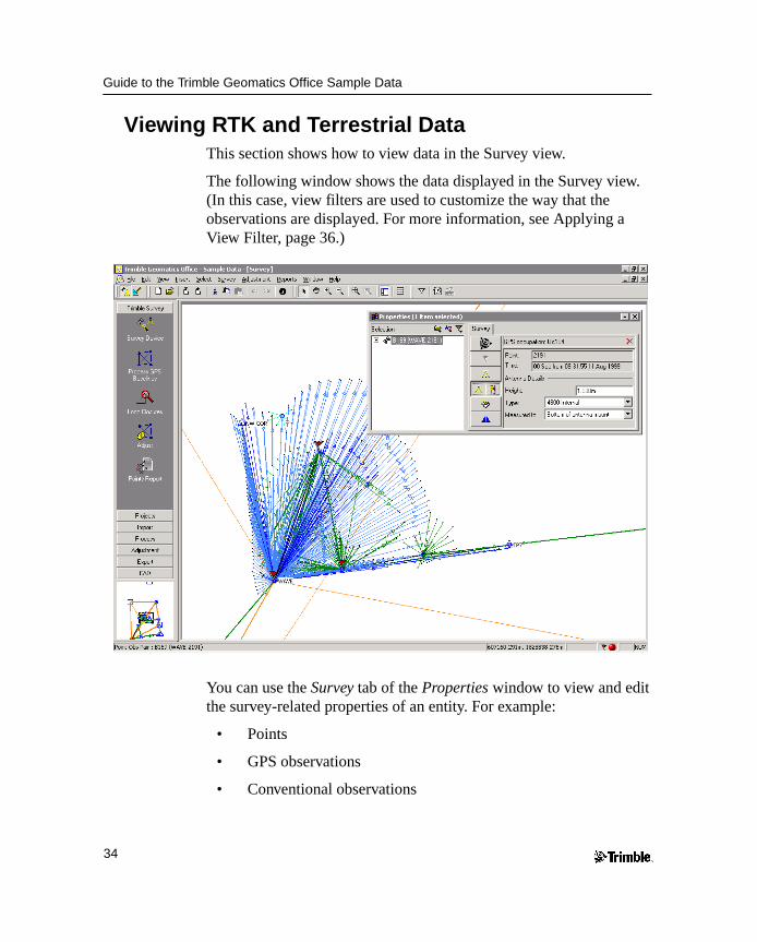
Viewing RTK and Terrestrial DataThis section shows how to view data in the Survey view.

The following window shows the data displayed in the Survey view. (In this case, view filters are used to customize the way that the observations are displayed. For more information, see Applying a View Filter, page 36.)

You can use the Survey tab of the Properties window to view and edit the survey-related properties of an entity. For example:

• Points

• GPS observations

• Conventional observations

34


• Laser rangefinder observations

• Reduced observations

• Level observations

• Azimuth observations

In the window on the previous page, the observations at the bottom left of the screen were collected conventionally because overhead obstructions prevented the collection of GPS data. Double-click on a conventional observation to display it in the Properties window, as shown below:

This Properties window shows the instrument setup details for the conventional observation from points 1001 to 2305. Use the Target setup and Observation data page buttons to examine the target setup details and the observation components between the instrument and target setups.

Use the Properties window to view the survey-related properties of other entities, such as laser rangefinder observations.

35


Applying a View Filter

You can use a view filter to change the way the observations are displayed in the Survey view. To apply a view filter:


– Select the View Filters tool.

– Choose View / Filters.

– Press [Ctrl]+[F].


2. To select the types of observations that you want to view, select an option from the Observations group. For example, select the Show all observations option to enable all observation types to be selected for viewing.

36


Note – The Show only observations marked for adjustment and Show only observations able to be adjusted options are only available if you have the Network Adjustment module installed.

The check boxes in the Types of observations to show group vary according to the option selected. The upper group displays the observation types that can be selected for viewing. The lower group displays the properties for the observation types (where applicable).

3. In the Types of observations to show group, do the following:

a. Select the check boxes from the upper group to select the observation types that you want to view.

b. Select the appropriate check boxes from the lower group to display only the observation types (selected in the upper group) with those properties.

Note – You can only use the check boxes in the lower group if you have specified an observation type for the upper group.

Once a filter is applied to a project, the View Filters are on icon appears in the status bar. You can double-click this icon to access the View Filters dialog and make any changes to the filters.

Note – The view filters remain applied even after you close and then reopen a project.

For more information on using the Survey view and applying a view filter, refer to the Trimble Geomatics Office User Guide.

37


Viewing Grid Lines

Grid lines in the graphics window show the scale of the project. They can help you to easily find particular coordinate locations.

To show grid lines in the graphics window, do the following:

1. Select View / Options. The following dialog appears:

2. In the Grid Lines tab, select the Show grid lines check box. You can display:

– A fixed number of grid lines – the same number of grid lines will be displayed when you zoom in and out.

– Grid lines at the interval that you specify – the number of grid lines displayed is increased or decreased depending on whether you zoom in or out.

3. Select an appropriate line type and color from the Grid line type and Grid line color lists.

4. If necessary, label the grid lines by selecting the Label grid lines check box.

38


B Tip – You can also display the grid lines in the graphics window by selecting the Grid Lines tool in the toolbar.

Viewing Background Maps

Trimble Geomatics Office can display Background Map files in the graphics window. You can import Drawing exchange format (.dxf), Windows bitmap (.bmp), or Tagged Image File Format (.tif) files to display. These files must be georeferenced, using ESRI’s World file format, to be displayed correctly.

A World file is an ASCII text file with a .tfw or .wld extension. To be used in Trimble Geomatics Office, the World file must:

• use the same coordinate system as your project

• have the same units as your project

Note – The rotation in the World file is not used in Trimble Geomatics Office.

To select a Background Map file to display:

1. Select View / Options. The View Options dialog appears.

2. In the Background Map tab, click Add. The Add dialog appears.

3. Select halfmoon.bmp and click Open. The file appears in the File names list in the Background Map tab.

4. Click OK. An aerial photo image appears in the background of the graphics window.

To remove the image:

• In the Background Map tab, select the file and click Remove.

For more information about Background Map files, refer to the Help.

39


Feature Code ProcessingThis section describes how to process feature codes. You can process any points that have feature codes assigned to them.

To process feature codes:

1. Switch to the Plan view. To do this, do one of the following:

– In the toolbar, select the Plan View tool.

– Select View / Plan.

2. In the Plan view, select Tools / Process Feature Codes. The following dialog appears:

3. In this example, use the Default.fcl feature and attribute library that appears in the dialog. However, you can click Browse and use the Browse dialog to locate and select the feature and attribute library with which you want to process feature codes.

4. In the Process group, select the Topo.dc selection set.

Note – You must choose a selection set created from the imported .dc file, not the current group of selected points. This ensures that the points are processed in the order in which they are collected. If you select points using any other selection method, unexpected feature code processing can occur.

5. Click OK to start processing feature codes.

40


The following window shows the zoomed results of the feature code processing:

After feature code processing, the Plan view graphically shows the area that was surveyed. (Note that conventional observations were made in an area where there are a lot of trees.)

The sample data also has feature and attribute information.

To view attributes:

1. Double-click a point feature. The Properties window appears.

2. Select the Attributes tab. It shows the attributes for the currently selected feature.

You can export attributes to a number of popular GIS software formats. For more information, refer to the Help.

41


In the Plan view you can also do the following:

• Create, edit, and delete:

– Layers

– CAD styles

– Annotation templates

• Add lines, curves, arcs, text, and annotations

For more information on using the Plan view, refer to the Trimble Geomatics Office User Guide.

Exporting DataThis section shows how to export the project as an AutoCAD .dxf file.

To create a .dxf file from your project:


– Select File / Export.

– Click the Export tool.

The Export dialog appears.

2. Select the CAD / ASCII tab.

B Tip – You can configure the format of the DXF/DWG file by clicking Options.

3. Select the AutoCAD files (*.dxf/*.dwg) option and click OK. The Save As dialog appears.

4. Locate the folder you want to export the file to.

5. In the File Name field, enter a name and then click Save.

The software creates the file in the folder that you selected.

42


Further InformationThis document uses the sample data to show some of the functionality of Trimble Geomatics Office. There are also other files that can be easily imported and viewed.

For more information, refer to the Trimble Geomatics Office User Guide.

Copyright

© 2000–2002 Trimble Navigation Limited. All rights reserved. The Globe & Triangle logo with Trimble, Trimble Geomatics Office, and WAVE are trademarks of Trimble Navigation Limited. The Sextant logo with Trimble is a trademark of Trimble Navigation Limited, registered in the United States Patent and Trademark Office. All other trademarks are the property of their respective owners.

43


44

guide to the trimble geomatics office sample...

Documents