FEDERAL RESERVE BANK OF SAN FRANCISCO

WORKING PAPER SERIES

Government Consumption Expenditures and the Current Account

Michele Cavallo Federal Reserve Bank of San Francisco

February 2005

Working Paper 2005-03 http://www.frbsf.org/publications/economics/papers/2005/wp05-03bk.pdf

The views in this paper are solely the responsibility of the authors and should not be interpreted as reflecting the views of the Federal Reserve Bank of San Francisco or the Board of Governors of the Federal Reserve System.

ABSTRACT

This paper distinguishes between two components of government consumption, expenditure on final

goods and expenditure on hours, and compares the effects of changes in these two on the current

account. I find that changes in government expenditure on hours do not directly affect the cur-

rent account and that their impact is considerably smaller than the impact produced by changes

in government expenditure on final goods. These findings indicate that considering government

consumption as entirely expenditure on final goods leads to overestimating its role in accounting for

movements in the current account balance.

keywords: Government expenditure; Government hours; Current account

jel classification codes: E60; E62; F41

∗Economic Research Department, 101 Market Street, Mail Stop 1130, San Francisco, CA 94105; Tel.: 415-974-3244;

Fax: 415-974.2168. I thank Darrel Cohen for encouragement to work on this topic; Fabio Ghironi, Reuven Glick,

Nouriel Roubini, Mark Spiegel and Diego Valderrama for helpful conversations; Judith Goff and Anita Todd for

editorial assistance; and Greg Snyders for excellent research assistance. All remaining errors are my own. The views

in this paper are solely my responsibility and should not be interpreted as reflecting the views of the Federal Reserve

Bank of San Francisco or the Federal Reserve System.

1 Introduction

The current account balance is the difference between a country’s exports and its imports of

goods, services, and income. It also measures the difference between a country’s national income

and its domestic expenditure on consumption and investment. A considerable share of domestic ex-

penditure in industrialized countries consists of government consumption expenditure. For example,

in the United States, government consumption expenditure after World War II has accounted, on

average, for roughly 20 percent of total domestic expenditure. Previous studies have therefore ex-

amined the relation between changes in government consumption expenditure and movements in the

trade balance on goods and services, whose short-run fluctuations, as highlighted in Baxter (1995),

track closely those of the current account balance. Among those studies, Ahmed (1987) found some

evidence of a negative relationship between temporary increases in government expenditure and the

trade balance for the United Kingdom during the 18th and the 19th centuries. Likewise, Yi (1993)

showed that higher government purchases played at least a partial role in the deterioration of the

U.S. trade balance during the 1970s and 1980s.

Government consumption expenditure consists of two main components: expenditure on final

goods, and wage and salary accruals, which, essentially, correspond to expenditure on hours worked.

Figures 1A and 1B indicate that the latter component has represented a quantitatively relevant share

of both GDP and government consumption expenditure for the United States during the post-World

War II period. Moreover, within a model economy, as shown by Finn (1998), government expenditure

on hours has a negative impact on domestic output and investment expenditure in the private sector,

whereas government expenditure on final goods has a positive impact (see, e.g., Baxter and King,

1993).

This paper, therefore, explores the dynamic effects of unanticipated increases in government

expenditure on both final goods and hours, using a two-country model economy. In particular,

it compares the consequences for the current account of a shock to government hours with those

produced by a shock to government expenditure on final goods. The main results are as follows.

An increase in government expenditure on final goods corresponding to 1 percent of GDP produces

on impact a deterioration in the current account balance of nearly 0.5 percent of GDP, as in Baxter

(1995). More notably, this paper also shows that an equivalent increase in government expenditure

on hours produces a considerably smaller deterioration in the current account balance, corresponding

to barely 0.05 percent of GDP.

While an increase in government expenditure of final goods is accommodated through higher

imports, an increase in government hours is accommodated by an expansion in domestic labor

supply. In the former case, there is a corresponding deterioration in the trade and current account

balances, whereas, in the latter, there are no direct consequences on net exports of goods, services,

and income. Similarly, since hours worked are nontraded, an increase in government hours does not

directly affect the excess of domestic expenditure over national income. As a result, it does not lead

directly to a deterioration in the current account. However, it still has an indirect effect, though

quantitatively smaller, on the current account through its impact on domestic private output and

expenditure on consumption and investment.

These results indicate that it is important to consider the composition of changes in gov-

ernment consumption expenditure to understand their impact on the current account balance. In

addition, they hint that a fiscal deficit generated by an increase in government expenditure on hours

has a substantially smaller impact on the current account than a fiscal deficit generated by an

increase in government expenditure on final goods. Instead, most theoretical models, like the two-

country model in Baxter (1995), predict that a fiscal deficit generated by an increase in government

consumption expenditure produces a sizeable deterioration in the current account balance. In the

United States, government expenditure on hours has accounted for a substantial share of govern-

ment consumption expenditure, as illustrated in Figure 1B. Taking this into account, the results

of this paper bring the predictions of a model economy about the association between fiscal and

current account deficits closer to the recent findings of Kim and Roubini (2004). Their evidence, in

fact, show that increases in the fiscal deficit actually improve the current account to some extent.

In a related paper, Erceg, Guerrieri and Gust (2005) have used a two-country model—

calibrated to the U.S. economy and to the rest of the world—with nominal and real rigidities and

with financial imperfections. They have found that fiscal deficits have only a fairly small effect on the

U.S. trade balance. For example, a fiscal deficit generated by an increase in government expenditure

on final goods which is equivalent to 1 percent of GDP induces a trade balance deterioration that

is smaller than 0.2 percent of GDP.

The structure of the paper is as follows: Section 2 presents the model economy. Section 3

describes the solution of the model. Section 4 illustrates and discusses the dynamic responses to

unanticipated increases in government consumption expenditures. Section 5 briefly concludes.

2

2 The model economy

The model economy consists of two countries, home and foreign, of size π and (1 − π) ,

respectively. In each country there is a household sector, a private sector, and a government. In

the household sector there is a large number of households. In the private sector there is a large

number of identical firms. Both domestic and foreign firms produce a single final good that can be

used for either consumption or investment purposes and that can be freely traded between the two

countries. The set of financial claims includes a single noncontingent bond, denominated in units of

the final good, and equity claims on the dividend stream of private sector firms. The first type of

claims can be traded internationally, while the latter cannot.

As in Ghironi (2003), I use an overlapping-generations (OLG) version of the two-country

general equilibrium model, rather than the representative agent version. In the representative agent

framework, when the set of internationally traded financial claims includes only noncontingent

bonds, insurance against country-specific shocks is incomplete. This implies that these shocks, even

when temporary, produce permanent changes in the distribution of wealth across countries and in

the levels of the other endogenous variables, thereby modifying the long-run equilibrium of the model

economy. It is therefore problematic to analyze the dynamic effects of temporary country-specific

shocks through solution techniques that are valid only around an equilibrium to which variables

eventually return. In contrast, in the OLG framework, temporary country-specific shocks do not

alter the long-run equilibrium of the model economy. After these disturbances, as newly born

households with zero financial wealth enter the economy at the beginning of each period, aggregate

per capita levels of wealth and of the other endogenous variables eventually return to their preshock

equilibrium values.

Finally, time is divided into periods and each period is indexed by the subscript t.

Households

Households consume final goods and supply labor services in the form of hours worked both to

private sector firms and to the government. These labor services are perfectly mobile across sectors

within the same country but immobile across countries. For simplicity, I normalize the households’

endowment of hours to one. As in Blanchard (1985), Frenkel, Razin, and Yuen (1996, Ch. 9) and

Cardia (1991), in each period households face a constant probability of death, denoted by (1 − ϕ) .

As a consequence, the probability of survival from one period to the next is ϕ. The representative

household in the home country born on date v has preferences over consumption Ct,v and hours

3

worked Nt,v. These preferences are represented by the following utility function:1

∞∑i=0

(ϕβ)i U(Ct+i,v, Nt+i,v),(1)

where β is the subjective discount factor. The momentary utility function is

U(Ct,v, Nt,v) = θ log Ct,v + (1 − θ) log (1 − Nt,v) , 0 < θ < 1.(2)

Households supply labor hours in a perfectly competitive labor markets. The real wage per hour

unit is Wt. Households also pay lump-sum taxes, Tt. They hold equity claims on the profit stream

of private sector firms. I denote these claims by St,v, their price by Vt, and the profits paid out in

period t by Dt. They also hold a noncontingent real bond, Bt,v, that earns a gross real interest rate

of Rt.

Households stipulate contracts with insurance companies contingent on survival. These con-

tracts establish that, in the event of death, holdings of financial claims—bonds and equity claims—

are transferred to insurance companies. Alternatively, in the event of survival, insurance companies

pay households an extra return on their assets. With free entry into the insurance market, a zero

profit condition determines the extra return. This condition implies that insurance companies allo-

cate to those who remain alive the assets of those who do not survive. As the number of households

that are born each period is large, the fraction of households who survive is equal to the probabil-

ity of survival, ϕ. This also means that the fraction of households who do not survive is equal to

(1 − ϕ) . Therefore each household that survives receives a share (1 − ϕ) /ϕ of the assets of those

who do not survive, so that the return on one unit of assets is equal to 1/ϕ.

The period t flow budget constraint for the representative household born on date v is then

Bt+1,v + VtSt+1,v =Rt

ϕBt,v +

Vt + Dt

ϕSt,v + WtNt,v − Ct,v − Tt.(3)

The representative household born on date v chooses sequences of end-of-period bond and equity

claim holdings, Bt+1,v and St+1,v, and hours worked, Nt,v, to maximize its intertemporal utility (1)

subject to (3). The first-order conditions with respect to Bt+1,v, St+1,v and Nt,v give the consumption

Euler equation for real bonds, the consumption Euler equation for stocks, and individual supply of

hours, respectively:

Ct+1,v

Ct,v= βRt+1;(4)

1I focus on the home country for simplicity. A similar economic structure is present in the foreign country. In whatfollows, I will denote foreign variables with an asterisk.

4

Ct+1,v

Ct,v= β

Vt+1 + Dt+1

Vt;(5)

Nt,v = 1 − 1 − θ

θ

Ct,v

Wt.(6)

From (4) and (5) one can get a no-arbitrage condition between bonds and stocks:

Rt+1 =Vt+1 + Dt+1

Vt.(7)

Using this no-arbitrage condition, one can rewrite the budget constraint (3) as:

At+1,v =Rt

ϕAt,v + WtNt,v − Ct,v − Tt,(8)

where At,v denotes individual financial wealth, defined as:

At,v = Bt,v + Vt−1St,v.(9)

Iterating forward the flow budget constraint (8), imposing a transversality condition, and using both

the consumption Euler equation on bonds (4) and the first-order condition on hours worked (6), one

can get an individual consumption function:

Ct,v = (1 − ϕβ) θ

(Rt

ϕAt,v + Ht,v

),(10)

where Ht,v denotes individual human wealth defined as the after-tax present discounted value of

hours’ endowment of the representative household born on date v:2

Ht,v =∞∑i=0

ϕiRt,t+i (Wt+i − Tt+i) , Rt,t+i =i−1∏j=0

R−1t+j , Rt,t = 1.

Aggregation

Each period, in both home and foreign countries, a new generation of households is born; its

measure is (1 − ϕ) . This measure is distributed in the two countries according to their respective

size. The size of each generation, due to death, declines nonstochastically over time. In any period

t the size of a generation born on date v, thus of age t− v, is (1 − ϕ) ϕt−v. Therefore, the size of the

total population in the two-country model economy is:

(1 − ϕ)t∑

v=−∞ϕt−v = 1.

2As in Cavallo and Ghironi (2002), this definition of human wealth as the after-tax present discounted value of thehousehold’s exogenous endowment of hours is analogous to those of Blanchard (1985) and Weil (1989) for the caseof inelastic labor supply and exogenous nonfinancial income. Blanchard (1985) defines human wealth as the presentdiscounted value of exogenous non-interest income, while Weil (1989) defines human wealth as the present discountedvalue of after-tax endowment income.

5

As the size of population is equal to one, in what follows I will refer to aggregate variables and

aggregate per capita variables interchangeably. As in Blanchard (1985), the relation between any

aggregate variable Xt and its individual counterparts in the home country is:

Xt = (1 − ϕ)t∑

v=−∞ϕt−vXt,v.

Newly born households own no assets. Therefore, period t aggregate bond and stock holdings are

given by:

Bt = (1 − ϕ)t∑

v=−∞ϕt−vBt,v−1,

St = (1 − ϕ)t∑

v=−∞ϕt−vSt,v−1 = 1.

As a consequence:

(1 − ϕ)t∑

v=−∞ϕt−vBt,v = ϕ (1 − ϕ)

t∑v=−∞

ϕt−vBt,v−1 = ϕBt,(11)

(1 − ϕ)t∑

v=−∞ϕt−vSt,v = ϕ (1 − ϕ)

t∑v=−∞

ϕt−vSt,v−1 = ϕ.(12)

Keeping relations (11) and (12) in mind, aggregation of the household’s flow budget constraint (8)

gives:

At+1 = RtAt + WtNt − Ct − Tt,(13)

where aggregate financial wealth is

At = Bt + Vt−1.(14)

Aggregation of the individual consumption function (10) then gives

Ct = (1 − ϕβ) θ (RtAt + Ht) ,(15)

where Ht is aggregate human wealth

Ht = (1 − ϕ)t∑

v=−∞ϕt−vHt,v,

with

Ht = Wt − Tt +ϕ

Rt+1Ht+1.(16)

6

Aggregating the individual consumption Euler equations for bonds (4) gives

(1 − ϕ)t∑

v=−∞ϕt−vCt+1,v = βRt+1Ct.

Noting that

(1 − ϕ)t∑

v=−∞ϕt−vCt+1,v =

Ct+1

ϕ− 1 − ϕ

ϕCt+1,t+1,

one can write

Ct+1 = βRt+1Ct −1 − ϕ

ϕ(Ct+1 − Ct+1,t+1) .(17)

Using the aggregate consumption function (15) and the period t + 1 consumption function of the

generation born in the same period one can get an aggregate version of the consumption Euler

equation:

Ct+1 = βRt+1Ct −1 − ϕ

ϕ(1 − ϕβ) θRt+1At+1.(18)

Aggregate per capita consumption growth depends negatively on the level of aggregate per capita

financial wealth. Specifically, the second term in the right-hand side of the aggregate Euler equation

(18) indicates the reduction in aggregate per capita consumption in period t + 1 resulting from the

entry into the economy of newly born households owning zero financial wealth. This term creates

a wedge between the real interest rate on internationally traded bonds and the aggregate marginal

rate of intertemporal substitution in consumption. As pointed out in Cardia (1991), this wedge is

a function of aggregate financial wealth, where aggregate financial wealth is the sum of aggregate

bond and equity holdings (see equation 14). This implies that when a country has accumulated a

positive bond position, it experiences slower consumption growth. Conversely, a country that has

accumulated a negative bond position will be characterized by faster consumption growth. With

ϕ = 1, one obtains the representative agent setup with a standard consumption Euler equation.

Finally, aggregation of individual labor supplies yields

Nt = 1 − 1 − θ

θ

Ct

Wt.(19)

Firms

Private sector firms in the home country produce final goods YP,t, combining capital and

hours supplied from the household. The production function is

YP,t = KαPt NαP

P,t , 0 < αP < 1,(20)

7

where Kt is the capital stock in the economy available as of the beginning of period t, NP,t is the

number of hours used as a labor input in the private sector, and αP is the labor income share in

the private sector. Firms own capital and make investment decisions, incurring convex adjustment

costs. The capital stock evolves according to the following law of motion:

Kt+1 = (1 − δ) Kt + φ

(It

Kt

)Kt, φ (·) > 0, φ′ (·) > 0, φ′′ (·) < 0.(21)

For a given level of the capital stock, Kt, an investment expenditure equal to It generates φ (It/Kt) Kt

units of new capital, where φ (·) is a concave function. In contrast, in the absence of adjustment

costs, φ (It/Kt) = It/Kt, so that one unit of investment expenditure It would generate one unit of

new capital Kt+1. As in Baxter (1995), I incorporate convex costs of adjusting the capital stock so

that, following country-specific shocks, the two-country model economy does not deliver an excessive

volatility of investment relative to what is observed in the data.

Period t profits for the firm are then

Dt = YP,t − WtNP,t − It.(22)

As the marginal rate of intertemporal substitution in consumption for individual households is equal

to the gross real interest rate on bonds, Rt (see equation 4), firms discount future profits using the

real interest rate Rt. The present discounted value of profits is then:

Vt =∞∑i=1

Rt,t+iDt+i.(23)

Firms choose sequences of labor demand NP,t, end-of-period capital Kt+1, and investment It, to

maximize (23) subject to (20) through (22).

I denote with Qt the Lagrange multiplier on the capital accumulation equation, i.e., Tobin’s

Q, which indicates the marginal cost of new capital Kt+1 in terms of foregone output of final goods

YP,t. I also denote by RK,t the marginal product of capital:

RK,t = (1 − αP )(

NP,t

Kt

)αP

.(24)

The first-order conditions with respect to NPP,t, Kt+1, and It are, respectively:

Wt = αP

(Kt

NP,t

)1−αP

;(25)

QtRt+1 = RK,t+1 + Qt+1

[(1 − δ) − φ′

(It+1

Kt+1

)It+1

Kt+1+ φ

(It+1

Kt+1

)];(26)

1 = Qtφ′(

It

Kt

);(27)

8

As both the production function (20) and the adjustment cost function φ (·) are linearly

homogeneous in K and N, and in I and K, respectively, it is well known that average Q and

marginal Q coincide, so that:

Vt = QtKt+1.(28)

Government

I denote government consumption expenditure with Gt. It is equal to the sum of government

expenditure on final goods, CG,t, and government expenditure on hours, WtNG,t, where NG,t is the

amount of hours of labor supplied by the households to the government.3 The government collects

lump-sum taxes from households, Tt. It also keeps a period-by-period balanced budget. The budget

constraint of the government is

Gt = CG,t + WtNG,t = Tt.(29)

I assume that government expenditure on final goods does not have any effect on households’

marginal utility of consumption. By the same token, I assume also that the production of final

goods by private sector firms is affected neither by government expenditure on final goods nor by

government hours. Therefore, both types of government expenditures are pure waste.

The real wage per hour paid by the government to households is the same that households

receive from private sector firms. This assertion follows from two assumptions. One, hours can be

costlessly moved across sectors. And, two, NP,t and NG,t enter the utility function in a perfectly

substitutable manner, so that working for either the private sector or for the government brings

households the same marginal disutility.

Government expenditure on final goods and on hours are the two exogenous fiscal policy

variables. They are taken as given by households and firms. I describe the evolution of these two

fiscal policy variables, CG,t and NG,t, as follows:

CG,t = (CG,t−1)ρG εG

t , NG,t = (NG,t−1)ρN εN

t ,(30)

where εGt and εN

t are two zero-mean innovations to government expenditure on final goods and

government hours, respectively.

3Government consumption expenditure, Gt, and government expenditure on hours, WtNG,t, correspond to theNational Income and Product Account (NIPA) definitions of government consumption expenditures and general gov-ernment wage and salary accruals, respectively. Government expenditure on final goods, CG,t, corresponds to theNIPA definition of government consumption expenditures net of government wage and salary accruals.

9

Equilibrium

An equilibrium for this two-country economy, as of period t, is a collection of allocations for

home and foreign households, Ct,v, Nt,v, and Bt,v, and C∗t,v, N∗

t,v, and B∗t,v; for home and foreign

private firms, NP,t, Kt, and It, and N∗P,t, K∗

t , and I∗t ; and sequences of prices, Wt, W ∗t , Rt, R∗

t , Vt,

and V ∗t such that (i) taking prices, firms’ profits, and exogenous processes (30) for CG,t and NG,t

as given, households in the home country maximize (1) subject to (3); (ii) foreign households solve

their analogous problem; (iii) taking prices as given, private firms in the home country maximize

(23) subject to (20) and (21); (iv) foreign private firms solve their analogous problem; and (v) labor,

goods and bond markets all clear, as follows:

Nt = NP,t + NG,t,(31)

N∗t = N∗

P,t + N∗G,t,(32)

YP,t = Ct + It + CG,t − Bt+1 − RtBt,(33)

Y ∗P,t = C∗

t + I∗t + C∗G,t − B∗

t+1 − RtB∗t ,(34)

πB + (1 − π) B∗ = 0.(35)

Equations (33) and (34) are the resource constraints in the home and foreign countries. They

can be obtained by integrating the aggregate versions of the household budget constraint (13), the

definitions of period t profits of private firms (22) and the government budget constraints (29), along

with the prices of the competitive equilibrium, in particular the no-arbitrage condition (7), and the

market-clearing conditions. Equation (35) indicates that real noncontingent bonds are in zero net

supply.

3 Model solution

In this section I look for an approximate analytical solution of the model. First, I describe

the deterministic steady state of the model defined as the equilibrium in which all variables are

constant. Then, I log-linearize around the steady state the equations that define the equilibrium of

the two-country economy, and I obtain a system of log-linear difference equations. Finally, in order

to simulate the linearized version of the model economy, I assign numerical values to the parameters

of the log-linear system.

Steady state

10

In this subsection I describe the deterministic steady state of the model economy. In what

follows, variables without the time subscript denote steady-state values. First, I determine the

labor income share in private sector output, αP . To this purpose, I denote by α the labor income

share in total output, where total output, Yt, is the sum of output in the private sector, YP,t, and

of government expenditure on hours, WtNG,t. I also denote by θG = NG/N the share of hours

allocated to the government over total hours worked. The labor income share in private output is

then related to α and to θG as follows:

αP =α(1 − θG)1 − αθG

.(36)

With no government hours (θG = 0) , private output is equal to total output and αP = α. The

steady-state shares of private output and of government expenditure on hours in total output are,

respectively:

YP

Y= 1 − αθG,

WNG

Y= αθG.

Also, the steady-state shares of government expenditure on final goods in total output and in private

output are, respectively:

CG

Y=

G

Y− αθG,

CG

YP=

G/Y − αθG

1 − αθG.

Next, I determine the steady-state distribution of noncontingent bonds between the home and

the foreign countries. As this is the only type of financial claim that is traded internationally, I refer

to B and B∗ as the net foreign asset positions of the home and of the foreign country, respectively. I

assume here that both countries are similar in every respect. Households have the same preferences

over consumption of final goods and labor supply. Firms in the private sector generate final goods

combining capital and hours according to the same production function. Capital depreciates at

the same rate, and the government purchases the same amount of final goods and hours, thereby

taxing households by the same amount in a lump-sum fashion. Furthermore, as in Baxter (1995),

firms incur no cost of adjusting the capital stock in the steady state, so that φ (I/K) = I/K and

φ′ (I/K) = 1. Then, by the law of motion for capital (21), the ratio of investment to the capital

stock is equal to the depreciation rate, I/K = δ, and by (27), Q = 1. When investment in new

capital goods is just enough to replace depreciated capital and to keep the capital stock constant,

then adjustment costs are zero.

With international trade in bonds and a common real interest rate, R, by (26), both countries

have the same marginal product of capital, RK = R− (1 − δ) , by (24), the same capital-hours ratio

11

in the private sector, K/NP , and by (25), the same wage rate, W. Given that taxes, T, are the

same in both countries as well, then by (16) aggregate human wealth, H, defined as the after-tax

present discounted value of the households’ endowment of hours, is also the same in the home and

in the foreign countries. This implies that steady-state aggregate consumption, C, is also the same

in both countries.4 By (18) and (19), financial wealth, A, and hours supplied, N, are also the same

in both countries. With hours allocated to the government, NG, the same in both countries, hours

in the private sector, NP , are also the same. Given that the capital-hours ratio in the private sector,

K/NP , is the same in the two countries, then the steady-state capital stock, K, will also be the

same. On one hand, this means that both countries produce the same amount of final goods, YP ,

and have the same level of investment expenditure, I = δK. On the other hand, with the same

level of financial wealth, A, and Tobin’s Q equal to 1, it also implies that both countries hold an

identical amount of the noncontingent real bond, B. As B = B∗, the market-clearing condition for

bonds (35) implies that in the steady state B = B∗ = 0. Seen from another viewpoint, when both

countries in equilibrium produce and consume the same amount of final goods and have the same

level of investment and government expenditure on final goods, their net exports will be zero. With

no international trade in final goods occurring in equilibrium, there will also be no trade in bonds

between the home and the foreign countries, so that B = B∗ = 0.

Finally, I determine the steady-state real interest rate, R. Given similar economic structures

in both countries, I describe its determination with reference to the home country. I use the steady-

state counterpart of the consumption Euler equation (18) normalized by output in the private sector

YP after noting that in the steady state Q = 1 and B = 0:

C

YP= βR

C

YP− 1 − ϕ

ϕ(1 − ϕβ) θR

K

YP.(37)

To solve (37) for R, I use two equations to substitute for K/YP and C/YP :

K

YP=

1 − αP

R − (1 − δ),(38)

C

YP= 1 − δ

K

YP− CG

YP.(39)

The first equation is the steady-state counterpart of the marginal product of capital (24) after using

the steady-state versions of the production function (20) and of private firms’ first-order condition

for capital (26). The second equation is the steady-state counterpart of the resource constraint (33)

4For brevity, I do not report here the algebra, which is, however, available upon request.

12

normalized by YP . The second term in the right-hand side, δ · (K/YP ) , is steady-state investment

relative to private output. Once the equilibrium real interest rate is computed, then K/YP and

C/YP can be recovered using (38) and (39).

The log-linear system

This subsection presents the log-linear equations that describe the behavior of the model

economy around the deterministic steady state. In what follows I use “hat” variables to denote log

deviations from steady-state values.5 I report here only the log-linear equations relative to the home

country. Similar equations describe the behavior of the foreign country.

Household behavior is approximated by the log-linear versions of the aggregate consumption

Euler equation (18) and the aggregate labor supply equation (19):

Ct+1 = Rt+1 + βRCt −1 − ϕ

ϕ(1 − ϕβ) θR

(C

YP

)−1

At+1,(40)

Nt =1 − N

N

(Wt − Ct

).(41)

The log-linear version (40) of the aggregate consumption Euler equation is analytically similar to

the log-linear consumption Euler equation in Schmitt-Grohe and Uribe (2003), where the interest

rate on internationally traded bonds is increasing in the size of a country’s net foreign debt.

As for private sector firms, the log-linear counterparts of the production function (20), the

law of motion for capital (21), and the marginal product of capital (24) are, respectively:

YP,t = (1 − α) Kt + αP NP,t,(42)

Kt+1 = (1 − δ) Kt + δIt,(43)

RK,t = αP

(NP,t − Kt

).(44)

The first-order conditions of the problem of the firm (25) through (27), in log-linear terms are:

Wt = (1 − αP )(Kt − NP,t

),(45)

5For variables such as financial wealth, net foreign assets, current account, and net exports, log deviations aredefined respectively as

At =At −A

YP, Bt =

Bt −B

YP, CAt =

CAt − CA

YP, NXt =

NXt −NX

YP.

13

Rt+1 =RK

RRK,t+1 +

δ

Rη

(It+1 − Kt+1

)+

1 − δ

RQt+1 − Qt,(46)

It − Kt = ηQt, η = −[(I/K) φ′′

φ′

]−1

.(47)

Combining the definition of aggregate financial wealth (14) with equation (28) and taking a

log-linear approximation yields:

At+1 = Bt+1 +K

YP

(Qt + Kt+1

).(48)

The log-linearized process for government expenditure on final goods and government hours

in (30) are, respectively:

CG,t = ρGCG,t−1 + εGt ,(49)

NG,t = ρN NG,t−1 + εNt .(50)

The labor market clearing condition (31), the resource constraint (33), and the bond market clearing

condition are:

Nt = (1 − θG) NP,t + θGNG,t,(51)

Bt+1 = RBt + YP,t −C

YPCt − δ

K

YPIt −

CG

YPGt,(52)

πBt + (1 − π) B∗t = 0.(53)

Finally, I also include in the system the log-linear versions of the definitions of total output, net

exports, and the current account balance:

Yt = (1 − αθG) YP,t + αθG

(Wt + NG,t

),(54)

NXt = YP,t −C

YPCt − δ

K

YPIt −

CG

YPGt,(55)

CAt = NXt + (R − 1) Bt = Bt+1 − Bt.(56)

In (55), net exports are the difference between domestic production by private sector firms and

domestic expenditure on final goods consumption—by both households and government—and on

investment. In (56), the current account balance is the sum of net exports of goods and services

and net income receipts from foreigners, (R − 1) Bt. Combining (56) with (52), the current account

balance is also the difference between national income, YP,t + (R − 1) Bt, and domestic expenditure

14

on consumption and investment, both net of government expenditure on hours. Additionally, it is

also equal to the balance on the financial account, Bt+1 − Bt, which measures the change in the

stock of net financial claims on foreigners.

Given the symmetry between the home country and the foreign country in the model, it is

convenient to follow the approach of Aoki (1981). Therefore, I solve the system that includes both

log-linear equations (40) through (55) for the home country and similar log-linear equations for the

foreign country, in terms of differences between corresponding country variables.

Parameter Values

This subsection presents the numerical values assigned to the parameters of the linearized

model economy. These parameters are such that the steady state of the model is consistent with

the post-World War II experience of the U.S. economy. The model period is one quarter.

I set the subjective discount factor β equal to 1.04−1/4 to get a 4 percent annual real interest

rate in the steady state. Next, I choose ϕ, the probability of survival, so that the average number

of periods that household members spend in the labor force, 1/ (1 − ϕ) , is equal to 200 (50 years).

Therefore ϕ corresponds to 0.995. I set the labor income share in total output, α, equal to 0.58, and

the quarterly depreciation rate to 2.5 percent. As in Baxter (1995) and Finn (1998), the steady-state

share of time devoted to labor, N, is 0.2. As in Finn (1998) and Schmitt-Grohe and Uribe (2003),

the preference parameter θ is set equal to 0.23, a value consistent with the steady-state value for N.

As for the value of η, the elasticity of (I/K) with respect to Q, there is no direct empirical measure

available. Baxter and Crucini (1995) selected a value for this parameter so that a two-country

model economy subject to country-specific productivity shocks would produce a relative volatility

of investment equivalent to its empirical counterpart; therefore, I use their parameter value and set

η = 15. The shares of government consumption expenditure in total output, G/Y, and of government

hours in total hours, θG, are equal, respectively to 0.2, and to 0.16, the average values for the U.S.

economy from 1948 to 2000. I set country size π equal to 0.5, so that both countries have equal

size. This allows one to abstract from effects stemming from relative country size, per se. Finally, I

set the persistence of the government expenditure shocks, ρG and ρN , equal to 0.9.

4 Dynamic responses to government expenditures shocks

In this section I study the dynamic responses of the endogenous variables in the model to

temporary and unanticipated balanced-budget increases to two different components of government

consumption expenditure in the home country only. In particular, I assess whether these two shocks

15

lead to different consequences for the current account balance in the model economy.

First, I consider an increase in government expenditure on final goods and I choose the size

of this first shock to be equal to 1 percent of steady-state total output (GDP), which corresponds

to what Baxter and King (1993) refer to as “one commodity unit.” Second, I consider an increase

in government hours. To help the comparison between the dynamic effects of these two shocks, I

calibrate the size of the second shock so that government expenditure on hours (WtNG,t) also in-

creases by 1 percent of steady-state GDP. Therefore, under both scenarios, government consumption

expenditure increases by the same amount in terms of GDP.

As the focus of this paper is on the current account, which is determined by country differences

in this setup, I report only the dynamic responses for the differences between home and foreign

variables. Therefore, when I describe the impulse responses in the following two subsections, I refer

to them in terms of home variables relative to their foreign counterparts.

Figures 2 and 4 show the impulse responses to the government expenditure shocks of private

output, private consumption, investment, government expenditure on final goods, net exports, cur-

rent account, total output and government expenditure on hours; I report the responses of these

variables in terms of percentages of steady-state GDP. Figures 3 and 5 illustrate the impulse re-

sponses of private hours, total hours, real return to capital, real wage, Tobin’s Q, capital stock, net

foreign assets and government hours; in these figures I present the responses of capital stock and

net foreign assets in terms of percentages of steady-state GDP, while I report those of private hours

and total hours in terms of percentages of total hours in the steady state.

Shock to government expenditure on final goods

This subsection studies the dynamic responses to an unanticipated balanced-budget increase

in government expenditure on final goods in the home country, as illustrated in Figures 2 and

3. When government expenditure on final goods in the home country increases, by the budget

constraint (29), lump-sum taxes also increase by the same magnitude. As a consequence, domestic

households observe a decrease in their after-tax labor income. They react by doing two things:

they reduce consumption as shown in Figure 2B (by about 0.03 percent of GDP) and they increase

their supply of labor hours by 0.07 percent (see Figure 3B). The increase in labor supply produces

various effects. Given a decreasing marginal product of labor in the private sector (see equation 25),

the increase in the supply of domestic hours relative to foreign leads to a decrease in the real wage

in relative terms (see Figure 3D) and, with government hours unchanged, also a decrease in the

16

government expenditure on hours (see Figure 2H). The increase in domestic total hours produces

an increase in hours allocated to private sector firms of exactly the same magnitude (0.07 percent,

see Figure 3A) and in private and total output by approximately 0.05 percent (see Figures 2A and

2G). Moreover, as an increased number of hours are combined with each unit of capital into the

production of final goods, the domestic marginal product of capital in the home country increases

relative to the foreign country in response to the shock (see Figure 3C). Correspondingly, as the

marginal product of capital increases, the replacement cost of capital decreases relative to the value

of existing capital, so that Tobin’s Q increases domestically relative to the foreign country (see Figure

3E). The increase in Tobin’s Q prompts an increase in domestic investment relative to foreign by

0.1 percent of GDP on impact (see Figure 2C) and a protracted increase in the capital stock (see

Figure 3F).

Overall, the relative responses of private output, private consumption, and investment, on

impact, sum approximately to zero. However, government expenditure increases in relative terms

by 1 percent of GDP. As one can derive from equations (52), (56), and (55), this leads to a relative

deterioration of net exports and current account balances of similar magnitude (see Figures 2E and

2F). Given equal country sizes, this amounts to a current account deterioration in the home country

of about 0.5 percent of GDP, like in Baxter (1985), and a corresponding improvement in the current

account balance in the foreign country. The impulse responses described in this subsection are also

similar to those already obtained within two-country frameworks by Kollmann (1998) and by Betts

and Devereux (2001). Over time, as domestic government expenditure on final goods returns to

its preshock level, the deficits in the home country become smaller in size and eventually turn into

surpluses. Conditional on the positive shock to domestic government expenditure on final goods,

the sequence of current account deficits in the home country leads to a protracted accumulation of

external debt. Relative external indebtedness, after approximately 40 periods, reaches 10 percent

of GDP and then very slowly reverts back to its preshock level (see Figure 3G).

I conclude that, within this framework, an increase in government expenditure on final goods

in the home country leads to offsetting effects on relative domestic private output, consumption,

and investment. Moreover, the expansion in the final goods component of government consumption

expenditure produces a sizeable worsening in the current account balance of the home country and

corresponding increases in net foreign indebtedness. Therefore, conditional on a positive shock to

domestic government expenditure on final goods, the current account deterioration in the home

country appears noticeably linked to the increase in government consumption expenditure.

17

Shock to government expenditure on hours

In this subsection I analyze the dynamic responses to an unanticipated balanced-budget

increase in government hours in the home country, as shown in Figures 4 and 5. When domestic

government hours increase, less of this resource is available for production in the private sector.

Domestic private hours and private output decrease in the home country relative to the foreign by

0.5 of total hours and by 0.33 percent of GDP, respectively (see Figure 5A and Figure 4A). As fewer

final goods are available for consumption and investment, the expanded government use of resources

produces a negative wealth effect in the home country. Domestic households react by decreasing

consumption by approximately 0.01 percent of steady-state GDP (see Figure 4B ) and by increasing

labor supply. With fewer hours allocated to the domestic private sector, the marginal product of

labor, hence the real wage, in the home country increases relative to the foreign (see Figure 5D).

In addition, with a higher real wage, the supply of domestic labor hours relative to foreign further

increases, as a consequence of a substitution effect. All together, as a result of both the wealth and

the substitution effects, total hours in the home country increase in relative terms by 1 percent (see

Figure 5B). Moreover, as the private sector employs fewer hours, the domestic marginal product of

capital and Tobin’s Q decrease on impact after the shock (see Figures 5C and 5E). As replacing

existing capital goods becomes more costly relative to their market value, investment declines by

approximately 0.23 percent of GDP (see Figure 4C). This leads to a hump-shaped decline in the

capital stock (see Figure 5F).

Overall, in relative terms, private output decreases by 0.33 percent of GDP, while govern-

ment expenditure on hours increases by 1 percent of GDP. Therefore, total output (YP,t + WtNG,t)

increases by 0.67 percent in relative terms as a result of the shock considered in this subsection.

The consequences on the current account are now different from those examined in the previous

subsection. While relative supply of final goods from the private sector declines by 0.33 percent

of GDP, relative private consumption and investment decline by 0.01 percent and 0.23 percent of

GDP, respectively. Therefore, net exports and the current account deteriorate in relative terms by

approximately 0.09 percent of GDP (see Figures 4E and 4F). Again, given equal country sizes, this

means that the current account balance deteriorates by nearly 0.05 percent of GDP in the home

country, while improving by a corresponding amount in the foreign country. The deterioration in

the home country produces a worsening in the relative net foreign debt position ratio to GDP, which

reaches a magnitude of 4.53 percent of GDP after approximately 60 periods (see Figure 5.G). As

one can see from the log-linear versions of the resource constraint (52) and the current account

18

definition (56), an increase in the government expenditure on hours (WtNG,t) does not lead directly

to a deterioration in the current account. When the government spends more on hours, it increases

both national income and domestic expenditure, thereby not directly affecting the excess of domes-

tic expenditure over national income. Furthermore, while final goods are traded internationally,

hours are not. Therefore, an increase in government expenditure on final goods leads to a decrease

in net exports of goods, services, and income. In contrast, government expenditure on hours does

not produce any direct effect on net domestic absorption of traded resources, and, hence, on the

current account. The effects on the current account take place, rather, through the changes in out-

put in the private sector and in consumption and investment produced by the shock to government

hours. These effects are one order of magnitude smaller than the direct current account effects of

an increase in government expenditure on final goods. On the whole, the simulations of the model

economy indicate that, when considering increases in government expenditure on hours, the link

between increases in government consumption expenditure and current account deficits is weakened

quite substantially.

5 Conclusions

This paper has distinguished between two components of government consumption, expendi-

ture on final goods and expenditure on hours, and has explored the dynamic effects of increases in

these two, using a two-country model economy. In particular, it has compared the consequences on

the current account of a shock to government hours with those produced by a shock to government

expenditure on final goods. While an increase in government expenditure on final goods produces a

sizeable deterioration in the current account balance, an increase in government hours has a consid-

erably smaller impact. Specifically, an increase in government expenditure on hours equivalent to 1

percent of GDP produces a deterioration in the current account balance corresponding to barely 0.05

percent of GDP. Positive shocks to government hours are accommodated domestically through an

expansion in labor supply and, therefore, do not directly affect the current account balance, which

measures the difference between national income and domestic expenditure. Overall, the results in

this paper indicate that considering government consumption as entirely expenditure on final goods

leads to overestimating its role in accounting for movements in the current account balance.

19

References

Aoki, M., 1981. Dynamic Analysis of Open Economies. Academic Press, New York.

Ahmed, S., 1987. Government spending, the balance of trade and the terms of trade in

British history. Journal of Monetary Economics 20, 195-220.

Baxter, M., 1995. International trade and business cycles. In: Grossman, G.M., Rogoff, K.

(Eds.), Handbook of International Economics, Vol. 3. North-Holland, Amsterdam, pp. 1801-1864.

Baxter, M., Crucini, M.J., 1995. Business cycles and the asset structure of foreign trade.

International Economic Review 36, 821-854.

Baxter, M., King, R.G., 1993. Fiscal policy in general equilibrium. American Economic

Review 83, 315-334.

Betts, C., Devereux, M.B., 2001. The international effects of monetary and fiscal policy in a

two-country model. In: Calvo, G.A., Dornbusch, R., Obstfeld, M. (Eds.), Money, Capital Mobility

and Trade: Essays in Honor of Robert A. Mundell. MIT Press, Cambridge, pp. 9-52.

Blanchard, O.J., 1985. Debt, deficits and finite horizons. Journal of Political Economy 93,

223-247.

Cardia, E., 1991. The dynamics of a small open economy in response to monetary, fiscal and

productivity shocks. Journal of Monetary Economics 28, 411-434.

Cavallo, M., Ghironi, F., 2002. Net foreign assets and the exchange rate: Redux revived.

Journal of Monetary Economics 49, 1057-1097.

Erceg, C.J., Guerrieri, L., Gust, C., 2005. Expansionary fiscal policy and the trade deficit.

International Finance Discussion Paper No. 825, Federal Reserve Board.

Finn. M.G., 1998. Cyclical effects of government’s employment and goods purchases. Inter-

national Economic Review 39, 635-657.

Frenkel, J.A., Razin, A., Yuen, C.W., 1996. Fiscal Policies and Growth in the World Econ-

omy, 3rd Ed. MIT Press, Cambridge.

Ganelli, G., 2005. The international effects of government spending composition. IMF Work-

ing Paper No. 05/4.

Ghironi, F., 2003. Macroeconomic interdependence under incomplete markets. Economics

Working Paper No. 471, Boston College.

Kim, S., Roubini, N., 2004. Twin deficits or twin divergence? Fiscal policy, current account

and the real exchange rate in the US. Mimeo, New York University.

Kollmann, R., 1998. U.S. trade balance dynamics: the role of fiscal policy and productivity

20

shocks and of financial market linkages. Journal of International Money and Finance 17, 637-669.

Schmitt-Grohe, S., Uribe, M., 2003. Closing small open economy models. Journal of Inter-

national Economics 61, 163-185.

Weil, P., 1989. Overlapping families of infinitely-lived agents. Journal of Public Economics

38, 183-198.

Yi, K.-M., 1993. Can government purchases explain the recent U.S. net export deficits?

Journal of International Economics 35, 201-225.

21

Figure 1: U.S. government expenditures (1948 - 2000)

1950 1955 1960 1965 1970 1975 1980 1985 1990 1995 20005

10

15

20

25

30

Year

Per

cent

of R

eal G

DP

A. Government Consumption Expenditure and Government Wage and Salary Accruals

Government Consumption ExpenditureGovernment Wage and Salary Accruals

1950 1955 1960 1965 1970 1975 1980 1985 1990 1995 200045

50

55

60

65

70

75

80

85

90B. Share of Government Wage and Salary Accruals over Government Consumption Expenditure

Year

Per

cent

of G

over

nmen

t Con

sum

ptio

n E

xpen

ditu

re

Note: Source: Bureau of Economic Analysis, NIPA Tables.

22

Figure 2: Shock to government expenditure on final goods in the home country

20 40 60 80 100

0

0.05

0.1

0.15

A. Private Output

Periods

Per

cent

dev

iatio

n fr

om s

tead

y st

ate

20 40 60 80 100−0.03

−0.025

−0.02

−0.015

−0.01

−0.005

0

B. Private Consumption

Periods

Per

cent

dev

iatio

n fr

om s

tead

y st

ate

20 40 60 80 100

0

0.02

0.04

0.06

0.08

0.1

C. Investment

Periods

Per

cent

dev

iatio

n fr

om s

tead

y st

ate

20 40 60 80 100

0

0.2

0.4

0.6

0.8

1D. Government Expenditure on Final Goods

Periods

Per

cent

dev

iatio

n fr

om s

tead

y st

ate

20 40 60 80 100−1.2

−1

−0.8

−0.6

−0.4

−0.2

0

0.2E. Net Exports

Periods

Per

cent

dev

iatio

n fr

om s

tead

y st

ate

20 40 60 80 100−1

−0.5

0

0.5F. Current Account

Periods

Per

cent

dev

iatio

n fr

om s

tead

y st

ate

20 40 60 80 100

0

0.05

0.1

0.15

G. Total Output

Periods

Per

cent

dev

iatio

n fr

om s

tead

y st

ate

20 40 60 80 100−0.004

−0.003

−0.002

−0.001

0

0.001H. Government Expenditure on Hours

Periods

Per

cent

dev

iatio

n fr

om s

tead

y st

ate

Note: This figure displays impulse responses of differences between home and foreign variables to a positive shock to

government expenditure on final goods in the home country. The shock is equivalent to 1% of GDP. Responses are

scaled in terms of percentages of steady-state total output (GDP).

23

Figure 3: Shock to government expenditure on final goods in the home country

20 40 60 80 100

0

0.05

0.1

0.15

A. Private Hours

Periods

Per

cent

dev

iatio

n fr

om s

tead

y st

ate

20 40 60 80 100

0

0.05

0.1

0.15

B. Total Hours

Periods

Per

cent

dev

iatio

n fr

om s

tead

y st

ate

20 40 60 80 100−0.01

0

0.01

0.02

0.03

0.04

0.05

0.06C. Real Return to Capital

Periods

Per

cent

dev

iatio

n fr

om s

tead

y st

ate

20 40 60 80 100−0.04

−0.03

−0.02

−0.01

0

0.01D. Real Wage

Periods

Per

cent

dev

iatio

n fr

om s

tead

y st

ate

20 40 60 80 100−0.005

0

0.005

0.01

0.015

0.02

0.025

0.03E. Tobin‘s Q

Periods

Per

cent

dev

iatio

n fr

om s

tead

y st

ate

20 40 60 80 100

0

0.5

1

1.5

F. Capital Stock

Periods

Per

cent

dev

iatio

n fr

om s

tead

y st

ate

20 40 60 80 100−10

−8

−6

−4

−2

0

G. Net Foreign Assets

Periods

Per

cent

dev

iatio

n fr

om s

tead

y st

ate

20 40 60 80 100−1

−0.5

0

0.5

1H. Government Hours

Periods

Per

cent

dev

iatio

n fr

om s

tead

y st

ate

Note: This figure displays impulse responses of differences between home and foreign variables to a positive shock to

government expenditure on final goods in the home country. The shock is equivalent to 1% of GDP. Responses for

capital stock and net foreign assets are scaled in terms of percentages of steady-state total output (GDP). Responses

for private hours and government hours are scaled in terms of percentages of steady-state total hours.

24

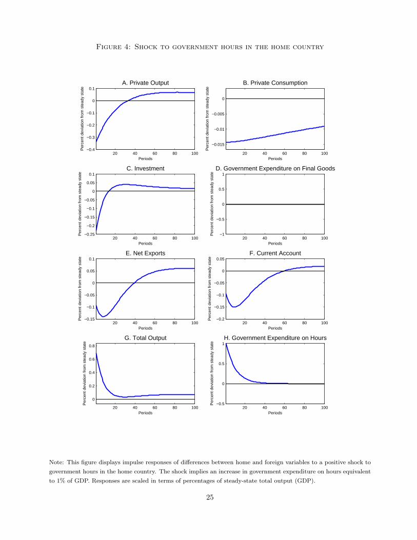
Figure 4: Shock to government hours in the home country

20 40 60 80 100−0.4

−0.3

−0.2

−0.1

0

0.1A. Private Output

Periods

Per

cent

dev

iatio

n fr

om s

tead

y st

ate

20 40 60 80 100

−0.015

−0.01

−0.005

0

B. Private Consumption

Periods

Per

cent

dev

iatio

n fr

om s

tead

y st

ate

20 40 60 80 100−0.25

−0.2

−0.15

−0.1

−0.05

0

0.05

0.1C. Investment

Periods

Per

cent

dev

iatio

n fr

om s

tead

y st

ate

20 40 60 80 100−1

−0.5

0

0.5

1D. Government Expenditure on Final Goods

Periods

Per

cent

dev

iatio

n fr

om s

tead

y st

ate

20 40 60 80 100−0.15

−0.1

−0.05

0

0.05

0.1E. Net Exports

Periods

Per

cent

dev

iatio

n fr

om s

tead

y st

ate

20 40 60 80 100−0.2

−0.15

−0.1

−0.05

0

0.05F. Current Account

Periods

Per

cent

dev

iatio

n fr

om s

tead

y st

ate

20 40 60 80 100

0

0.2

0.4

0.6

0.8

G. Total Output

Periods

Per

cent

dev

iatio

n fr

om s

tead

y st

ate

20 40 60 80 100−0.5

0

0.5

1H. Government Expenditure on Hours

Periods

Per

cent

dev

iatio

n fr

om s

tead

y st

ate

Note: This figure displays impulse responses of differences between home and foreign variables to a positive shock to

government hours in the home country. The shock implies an increase in government expenditure on hours equivalent

to 1% of GDP. Responses are scaled in terms of percentages of steady-state total output (GDP).

25

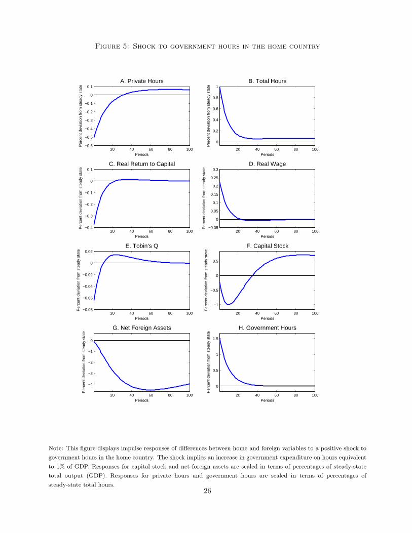
Figure 5: Shock to government hours in the home country

20 40 60 80 100−0.6

−0.5

−0.4

−0.3

−0.2

−0.1

0

0.1A. Private Hours

Periods

Per

cent

dev

iatio

n fr

om s

tead

y st

ate

20 40 60 80 100

0

0.2

0.4

0.6

0.8

1B. Total Hours

Periods

Per

cent

dev

iatio

n fr

om s

tead

y st

ate

20 40 60 80 100−0.4

−0.3

−0.2

−0.1

0

0.1C. Real Return to Capital

Periods

Per

cent

dev

iatio

n fr

om s

tead

y st

ate

20 40 60 80 100−0.05

0

0.05

0.1

0.15

0.2

0.25

0.3D. Real Wage

Periods

Per

cent

dev

iatio

n fr

om s

tead

y st

ate

20 40 60 80 100−0.08

−0.06

−0.04

−0.02

0

0.02E. Tobin‘s Q

Periods

Per

cent

dev

iatio

n fr

om s

tead

y st

ate

20 40 60 80 100

−1

−0.5

0

0.5

F. Capital Stock

Periods

Per

cent

dev

iatio

n fr

om s

tead

y st

ate

20 40 60 80 100

−4

−3

−2

−1

0

G. Net Foreign Assets

Periods

Per

cent

dev

iatio

n fr

om s

tead

y st

ate

20 40 60 80 100

0

0.5

1

1.5

H. Government Hours

Periods

Per

cent

dev

iatio

n fr

om s

tead

y st

ate

Note: This figure displays impulse responses of differences between home and foreign variables to a positive shock to

government hours in the home country. The shock implies an increase in government expenditure on hours equivalent

to 1% of GDP. Responses for capital stock and net foreign assets are scaled in terms of percentages of steady-state

total output (GDP). Responses for private hours and government hours are scaled in terms of percentages of

steady-state total hours.26