global income inequality - world...
TRANSCRIPT

What do we know about global income inequality?
Sudhir Anand
Department of Economics, University of Oxford
and St Catherine’s College, Oxford
Paul Segal
Nuffield College, Oxford
Draft, October 2006

1
What do we know about global income inequality?
Sudhir Anand and Paul Segal
1. Introduction
The last few years have seen a spate of papers estimating global income inequality. Their
appearance is in part motivated by a desire to understand the effects of ‘globalization’,
and has been made possible by recent increases in the availability of data on income
distributions within countries. Controversy centres on whether inequality has increased
or decreased in the recent past. The direction and magnitude of change have been highly
charged questions with some authors arguing that globalization has benefited the rich
disproportionately, while others argue that it has reduced world income inequalities.
Various findings are cited in the media, including the financial press, typically to support
one or another position on globalization.
In this paper we will review the literature on global interpersonal inequality, including the
studies by Bhalla (2002), Bourguignon and Morrisson (2002), Chotikapanich, Valenzuela
and Rao (1997), Dowrick and Akmal (2005), Dikhanov and Ward (2002), Korzeniewicz
and Moran (1997), Milanovic (2002, 2005), Sala-i-Martin (2006), and Schultz (1998).
These studies cover different time periods up to the 1990s or later (1989 in the case of

2
Schulz 1998), use different methods of estimation, and rely on different datasets. They
all estimate the level of and change in global interpersonal income or consumption
inequality, using a variety of inequality measures. Earlier papers have also estimated
global inequality, such as Berry, Bourguignon and Morrisson (1983) and Grosh and
Nafziger (1986), but they were based on very limited income distribution data and in this
regard the literature has advanced considerably.1 Several other papers look solely at
trends in within-country inequality around the world. For example, Cornia and Kiiski
(2001) examine changes in income and consumption inequality within countries, and
Galbraith et al. (1999) measure the evolution of industrial earnings inequality. Yet other
studies, such as Firebaugh (1999, 2003) and Boltho and Toniolo (1999), estimate
between-country inequality only, while Melchior et al. (2000) estimate between-country
inequality and report trends in regional Gini coefficients. However, none of these studies
constructs a measure of global inequality which takes account of both between- and
within-country inequality, and are therefore outside the scope of this review.
The changes in inequality found in these studies have often been adduced as evidence for
or against the benefits of increased international economic integration. Quite apart from
the problem of attributing causality,2 we contend that the measured changes do not
appear to be statistically significant on the basis of the standard errors estimated in some
of the studies. Some changes, such as in Milanovic (2002), appear large for the time
1 Berry et al. (1983: 219) use data from “the developed countries and about forty less developed countries”, stating that “[F]or many L.D.C.s data at the national level is either non-existent or extremely weak.” Even as late as 1992 income distribution estimates were available for only 41 out of 185 countries listed in the World Bank’s (1992) World Development Report. 2 For example, much of the increase in incomes of the poor in China occurred as a result of changes in government policy on domestic foodgrain prices in the early 1980s and mid 1990s, and had little if anything to do with increased international economic integration (Riskin 2006).

3
period over which they are measured, but they are nonetheless small relative to plausible
standard errors. Other sources of uncertainty (e.g. measurement and estimation
problems) that are not incorporated in the estimated standard errors would lead to even
wider confidence intervals. Such uncertainty, combined with the disagreement among
the studies, leads us to the view that we cannot tell whether global inequality has
increased or decreased in the recent past on the basis of existing findings.
The paper proceeds as follows. Section 2 begins by asking what kind of global inequality
we want to measure, and why. In section 3 we present an overview of the studies.
Section 4 discusses each study in turn and critically reviews the data and methodology
used. Section 5 discusses the decomposition of global inequality into between-country
and within-country components, and the significance of China and India. In section 6 we
discuss methodological and data questions, including the use of purchasing power parity
(PPP) versus market exchange rates, measurement error, and the role of national accounts
data. Section 7 is in conclusion.
2. What do we want to measure and why?
There are many reasons to be interested in global inequality. Three angles of interest,
ranging from the moral to the explanatory, can be readily identified. First, we may be
interested in global inequality intrinsically, as large disparities in individuals’ incomes
may be considered unjust. Secondly, we may be interested in global inequality as an
explanation for, or predictor of, some phenomenon of interest. Thus, unequal voting or
bargaining power in international institutions may be a reflection of income inequalities

4
among countries; or migration may be partly determined by global income inequalities as
relatively poor people migrate to raise their living standards. Finally, we may be
interested in global inequality as a predicted outcome of a theory, such as the
convergence in per capita incomes across countries predicted by neoclassical growth
theory, or the divergence predicted by dependency theory.
The appropriate definition of ‘global inequality’ depends on the purpose at hand.
Milanovic (2005) provides a useful distinction between three concepts of world income
inequality. Concept one is inequality among countries in their levels of average per
capita income, with each country counting as a unit. Concept two is what we refer to as
between-country inequality, which is inequality among individuals in the world with each
individual assigned the average per capita income of his or her country of residence.
Concept three is global interpersonal inequality, or global inequality for short, which is
inequality among individuals in the world with each individual assigned his or her own
(per capita household) income. Concept two can readily be seen as the same as the
‘between-country component’ of global inequality. It measures what global inequality
would be if incomes were to be equally distributed among individuals within each
country. Finally, to Milanovic’s three concepts we would add a ‘concept zero
inequality’, which refers to inequality among countries ranked by total (not per capita)
income. The population unit of concepts zero and one is the country, while that of
concepts two and three is the individual.3 In all cases it remains to choose an appropriate
‘income’ concept, e.g. consumption expenditure or income, assigned to the population
3 Concepts two and three inequality could in principle also be defined across households rather than individuals.

5
unit in question (country or individual). This is important because, for instance, concept
three inequality applied to income could move in a different direction from concept three
inequality applied to consumption expenditure. This issue is discussed later.
To measure global inequality we must also choose a set of exchange rates with which to
convert national currencies into a common numeraire. The options are, broadly speaking,
market exchange rates (say, relative to the US dollar) versus purchasing power parity
(PPP) exchange rates.4 PPP exchange rates take into account price differences across
countries. They allow for the fact that a dollar’s worth of rupees, bought on the currency
markets, will buy more of most goods and services in India than the same dollar would
buy in the US. For developing countries, incomes measured using PPP exchange rates
can be three or four times higher than when measured at market exchange rates.
Wade (2001) suggests that market exchange rates are more appropriate than PPP
exchange rates “for most of the issues that concern the world at large”, including
“migration flows” and “the extent of marginalization of developing countries in the world
polity; and, more broadly, the economic and geopolitical impact of a country (or region)
on the rest of the world”. It seems more plausible to us that relative incomes measured at
PPP exchange rates would be the better predictor of migration flows. Remittances sent
by migrants are indeed exchanged into national currencies on the market, but to the extent
that people migrate to raise their own standard of living, it is PPP exchange rates that
matter. On the other hand, market exchange rates do seem to be more appropriate in
4 The two options are broad in the sense that choices remain within each: there will be different methods of smoothing market exchange rates over the year, and there are different methods for calculating PPP exchange rates. We consider PPP exchange rates in more detail later in the paper.

6
measuring “the economic and geopolitical impact of a country (or region) on the rest of
the world”. In this case the variable of interest is presumably total income, not per capita
income. This is one of the factors that underlies China’s significance in world politics,
and makes India and Brazil important in international trade negotiations. The appropriate
inequality concept here would seem to be concept zero inequality, or gross national
income across countries measured at market exchange rates.
Other questions call for different combinations of inequality concept and exchange rate.
Consider the question of convergence between countries. This is based on concept one
inequality where the country is the population unit, assigned its level of per capita
income. As the variable of interest is the level of output per head, it is natural to use PPP
exchange rates (e.g. Pritchett 1997).
These questions are not our concern in this paper. The studies reviewed here are
concerned with global inequality from two points of view. First, it is of interest
intrinsically, as a measure of the distribution of goods or resources among individuals in
the world. Within countries, high levels of inequality are often taken to indicate a lack of
fairness in society and governments act to reduce inequality – for example, through
progressive tax-benefit policies. At the global level there are some redistributive
mechanisms, e.g. foreign aid. Moreover, rules governing economic interactions between
rich and poor countries, e.g. intellectual property rights over pharmaceuticals, will affect
global inequality. A concern for “global justice” will lead to an interest in concept three
inequality.

7
Secondly, changes in global inequality are sometimes portrayed as consequences of
‘globalization’. As trade and financial flows among countries increase, mediated by
governments and international institutions that substantially influence the terms of these
exchanges, questions of distribution across countries immediately arise. Thus the
evolution of global inequality may tell us something about globalization. Although
several of the studies reviewed here attribute changes in global inequality to
globalization, none presents any causal analysis. Nonetheless, measuring trends in global
inequality would be an important preliminary for such an analysis.
Since our main concern is inequality of real income (or consumption) among individuals,
it is natural to use PPP exchange rates. However, from a technical point of view the
difference between inequality as measured at PPP rates and at market exchange rates is
itself of interest. The divergence reported by studies between trends in inequality at
different exchange rates may imply something about economic structure, which we
discuss later. Thus we also report global interpersonal inequality at market exchange
rates.
We have so far said nothing of concept two inequality, which assigns to each individual
in the world the per capita income of his or her country. As the between-country
component in the decomposition of concept three inequality, it is useful for explaining
the sources of global interpersonal inequality and its changes over time. In addition,

8
some studies (e.g. Firebaugh 1999, 2003) have used it as a downward-biased estimator
for concept three inequality.
3. An overview of global inequality
As a first cut at estimating international inequality, UNDP (1999) and World Bank (2000)
report changes in the ratio of per capita GDP of the richest countries to that of the poorest
countries. This is a measure of concept one inequality as it takes the country as the unit
of analysis and per capita GDP (at PPP exchange rates) as the income concept. World
Bank (2000: 51) reports that in 1960 the per capita GDP of the 20 richest countries was
18 times that of the 20 poorest countries, while in 1995 the ratio had grown to 37. UNDP
(1999: 38) notes that the ratio of the per capita GDP of the richest country to that of the
poorest country grew from 35 in 1950, to 44 in 1973, and 72 in 1992.5 Like Pritchett’s
well-known (1997) analysis, this represents “divergence, big time”.
Matters are not so simple, however, when we turn to concept three global interpersonal
inequality. All studies agree that the level is very high: for example, estimates of the Gini
coefficient using standard purchasing power parity income (sourced from the World
Bank, Maddison, or the Penn World Tables) in the 1990s lie within the range of 0.609 to
5 Both Bhalla (2002) and Australian Treasury (2001) object to this procedure, claiming that because it uses different countries in the two years of comparison, the measure is biased. They claim that the correct procedure would be to compare the relative incomes of the same groups of countries in the two years, and that this results in a decline in inequality. Bhalla (2002: 24) states that the income ratio between the richest 20 and poorest 20 countries in 1960 is 23, and that the ratio between these same two groups of countries falls to 9.5 in 2000. This criticism is mistaken. It is an axiom of inequality measures that they are ‘anonymous’, i.e. they do not distinguish between individuals (countries) other than by their income levels. That is, inequality measures are functions of the vector of incomes, which are invariant to permutations of the vector, i.e. they are independent of the individual (or country) names attaching to the incomes. The World Bank and UNDP methodology satisfy this axiom, while Bhalla’s does not.

9
0.686. These levels are comparable to those found within the most unequal countries,
such as Namibia and Botswana, with Ginis of 0.707 and 0.630 respectively, according to
World Bank (2002).
In contrast, no consensus emerges concerning the direction of change in global inequality
in the last twenty to thirty years. For example, Dowrick and Akmal (2005) find that the
Gini falls from 0.659 in 1980 to 0.636 in 1993 when using standard PPP conversion
factors, but that it rises slightly from 0.698 to 0.711 using their own ‘Afriat’ PPP
conversion factors (on which more below). Sala-i-Martin (2006) finds it to decrease from
0.660 in 1980 to 0.637 in 2000, and Bhalla (2002) records a reduction from 0.686 in
19806 to 0.651 in 2000. In contrast, Bourguignon and Morrisson (2002) find no change
in the Gini between 1980 and 1992, which remains at 0.657, while their estimate of the
Theil T index increases from 0.829 to 0.855. Milanovic (2005) finds that the Gini
coefficient increases from 0.622 to 0.641 between 1988 and 1998.
Several studies estimate what they call the ‘Theil’ measure of inequality. Unfortunately,
the authors are not referring to the same (Theil) inequality index. In Chotikanapich et al.
(1997), Milanovic (2002, 2005), and Dikhanov and Ward (2002),7 the ‘Theil index’
refers to the Theil L measure or the mean logarithmic deviation (Anand 1983: 89-91), but
in Bourguignon and Morrisson (2002), Dowrick and Akmal (2005), Korzeniewicz and
6 This information can be roughly read off the graph in figure 11.1 of Bhalla (2002). This number is also given in Table 5.2 on p. 80 of the third draft of Bhalla (2002), circulated in December 2001, but the table and this number do not appear in the final published version. 7 In discussing the ‘Theil’ index, Dikhanov and Ward provide the formula for the Theil L measure. They also estimate what they call the ‘Theil 2’ index but do not provide any formula for it. We assume it refers to the Theil T index.

10
Moran (1997), and Sala-i-Martin (2006, 2002a, b), the Theil index refers to the Theil T
entropy measure.8
Estimated changes in the Theil indices are typically larger in proportional terms than
those in the Gini. Given that both Theil indices are more sensitive than the Gini to
changes at the extremes of the distribution, one explanation might be that changes in the
incomes of the richest relative to those of the poorest have been more significant than
those in the middle of the distribution. The findings in Milanovic (2002) that the ratio of
the income of the richest 5% to the poorest 5% increased from 78 in 1988 to 114 in 1993,
and in Bourguignon and Morrisson (2002) of an increase in the global income share of
the top 5% between 1980 and 1992, are consistent with this explanation.
Four of the studies also calculate global inequality at market exchange rates. The level
found is, not surprisingly, substantially higher than when PPP incomes are used, and all
four studies also report an increase over time. Dowrick and Akmal find that the Gini
rises from 0.779 to 0.824 between 1980 and 1993, Milanovic (2002) from 0.782 to 0.805
between 1988 and 1993, Korzeniewicz and Moran from 0.749 to 0.796 between 1965 and
1992, and Milanovic (2005) from 0.778 to 0.794 between 1988 and 1998.
With increasing globalization one would expect market exchange rates to move closer to
PPP exchange rates (as countries trade larger proportions of their GDP). The apparent
divergence over time between inequality measured at market and at PPP exchange rates
8 Milanovic (2002) does not specify which Theil index he uses, so we contacted the author directly for this information.

11
thus requires some explanation. Dowrick and Akmal (2005) attempt to address this
question (discussed below), but in our view the relationship between changes in global
inequality at PPP and at market exchange rates merits further research.
4. The studies
The studies reviewed here make use of a variety of methods, measurements and datasets.
In this section we describe the findings and distinguishing features of each study, and
comment on their calculations. Table 1 and Figures 1 and 2 summarize their results;
Table 2 summarizes their sources. Issues that arise in relation to several or all of the
papers are discussed in Sections 5 and 6.
Milanovic (2002, 2005)
Milanovic (2002) uses income or expenditure taken directly from national household
surveys to construct a ‘true’, in the sense of directly observed, world distribution of
income/consumption. Using PPP exchange rates for consumption, from both the Penn
World Tables (PWT) and the World Bank, he finds that inequality increases over the
five-year period 1988-1993 (see our Table 1). Moreover, the 1988 distribution Lorenz-
dominates the 1993 distribution, and hence will show less inequality for all measures in
the Lorenz class of indices (Anand 1983: 339-40). His later book, Milanovic (2005),
updates the estimates to 1998. He finds that inequality falls over 1993-98, but remains
some two Gini points higher in 1998 than in 1988 (see our Table 1).

12
Milanovic’s (2002) data comprise a total of 216 country surveys benchmarked to the two
years 1988 and 1993, which are obtained from the World Bank and other sources.9
Milanovic’s (2005) study, which includes the benchmark year 1998, has a sample of 345
country surveys. Unlike every other study, Milanovic constructs inequality estimates
over time for a common sample of countries. The common sample is slightly different in
the two studies but in both cases covers about 84% of the world’s population. Most of
his within-country distributions are described by at least ten quantile shares or income
groups, and he assumes that each individual or household within a group has the same
income.
Milanovic’s estimates raise a number of questions. First, countries in the common
sample have different numbers of income groups in the different benchmark years, with
the average number of data points (income groups) per country-year standing at 10.8 in
1988, 11.4 in 1993, and 15.1 in 1998. Hence the under-estimation due to the assumption
of equal incomes within income groups would be expected to be different in each year.
Secondly, the measured distribution within China is of concern. Milanovic (2002) has
several income groups in rural China each containing more than 100 million people, with
the largest containing 180 million in 1993 (and 175 million in 1990 for the benchmark
9 The sample that is common to both 1988 and 1993 consists of 91 countries; in addition, for 1988 he has data for another 10 countries, and for 1993 for another 28 countries. Thus the total number of countries in 1988 is 101 and in 1993 it is 119. The total of 220 country-years is larger than the 216 country surveys. This may be due to his splitting of four large countries (China, India, Bangladesh and Indonesia) into urban and rural areas in both years and treating them as different countries. He similarly splits Pakistan in 1988 but not in 1993. However, even when we count these observations as distinct surveys for different country-years we are unable to make the numbers tally.

13
year 1988).10 The presence of such large groups could lead to possibly-substantial
downward biases in measured inequality.
Thirdly, to achieve finer-grained distributions Milanovic (2002: 60) states that he splits
four large countries in 1993 and five in 1988, including China and India, into rural and
urban areas (for which he has separate distributions) and treats these observations as
different ‘countries’.11 However, in two of these countries – Bangladesh12 and Indonesia
– the corresponding urban and rural income groups have near-identical mean incomes for
all but the top and bottom income groups (presumably because the same absolute income
intervals were used to code urban and rural incomes). Hence, even though the urban and
rural population shares in each income group are different, the urban-rural disaggregation
adds almost no information.13 Note that this is not the case for India and China, where it
would really matter: their income groups have different mean incomes in rural and urban
areas.
Milanovic (2002: 61) also reports using different PPP rates for rural and urban China to
take account of price differences between the strata: “For China, in 1993, I use the rate
reported in the International Comparison Programme (ICP) for urban areas only (since
10 This largest group is equal in size to the combined populations of the 50 smallest countries in his dataset, which between them have more than 500 income groups. 11 This implies that his ‘between-country’ component of global inequality actually includes some within-country inequality. 12 In his on-line (2002) dataset we could find Bangladesh split into urban and rural areas only in 1988, not 1993. 13 In his dataset the income distribution for Egypt in 1988 is also shown separately by urban and rural areas, with five income groups in each area. The income groups are shown as quantiles (bottom two quintiles, middle 40%, and top two deciles) for each sector. Surprisingly, the second-to-top decile for the urban and rural sectors have identical mean incomes, and for all quantiles other than the bottom quintile the urban and rural mean incomes are very close. Effectively this means he only has five or six income groups for Egypt, not ten.

14
the rate itself was obtained from surveys conducted in two cities: Guangdong and
Shanghai), and reduce the price level in rural areas by an estimated 20% (see Yao and
Zhu 1998, p. 138)”. Yao and Zhu (1998: 138) themselves suggest adjusting rural
incomes upwards relative to urban incomes by “15 per cent for low cost of living in the
countryside”. This is equivalent to adjusting rural prices relative to urban prices down by
13%, not 20%.
Bourguignon and Morrisson (2002)
Bourguignon and Morrisson (2002) estimate global inequality back to the 19th century,
starting in 1820 and ending in 1992. They assemble data for 33 countries or groups of
countries, where 15 countries with large populations or economies (such as China, India,
Italy and the US) are considered individually, and all other countries are clustered into 18
country groups. For each country or country group they combine data on GDP per capita
in PPP$ with income shares for 11 quantiles – the bottom nine deciles and the top two
vigintiles (5% of population).14 Thus their estimates of global inequality for each year
are based on 363 (33x11) data points. Like Milanovic, they assume incomes to be
equally distributed within each quantile. Unlike Milanovic, who takes incomes or
expenditures directly from household surveys, they scale within-country distributions to
per capita GDP, recognizing that “[b]ecause of the obvious discrepancy between
household purchasing power and GDP per capita, using GDP per capita in place of mean
14 They use per capita GDP data from Maddison (1995) and describe filling in gaps in GDP and population data by applying “growth rates observed for comparable neighbouring countries over the same period” (Bourguignon and Morrisson 2002: 729). Income distribution data are obtained from a variety of sources. For countries without data, the “distribution was arbitrarily assumed to be the same as in a similar country for which some evidence was available for the appropriate period” (Ibid.: 730).

15
personal income may bias the estimation of the evolution of world inequality. Correcting
for the share of non-household income in GDP or the share of non-consumption
expenditures or taking into account the effects of changes in the terms of trade on the
purchasing power of national agents proved impossible for the historical period. For
comparability reasons, the GDP per capita convention was retained even after 1950,
though a better approximation of international differences in mean living standards would
have been possible” (Ibid.: 730).
They find that inequality increases between 1820 and 1950, according to all measures,
and that the subsequent trend varies by inequality measure (see our Table 1). All indices
except the standard deviation of log-income are higher in 1992 than in 1970. The income
shares of the top quintile, decile and vigintile increased uniformly from 1970 to 1992, the
top decile increasing its share from 50.8% in 1970 to 53.4% in 1992. The share of the
bottom 20% was the same in 1992 (2.2%) as in 1970, with a slight trough in 1980 (2.0%).
They decompose the Theil T and the mean log deviation (MLD) into between- and
within-‘country group’ components, but their use of 33 country groups rather than
individual countries to decompose inequality makes their decompositions not comparable
with those in other studies.

16
Sala-i-Martin (2006)
Sala-i-Martin (2006) estimates global income distributions using within-country quintile
shares scaled to per capita GDP in PPP$.15 He uses quintile share data from Deininger
and Squire (1996 updated), extended with UNU-WIDER data, and takes per capita GDP
in PPP$ from the Penn World Tables 6.0 (Heston, Summers and Aten 2002, and known
as PWT). He presents estimates for global inequality for each year between 1970 and
2000 based on observed and estimated data for 138 countries, representing 93% of the
world’s population in 2000. For those countries with survey data for more than one year,
representing 84% of the world’s population, he uses “a simple linear time-trend forecast”
(p. 358) to fill in quintile shares for missing years. For countries with data for only one
year he assumes a linear trend based on an average for “neighboring countries” (p. 359),
defined as those belonging to the same World Bank region, which have surveys for more
than one year. For countries with no survey data, he imputes average quintile shares and
estimated trends from neighbouring countries.
With these quintile shares Sala-i-Martin estimates for each country-year a smoothed
density function using a Gaussian kernel with the same bandwidth in every case. Each
kernel density function is normalized by population size and scaled to per capita GDP
from PWT. These within-country distributions are aggregated to construct a world
income distribution.16 For every measure he finds inequality to be higher in 1980 than in
15 This paper follows two previously-circulated working papers (Sala-i-Martin 2002a, b). 16 Sala-i-Martin (2002b) uses the same procedure to estimate a world income distribution, while in Sala-i-Martin (2002a) he arrays the quintile data points for 125 countries to form a ‘spiked’ world distribution which is then smoothed by means of a Gaussian kernel density function.

17
1970, but lower in 2000 than in 1980 (see our Table 1). For the variance of log-income
inequality is higher in 2000 than in 1970, but for other measures it is lower.
Sala-i-Martin defends his use of per capita GDP as the mean for within-country
distributions, instead of using mean incomes from surveys, by observing that surveys are
available for only few years. He objects that “we would have to somehow forecast these
survey means for the missing country/year cells” (p. 357). But missing values for
quintile shares for most years did not deter him from ‘forecasting’ within-country
distributions. More importantly, as Bourguignon and Morrisson (2002: 730) point out,
GDP per capita has obvious failings as a measure of household income. We discuss the
question of scaling within-country distributions to national accounts categories later in
Section 6. For now, note that while the national accounts category of household
consumption expenditure is different from household income, GDP is also different from
household income as it includes several components of non-household income.17
Sala-i-Martin (2006: Table IV, p. 390) reports the within- and between-country
components for the MLD and the Theil T index. For both measures between-country
inequality comprises about 70% of global inequality in 1970, falling to just over 60% in
2000. This is due to an absolute rise in within-country inequality and an absolute decline
in the between-country component. Sala-i-Martin’s (2006: 388) definition of the “within-
country” component is “the amount of inequality that would exist in the world if all
countries had the same income per capita (that is, the same distribution mean) but the
17 Sala-i-Martin (2006: 357, fn 5) cites Deaton (2005) in describing some of the disadvantages of using household consumption from national accounts. However, Deaton’s point is that these are disadvantages relative to the use of survey means, and not relative to GDP.

18
actual within-country differences across individuals” (see also his note to Table IV, p.
391). While this is correct for the within-country component of the MLD measure, it is
not correct for that of the Theil T index, both of which are presented in his Table IV. We
discuss this further in Section 5 below.
In addition to presenting his own analysis of global income inequality, Sala-i-Martin
(2006: 382) comments on the discussion of the subject in the 2001 Human Development
Report (HDR) of the United Nations Development Programme (UNDP 2001). He writes
that it “argues that global income inequality has risen based on the following logic:
Claim 1: ‘Income inequalities within countries have increased.’
Claim 2: ‘Income inequalities across countries have increased.’
Conclusion: ‘Global income inequalities have also increased.’”
Sala-i-Martin points out that if Claim 2 refers to what we described as concept one
inequality, which counts each country as a unit, then the conclusion does not follow,
stating that “[B]y adding up two different concepts of inequality to somehow analyze the
evolution of world income inequality, the UNDP falls into the fallacy of comparing
apples to oranges” (p. 382). However, UNDP (2001) does not make this argument, and
makes no reference to changes in global interpersonal inequality.18
18 It states that “World inequality is very high” (UNDP 2001: 19). Sala-i-Martin (2006: 382, fn. 26) also refers to HDR 2003, but that publication states that trends in global income inequality are “ambiguous” (UNDP 2003: 39), not that they are rising.

19
Bhalla (2002)
Bhalla (2002) constructs annual estimates of global inequality for income and
consumption separately for each year during 1950-2000. He finds that the global income
Gini increases from the late 1950s to the early 1970s (late 1970s for consumption), and
then decreases until 2000 (2002: Fig. 11.1, p. 174).
Bhalla scales within-country distributions to per capita GDP for his measurement of
global income inequality,19 and to household final consumption expenditure (HFCE)
from national accounts (NA) for consumption inequality,20 both measured at PPP (the
sources of which are unclear—see below). According to his Figure 11.1 on p. 174, his
sources for within-country inequality are Deininger and Squire (1996); World Income
Inequality Database (WIID, available at www.wider.unu.edu/wiid); World Bank, World
Development Indicators, CD-ROM; Asian Development Bank (2002).21 There is some
confusion regarding the number of surveys he uses to construct his global inequality
estimates. Table A.1 on p. 209 records that there are 317 surveys (income and
expenditure) for the period 1950-1980, and 604 for the period 1980-2000, for a total for
921. But in the text he writes that “Construction of the dataset required the use of data
for more than 1,000 household surveys” (2002: 38). Whatever the precise number may
19 This is nowhere stated explicitly, as far as we can tell, but we deduce it from his comments that “published national accounts figures, provided the best basis for estimating world inequality” (2002: 173) and that “household income has to be approximated by per capita GDP” (Ibid.: 103-4, footnote 1). 20 In fact, consumption distributions are constructed by scaling within-country distributions to 0.867 times HFCE from NA (2002: 128), but since this scaling is uniform across the world it makes no difference to his estimates of inequality (the deflation is for the purpose of estimating absolute income poverty). 21 Yet on pp.212-3 he refers only to the first three and to the World Development Indicators website. Still elsewhere, on p. 208, he mentions that the Deininger and Squire (1996) and WIID datasets “have been supplemented by data available from the Web (World Bank poverty monitor, worldbank.org/research/povmonitor; and Milanovic’s data on Eastern European countries), as well as data gathered for 18 Asian countries (Asian Development Bank 2002)”. From such documentation it is unclear exactly which sources have been used by Bhalla to provide his within-country distributions.

20
be, he has to impute within-country distributions for the majority of his 7,599 country-
years (149 countries times 51 years). Moreover, there is concern regarding the quality of
the surveys that he uses. Ravallion (2002: 8) observes that only “[a]bout half of Bhalla’s
600 distributions over 1980-2000 would pass the quality standards applied to the [World]
Bank’s calculations”.
Like Sala-i-Martin (2006) Bhalla uses the quintile share data to estimate continuous
within-country distributions, employing what he calls the “simple accounting procedure
(SAP)” (2002: 6). Whereas Sala-i-Martin (2006) uses non-parametric density estimation,
Bhalla uses regression to fit a three-parameter Lorenz curve to the quintile shares
(comprising four independent observations, since they add up to 1), using a functional
form due to Kakwani (1980). However, he does not stop here. He states that “The basic
equation results are then filtered by SAP to satisfy the theoretical boundary constraints
(i.e., the sum of the estimated shares of each quintile is actually equal to the observed
shares, and the share of each percentile is equal to or larger than the share of the previous
percentile). The filtering is done through an iterative procedure, whereby at the end of
the first round, the shares of each individual percentile in the first quintile get estimated
and fixed, then the next quintile, then the next, and so on. (The only somewhat
“arbitrary” and somewhat “flexible” percentiles are the first and the last, and this
flexibility shows up in the errors; see below.)” (pp. 133-4, emphasis in original). We are
unable to decipher exactly what the procedure entails.22 If his object is to force the
estimated Lorenz curve through the four observed cumulative quintile shares, then there
22 This procedure is described even more opaquely in Appendix B, p. 212.

21
are many ways to achieve this while satisfying his constraint that the curve be convex.23
Moreover, it is not clear what role the initial fitted Lorenz curve is playing in this
procedure. Given the inadequate documentation it is impossible to replicate his results
independently, violating the first criterion for empirical research.
Bhalla reports accuracy tests of his estimation method against unit-level data from India
and against published data on “selected percentiles, and the Gini” for the US. For India
he claims that “The SAP method is seen to be shockingly accurate. The constructed
Ginis are within 1 percent of the true value in almost 90 percent of the cases” (2002:
214). For the US he claims “[T]he constructed and original Ginis are within a whisker of
each other for all the years” (Ibid.: 134). He concludes that “[t]he tests above suggest
that the SAP method is accurate both at the aggregate Gini level (very, very accurate) and
at the individual percentile level (very accurate)” (Ibid.: 134). Without knowing how the
SAP method works it is not possible for us to comment on these tests. For all the reader
can tell, the method could have been constructed in order to fit the US and Indian data,
implying that its accuracy in these cases tells us nothing about its potential accuracy in
other cases. Ravallion (2002: 14-5) writes “[T]he fact that one specific Lorenz curve
model gives a good fit for one country does not mean it will fit well for others. Indeed,
we find that very different models of the distribution (either Lorenz curves or density
estimation) are needed in different countries, and even different dates for the same
country”.
23 That is, “the share of each percentile is equal to or larger than the share of the previous percentile”.

22
After estimating within-country distributions, Bhalla scales these to per capita GDP and
per capita HFCE measured in PPP$. His use of PPP sources is problematic. On p. 207
he reports using “Penn World Tables, 1985-base PPP prices, referred to as PWT 5.6; WDI
1998, which has PPP data, 1987 base, at both constant and current prices; PPP data, 1975
base, from Summers and Heston (1988), Heston and Summers (1991), referred to as HS;
and IMF, International Financial Statistics CD-ROM, 2002” in addition to WDI (edition
not specified) and Maddison (2001). These sources are inconsistent for two reasons.
First, the sources use different methods for calculating PPP rates. For instance, recent
World Bank estimates in the WDI follow the EKS method (Ahmad 2003), while PWT
uses the GK method. These methods are quite different, as we discuss in Section 5.
Secondly, PPPs estimated for different base years are also inconsistent. PPPs are
estimated in the International Comparison Programme (ICP) in a given year t. To
calculate GDP in PPP$ in year t+n one has to scale GDP in year t up or down by the
country’s real growth rate (nominal growth minus a price deflator).24 GDP in PPP$ in
year t+n calculated in this manner can be very different from that obtained by use of an
ICP conducted in year t+n.25,26 Without more information on which source is used for
which countries in which years it is impossible to infer the bias caused by Bhalla’s
confounding of sources.
24 In the case of PWT there is a further stage of reconciliation after this updating. 25 When a country has more than one ICP survey some sort of reconciliation procedure must be used; see Section 5 below. 26 Bhalla laments (2002: 96) that the World Bank’s consumption PPPs—that is, PPP rates based on the consumption component of GDP—are available only for 1993, in contrast to their GDP PPP rates that are available for many years. But, as just described, GDP PPP rates are constructed by measuring relative prices in one year only, and then scaling up and down across years using domestic price deflators. He could therefore have followed the same procedure using 1993 consumption PPPs to construct consumption PPPs for other years.

23
Despite these and other questions that arise in relation to calculations of PPP exchange
rates (see our Section 6), Bhalla seems to disregard any controversy concerning PPP
estimates. He writes: “No one—not the official source of poverty figures, or any
institution, or any outside researcher—is questioning the PPP estimates. This is not
because everyone believes that these figures are accurate; it is only because no one has
the capacity, or the resources, to come up with a ‘better’ estimate of the PPP exchange
rate” (2002: 94). Yet Reddy and Pogge (2005) question the PPP estimates, and Dowrick
and Akmal (2005) present an alternative PPP exchange rate (discussed in our Section 5).
Earlier versions of both papers are cited in Bhalla’s references.
In assessing the accuracy of his Simple Accounting Procedure, Bhalla comments: “Is
there a particular bias in the SAP method? There cannot be, because, as the name
suggests, the procedure is one of simple counting, and simple accounting” (Ibid.: 181-2).
The simplicity of the method will certainly elude the reader, as will the sense in which his
global inequality calculations involve mere “accounting”. Moreover, the lack of
transparency regarding the method and sources preclude the possibility of judging the
extent of bias. Finally, it should be noted that even simple procedures can be biased.
Dowrick and Akmal (2005)
This study follows the approach of Bourguignon and Morrisson (2002) and Sala-i-Martin
(2002a) in pooling within-country quantiles, in this case quintile shares from Deininger

24
and Squire (1996),27 scaled up to GDP per capita. When country GDP is measured using
the standard Geary-Khamis (GK) PPP rates in PWT, they find that all the measures they
estimate (Gini, Theil T, squared coefficient of variation, variance of log-income) decrease
from 1980 to 1993 (see our Table 1). What is novel in their paper is the use of an
alternative PPP exchange rate based on Afriat (1984), which they argue gives a better
measure of comparative purchasing power across countries. When country GDP is
measured using Afriat PPP rates, inequality increases by all measures over the period
1980-1993. They also estimate global inequality at market exchange rates, which they
find to be both considerably higher than when measured at either PPP rate, and to
increase faster than the increase at Afriat PPPs.
They argue that inequality measured at market exchange rates suffers from a “traded
sector bias” and inequality measured at PWT PPPs suffers from a “substitution bias”.
Traded sector bias refers to the fact that exchange rates are affected by the prices of
traded goods across countries but do not reflect domestic prices of non-traded goods.
Since the relative price of non-traded to traded goods tends to be lower in poorer than in
richer countries, valuing domestic incomes at market exchange rates will undervalue
incomes in poorer relative to richer countries and lead to an upward bias in measured
inequality. Substitution bias, also known as the Gerschenkron bias, refers to the fact that
valuing the output of country A at country B’s prices will lead to an overestimation of the
income of country A relative to the income of country B (also valued at B’s prices). In
the case of PWT PPPs the use of the GK method leads to a vector of “international
27 When only Ginis and not quintile share data were available in Deininger and Squire (1996), they estimate the single-parameter functional form for the Lorenz curve suggested by Chotikapanich (1993) and thereby obtain quintile shares.

25
prices” whose structure is closer to that of prices in richer than in poorer countries
(Nuxoll 1994). They state that this leads to the incomes of poorer countries being
overestimated relative to richer countries, and hence to a downward bias in inequality.
Dowrick and Akmal further argue that diverging price structures can explain both the rise
in inequality using market exchange rates and the fall using PWT PPP rates. They
estimate trends in price similarity across countries and find that price structures became
less similar over the period 1980 to 1991 (2005: Fig. 5, p. 213), arguing that this would
cause both traded sector and substitution bias to increase. Inequality at Afriat PPPs does
not suffer from either traded sector or substitution bias, lies between the other two
estimates, and rises only slightly over time. Thus the rise in market exchange rate
inequality and the fall in PWT PPP inequality could both in principle be explained by
increases in the two biases.
We have reservations about the argument regarding traded sector bias. The claim that
this bias increases as “price structures” become less similar assumes that the price
structure in question is the relative price of traded to non-traded goods. However, the
price vector that Dowrick and Akmal use to measure price divergence across countries
comprises the relative prices of private consumption, investment, and government
consumption (2005: 212). These three categories each comprise both traded and non-
traded goods, so their empirical exercise does not establish divergence in relative prices
of traded to non-traded goods across countries. With globalization, moreover, we would
expect the traded sector to expand relative to the non-traded sector, which would

26
contribute to a decline in the bias. The finding of a rise in global inequality at market
exchange rates would thus seem to require further explanation.
Dowrick and Akmal also run simulations based on generated lognormal distributions to
estimate by how much the assumption of equal incomes within quintiles understates
inequality within a country. They find that the variance of log-income for data grouped
by quintiles is 90% of the actual value, while grouping by deciles yields more than 95%
of the actual value (2005: Fig. 8, p. 224). They conclude that “the quintile income shares
that we and other researchers have used are likely to come close to capturing the full
contribution of intra-country inequality to world inequality” (2005: 224). Supposing that
within-country inequality accounts for 35% of global inequality, as measured by varlog,
then a 10% underestimation of within-country inequality in each country would imply a
3.5% underestimation of global inequality. However, Sala-i-Martin estimates global
inequality using pooled quintile shares from his sample of countries in his (2002a) paper,
and smoothed within-country distributions in (2002b), both papers using the same dataset
(which is different from his 2006 dataset). His estimate of the global variance of log-
income in 1998 is 7.7% higher when he uses smoothed within-country distributions.
Moreover, Dowrick and Akmal’s experiment can tell us little about the impact on other
measures of inequality.
Dikhanov and Ward (2002)
This study takes distributions of incomes and expenditures from Milanovic’s (2002)
dataset for “45 of the largest countries…where reasonably consistent distributions were

27
available for more than one reference year” (Dikhanov and Ward 2002: 6). They
estimate smoothed within-country distributions by interpolating third-degree polynomials
between observed points of the cumulative distribution function. They then scale these
within-country distributions to what they refer to as the national accounts category of
“personal consumption expenditure” from World Bank databases, converted into EKS
PPP$. “Finally, a global picture was built up by taking the available income distributions
from the eight largest countries in each ‘continental’ region (for South Asia only five
countries are used as the number of countries in the region is small and the five countries
chosen comprise more than 90% of the total population) and filling the remaining gaps
(about 1/6 in terms of global income and population) according to observed regional
pattern” (Ibid.: 6). They do not explain how they estimate values for missing years. In
particular, they do not explain how they extrapolate backwards to 1970 from Milanovic’s
“benchmark” 1988 data and forwards to 1999 from his “benchmark” 1993 data.
The direction and magnitude of change in inequality depend on the inequality measure
used (see our Table 1). The income share of the bottom decile remains constant at 0.5%
while that of the top decile increases slowly and steadily from 48.5% in 1970 to 54.3% in
1999. Despite the ambiguity in their measures, the authors conclude that “during the last
three decades, the global income distribution became less equal (both between country
and within country)” (Ibid.: 12).

28
Schultz (1998)
Schultz (1998) uses GDP PPP data from the Penn World Tables 5.5, covering 120
countries with 93% of the world population in 1960 and 92% in 1989. He takes quintile
shares for countries from Deininger and Squire (1996), using data only on those countries
for which there are at least two nationally representative samples since 1950. This yields
509 observations across 56 countries. He then runs regressions on these observations
with log per capita GDP, per capita GDP squared, year, and dummies for type of survey
distribution and region in order to estimate within-country inequality for country-years
without data.
He uses the variance of log-income (varlog) as his measure of inequality in order to
construct global interpersonal inequality as the sum of within-country inequality and
between-country inequality. However, there appears to be a problem with his procedure.
The variance of log-income is decomposable into “between-country” and “within-
country” inequality only if “between-country” inequality is calculated by assigning to
everyone within a country the country’s geometric mean income, not its arithmetic mean
income (Anand 1983: 201, 330-1). The “between-country” component thus calculated
can then be added to the population-weighted within-country varlogs to give the global
varlog. However, the “between-country” component calculated by Schultz is based on
the per capita GDP of countries, i.e. their arithmetic mean incomes. He is evidently
aware of this issue and points out that “the national income variable should refer to the
mean of the logarithms of income” rather than “arithmetic mean income that is logged in
this analysis of intercountry income inequality” (endnote 8). However, the problem

29
remains, and the figures that Schultz reports do not refer to the global variance of log-
income.
Chotikapanich, Valenzuela and Rao (1997)
This study estimates lognormal income distributions for countries from Gini coefficients
reported in Deininger and Squire (1996), which are then scaled to per capita GDP in
PPP$ from PWT 5.6. Their sample of Gini coefficients comprises 36 countries, for
which they estimate lognormal distributions for the years 1980, 1985, and 1990.
However, Africa is represented by only Tunisia and Mauritius, comprising 1.5 percent of
that continent’s population. The virtual omission of sub-Saharan Africa, with about 10
percent of the world’s population, is a major problem for their estimates of changes in
global inequality. Since sub-Saharan Africa includes many of the poorest countries in the
world, and the per capita GDP of this region fell by 10 percent over 1980-90 (World
Development Indicators Online), its omission will lead to a downward bias in changes in
measured global inequality.
Korzeniewicz and Moran (1997)
This study estimates global inequality in 1965 and 1992 at market exchange rates only.
Korzeniewicz and Moran estimate global inequality using quintile shares for 46
countries, mostly from World Bank (1994), scaled to per capita GNP at market exchange
rates. They estimate the Gini and Theil T, finding both to have risen (see our Table 1).

30
The income share of the poorest 30 percent declined dramatically from 2.1 to 1.0 percent,
while the top 20 percent enjoyed a rise in their share from 82.0 to 88.9 percent.
5. Decomposing global inequality
Inequality between and within countries
Many studies that estimate global income inequality “decompose” overall world
inequality into between- and within-country components. Thus, Milanovic (2002) states
that between-country inequality is 88% of global interpersonal inequality as measured by
the Gini coefficient.
The impression conveyed by such “decompositions” is that some 80% to 90% of global
inequality (depending on the measure and year) arises from differences in mean income
between countries. An obvious and perhaps common understanding of such
decompositions is that if between-country differences in mean income were eliminated
(i.e., if concept 2 inequality were zero), but within-country inequality in each country
were kept constant, then global inequality would only be some 10% to 20% of its
measured value. Unfortunately, this is not the correct interpretation of the
decompositions presented in the studies. Moreover, the meaning and relevance of what is
presented is not always clear.

31
Doing the counterfactual exercise of eliminating between-country inequality but keeping
within-country inequality constant in each country will generate a world income
distribution with substantially more inequality than the implied residual in the Gini
decomposition. For example, it is shown in Anand (1983: 319-26) that the overall Gini is
always greater than or equal to both a population-weighted average of subgroup Ginis
and an income-weighted average of subgroup Ginis. Hence, the Gini coefficient of the
hypothetical world income distribution where each country’s mean income is equalized
but relative inequality (the Gini) in each country is kept constant, will be at least as large
as the population-share weighted average of country Ginis. Dowrick and Akmal (2003:
18; an earlier version of Dowrick and Akmal 2005) find the population-weighted average
Gini across 47 countries, covering “over two thirds of the world’s population”, to be
0.364 in 1993. This is about 55% of the level of most estimates of the global
interpersonal Gini (about 0.65), not 10% to 20%. Thus, within-country inequality
according to this interpretation will account for at least 55% of global interpersonal
inequality.
Dikhanov and Ward (2002), Dowrick and Akmal (2005), and Sala-i-Martin (2006) also
decompose the Theil T index and estimate that between-country inequality accounts for
between 64% and 76% of overall global interpersonal inequality. Unlike the Gini
coefficient, the Theil T index is additively decomposable into between- and within-
country components. However, the weights on the within-country Theil T indices are
income and not population shares of the countries. Eliminating between-country
inequality by equalizing the mean incomes of countries will therefore also change the
32
measured within-country component: the elimination will leave a population-weighted
average of the Theil T indices of countries, not the original income-weighted average.
Like the Gini coefficient, the Theil T index thus also has a problem in interpretation of its
between-country component. Of the inequality indices presented in the studies, only the
Theil L measure (mean logarithmic deviation), which is additively decomposable with
population-share weights, has a consistent interpretation of its between- and within-group
components (see Anand 1983, pp. 198-202).
Restricting ourselves to the two ‘decomposable’ Theil measures, all estimates but one
find that within-country inequality has risen since 1970 (see our Table 3). The exception
is the Theil T GK PPP estimate of Dowrick and Akmal for the period 1980-1993.
However, when Dowrick and Akmal refer to “intra-country inequality” they appear to
mean global inequality less population-weighted between-country inequality (this is what
we report in Table 3). As we have just seen, this residual is not within-country
inequality according to the decomposition of the Theil T index. Moreover, using
Dowrick and Akmal’s preferred ‘Afriat’ PPP estimate, even this residual shows an
increase.
The relatively uniform finding that within-country inequality has risen is also consistent
with Cornia and Kiiski’s (2001) analysis of the World Income Inequality Database, which
covers 80% of the world’s population and 91% of world GDP. They find that inequality
has risen in the recent past in countries representing 59% of their sample population, and
fallen in countries representing only 5% of their sample.

33
China and India
China and India, with respectively 21% and 17% of the world’s population (UNPOP
2002), are likely to be significant determinants of global inequality. China’s growth rate
has been substantially higher than the world average since 1977 and, given its low initial
income, it could be expected to act as an equalizing force. To a lesser extent the same
may be true of India, which has grown less fast than China but still faster than the world
average since 1980.
While there is little doubt that per capita GDP in China has grown very fast over the last
thirty years, there appears to be a scholarly consensus that official estimates overstate it
(e.g. Maddison 1998). The estimates in Maddison (2001) and in the PWT (see Heston
2001) therefore show lower rates of growth than the official figures. Apart from
Bourguignon and Morrisson (2002), all studies that use national accounts data use the
downward-adjusted growth rates of PWT or Maddison (2001).28
Both Schultz (1998) and Sala-i-Martin (2006) test the extent to which China influences
their results. Schultz finds that without China, between-country inequality would have
risen during 1960-1989 by 27%,29 while excluding India makes little difference to the
trend. Sala-i-Martin (2006) finds that without China global inequality rises from a Gini
28 While Dikhanov and Ward (2002) use World Bank GDP and growth estimates in most cases, they report using growth rates from Maddison (2001) “[I]n some cases, for example China” (Ibid.: 14). 29 Calculation based on Table 1, p. 316.

34
coefficient of 0.620 to 0.648 over 1970-2000, in contrast to the decline he finds with
China.
While the exercise of excluding China or India is instructive from the point of view of
accounting for global inequality and its evolution, it should be clear that it has no
implications for global welfare. One cannot draw any conclusions about global welfare
by use of a less-than-global sample that is unrepresentative.
6. Methods and data
Scaling distributions
The primary methodological difference between Milanovic (2002, 2005) and the other
studies is that he uses the incomes from household surveys directly – without scaling
them – to construct his world distribution of income. This parallels the World Bank’s
method for calculating poverty (Chen and Ravallion 2001). All other studies combine
estimates of within-country inequality (based on household surveys) with independent
estimates of per capita GDP or household final consumption expenditure (HFCE) from
national accounts, and thus effectively scale within-country incomes so that their mean is
equal to the country’s per capita GDP or HFCE.
There are two issues here. The first is whether national accounts (NA) estimates of mean
income (or consumption) are preferable to estimates obtained directly from the surveys.

35
The second issue is whether GDP is the appropriate national accounts category to scale
up to.
Considering the second question first, the relevant choice is between GDP and household
final consumption expenditure (HFCE). Following the 1993 System of National
Accounts, many countries do not include a category of aggregate personal or household
income in their published national accounts, while HFCE is reported in the IMF’s
International Financial Statistics. GDP is equal to HFCE plus investment and
government expenditure (assuming balanced trade). Investment expenditure is not part of
current household consumption, but government expenditure does include items such as
health and education spending, as well as public goods, which benefit households.
However, we typically do not have a measure of the distribution of the benefits of
government expenditure across households.
Scaling within-country distributions to per capita GDP requires the assumption that the
value of the components of GDP additional to HFCE are distributed in proportion to
income or expenditure as measured in surveys, an assumption which has little basis. Per
capita GDP is a poor measure of household income (or consumption), and scaling within-
country distributions to per capita GDP is inappropriate. If one wishes to scale
distributions to an NA category, then per capita HFCE would seem to be more
appropriate than per capita GDP. Per capita HFCE has been used by Dikhanov and
Ward, and by Bhalla in his estimates of global consumption inequality.

36
This brings us to the first issue, viz. should one use NA estimates at all. What is the
difference between using surveys directly, and scaling to per capita HFCE in NA? This
matters because in some countries mean expenditure as measured by surveys is not only
different from per capita HFCE as measured in NA, but is diverging from it in
proportionate terms. Deaton (2005: 8) finds that the ratio of survey consumption to NA
consumption in India has been declining over time, from 0.68 in 1983 to 0.56 in
1999/2000. He finds a similar decline in this ratio in Chinese data over the 1990s, from a
peak of 95 percent in 1990 to 80 percent in 2000. However, the lower NA growth rates
of total GDP estimated by Maddison (2001), among others, would appear to eliminate the
divergence in this case (Deaton 2005: 8). Milanovic (2005: 118) finds that if he estimates
between-country inequality using GDP per capita from NA rather than income or
consumption means from surveys, then his 1993 estimate changes little but the 1988
estimate rises by nearly 2 Gini points while his 1998 estimate falls by 0.6. This
approximately halves his estimated increase in the Gini over 1988-93, and the rise of 1.8
Gini points over 1988-98 becomes a fall of 0.6 points.
Survey household expenditure differs from the NA category of HFCE in both concept
and method of estimation. In terms of concept, HFCE includes imputed values of
financial intermediation services and consumption by ‘non-profit organizations serving
households’. The latter includes expenditure by organizations such as political parties
and religious associations30 whose welfare impact on households is dubious. HFCE also
includes imputed rents from owner-occupied housing, which is rarely estimated in
30 Havinga et al. (2003).

37
household surveys. It should be noted that neither survey expenditure nor HFCE includes
imputed values of government-provided health or education services.31
The two categories differ radically in their method of estimation.32 To calculate HFCE
the NA typically starts with an estimate of national production of a commodity such as
rice from crop-cutting data, aerial or farm surveys, etc. As such surveys are conducted
infrequently, gross production figures may have to be estimated without up-to-date
information. Moreover, the methods used to arrive at these figures are not applied
uniformly and can be unreliable. From an estimate of national production thus generated,
government consumption and firms’ consumption are subtracted. The residual is
attributed to households. Data on government consumption may be adequate, but firms’
consumption is typically poorly estimated. It is often based on outdated firm surveys and
extrapolations or assumed changes over time. In India the divergence between survey
and NA mean expenditure is partly due to the underestimation by NA of firms’
consumption of intermediate goods. This has led to double-counting where, for instance,
the edible oil consumed in restaurant meals was attributed to HFCE under both the
‘edible oil’ category and the ‘restaurant meals’ category.33
NA estimates of HFCE are thus indirect and subject to three sources of error: the initial
estimate of aggregate production, the estimate of government consumption, and the
estimate of firms’ consumption. There is no reason to suppose that the data and methods
31 Aten and Heston (2004: 6) state that the latest PWT, version 6.1, includes expenditures on health and education by government and non-profit institutions in “Household Actual Final Consumption” for OECD countries, but not for other countries. 32 Much of this paragraph closely follows Deaton (2003: 367-8). 33 Deaton (2005: 15) and Tendulkar (2003).

38
used to estimate these, which include surveys of various kinds, are more reliable than
household surveys. Moreover, their sources and methods are generally less well-
documented (in terms of the surveys used, how and when they were conducted, etc.) than
household surveys. Finally, as it is defined a residual, the errors in the estimate of HFCE
will tend to get compounded.
Household surveys measure personal income or expenditure directly. Two major
problems with household surveys are that the rich disproportionately fail to respond, and
when they do respond they tend to underreport their income and expenditure. On the
other hand, the very poor and marginalized, particularly the homeless or those living in
remote rural areas, tend to be excluded from the sample frame and are thus likely to be
underrepresented. In most countries the net result is that mean income or expenditure in
surveys is lower than per capita HFCE in NA (Deaton 2005). In India there has been
heated debate on the size and source of the divergence between survey and NA means in
the context of poverty estimation (e.g. Bhalla 2002, Deaton 2005, Ravallion 2000). One
factor explaining the divergence is that when within-country inequality rises, and with it
the income share of the rich, as has occurred in both India and China, undersampling of
and underreporting by the rich implies a growing underestimation of average household
income and expenditure.
Underreporting by the rich will also lead to a downward bias in measured within-country
inequality, although the effect of undersampling is ambiguous (Anand 1983: 343-4). The
impact of underestimating mean income or expenditure in countries will depend on how

39
the degree of underestimation varies with the level of the actual mean, which will
determine the direction and magnitude of the bias in between-country inequality. We are
not aware of any attempts to estimate the bias in measured global inequality due to
undersampling and underreporting of incomes in household surveys.
Both methods of estimating global inequality—taking incomes or expenditures directly
from surveys (Milanovic 2002, 2005), or using NA means and within-country
distributions from surveys—suffer from the underestimation of within-country inequality.
The reason is that both methods use (the same) household surveys for their estimates of
within-country distribution. It is between-country inequality that is affected by the choice
of method. If the use of NA means entails scaling-up survey means proportionately more
(less) for poorer than for richer countries, then between-country inequality based on NA
means will be lower (higher) than that based on survey means.34
It is clear that there are estimation errors in both sources of data. We do not know their
relative magnitude, and in particular there is little reason to believe that NA are more
accurate than surveys in measuring household consumption. Given that we take within-
country distributions from surveys, it seems odd that we should seek an alternative source
for the means of these distributions.
To address both the undersampling and underreporting problems, a possible route may be
to estimate parametrically within-country distributions from the unit-record information
34 As mentioned above, Milanovic (2005) finds that scaling up survey means to GDP per capita increases measured between-country inequality in 1988 (but not in 1993 or 1998). We are not aware of any attempts to compare global inequality estimated using survey means with that estimated using HFCE.

40
contained in each household survey. For example, one could specify a distribution for
each country that incorporates a plausible upper tail and estimate it from the household
survey data. The estimated distribution would then provide us with corrected estimates
for both average income and the level of inequality. This would appear to be superior to
the scaling-up procedure which applies the same multiplicative factor to adjust all
incomes in the survey.
The choice between survey and NA mean, and that between HFCE and GDP, have not
been adequately addressed in the literature on global income inequality. Bhalla (2002)
discusses some of the issues and argues that in the case of India HFCE is more accurate
than consumption expenditure from household surveys. Deaton (2003), Sundaram and
Tendulkar (2003), and Ravallion (2000) disagree with this conclusion. Milanovic (2002)
discusses the choice between survey mean and GDP per capita and, as stated earlier,
reports the difference that this choice makes to estimated inequality (Milanovic 2005).
Sala-i-Martin (2002b) briefly discusses the choice between income and consumption in
the measurement of poverty but not in the measurement of inequality, and in Sala-i-
Martin (2006: 357, fn. 5) he makes a reference to Deaton (2005) on the subject. For his
estimates of global income inequality Sala-i-Martin resorts to GDP per capita.
PPP exchange rates
Purchasing power parity (PPP) exchange rates are so called because they are supposed to
reflect purchasing power better than do market exchange rates. But few users have a
good idea of how they are constructed or how to interpret them. In fact, there are two

41
types of commonly-used PPP rate, and a third that was introduced recently by Dowrick
and Quiggin (1997) and has been used to measure global inequality by Dowrick and
Akmal (2005).
The two commonly-used methods for constructing PPP rates are due to Geary-Khamis
(GK) and Eltetö-Köves-Szulc (EKS), respectively. The GK method is used by the Penn
World Tables and by Maddison (1995, 2001) and was formerly used by the World Bank,
while the EKS method has been used by the World Bank for its more recent estimates of
PPP incomes. The GK method consists in estimating an “international price vector” for
commodities at which the vector of outputs of each country is valued to yield its real
GDP. The EKS method estimates a PPP exchange rate by generalizing the Fisher index
between countries and does not involve the construction of a set of “international prices”
(see Ahmad 2003 and Deaton et al. 2004 for further details).
The GK and EKS methodologies are very different, and in particular Ackland et al.
(2004) find that the GK method overvalues the incomes of poorer countries relative to
EKS. If per capita GDP from GK is regressed on per capita GDP from EKS then the
slope is 0.94 and is significantly less than 1, and the intercept is significantly greater than
zero. Following Dowrick and Akmal (2005), they argue that GK overestimates the
incomes of poor countries because of substitution bias, as discussed earlier. Since the
international price vector in the GK method is constructed by weighting the output price
in each country with the country’s share in world output, the resulting prices will be
closer to those obtaining in richer than in poorer countries. Using the GK index with data

42
in PWT 5, Nuxoll (1994: 1431) finds that “income indexes based on international prices
closely resemble indexes based on the prices of some moderately prosperous country.
The closest fit is Hungary; the second closest is Yugoslavia”. Dowrick and Akmal
(2005) claim that this results in the incomes of poor countries being overestimated by
more than the incomes of rich countries, and that global inequality will therefore be
biased downwards. We saw above that this argument requires further assumptions, but it
is at least consistent with the fact that the estimates in Dikhanov and Ward (2002), the
only study to use EKS PPPs uniformly, are higher in almost all years and according to all
indices than the estimates based on GK PPPs—viz., those in Chotikapanich et al. (1997),
Dowrick and Akmal (2005), Schultz (1998), Bourguignon and Morrisson (2002), and
Sala-i-Martin (2006) (see our Table 1). Dikhanov and Ward also find a greater increase
in inequality according to most measures than the studies using GK PPPs.
Although EKS is not subject to the same substitution bias as GK, Dowrick and Akmal
(2005) use a third method for constructing PPP incomes that is also not subject to this
bias—the ‘Afriat’ PPP (Dowrick and Quiggin 1997, Dowrick 2002). The papers by
Dowrick et al. make much use of Afriat’s (1981) theorem that the existence of a set of
Afriat PPPs is equivalent to the existence of a representative consumer with a common
homothetic utility function, which rationalizes all of the observed consumption baskets
across countries. While this may appear to be a satisfying justification for Afriat PPPs,
the problem, as Ackland et al. (2004: 18) find, is that in the 1996 ICP only 80 of 115
countries can be aggregated into a set that does not violate the possibility of common
homothetic preferences. No set of Afriat PPPs exists for all 115 countries and, as

43
Ackland et al. point out, “The fact that nearly one third of the ICP countries do not satisfy
the test is a major weakness in applying the Afriat approach to constructing a
comprehensive multilateral index” (p. 18). The inapplicability of the Afriat approach to a
third of countries in the ICP significantly undermines its supposed advantages.
Any study of global inequality must choose a set of consistent PPP exchange rates. A
particular concern is that two of the studies actually mix PPP rates from different sources.
We saw above that Bhalla is unclear about his sources, but appears to have used both
World Bank and PWT PPPs. Milanovic (2002) apparently also uses both PWT and
World Bank PPP data.35 It is not clear what effect this mixing of PPPs based on different
methodologies will have on estimated global inequality, but the PPPs from different
sources are simply not comparable. Milanovic suggests that the use of GK PPPs in his
1988 estimate of global inequality may be biased downwards owing to the substitution
bias discussed above, which may explain some of his measured increase over the period
1988-1993.36
It should be apparent from our discussion that the construction and use of PPPs is more
complicated than many researchers acknowledge. EKS does not suffer from the
problems faced by GK or Afriat discussed above, and thus appears to be the more
appropriate methodology for the calculation of PPPs. More generally, inadequate
recognition of the basis of different PPP exchange rates and their inappropriate mixing
will add another layer of doubt to estimates of global inequality.
35 Milanovic (2002: 62, note to Table 6) cites sources just for four countries, the sources being both PWT 5 and the World Bank (cited as “ICP tables provided by Yonas Biru (World Bank)”). 36 Private correspondence with the author.

44
What distribution?
Most studies refer to the ‘global income distribution’, but ambiguity remains regarding
the distribution that is being estimated. Any distribution must be defined with respect to
a given income concept and population unit, but the household surveys used to construct
global distributions are a mixture of distributions of income and consumption, defined
with respect to individuals and households. It is therefore not clear exactly what type of
global distribution emerges from combining these surveys. Concept three global
interpersonal inequality takes the individual as the population unit, but the income
concept is not specified in several studies. In this sense their global distributions are not
well-defined, and it is unclear whether their final estimates are of consumption or income
inequality.37 This is important because consumption inequality can move in a different
direction from income inequality.
To expand their datasets the studies mix different types of within-country survey
distributions, with the result that the data used are not comparable in various respects.
Some distributions are of income, others of consumption expenditure. In some country
surveys incomes are gross-of-tax and in others net-of-tax; for some they refer to cash
incomes and for others certain items of income-in-kind are included. The rental value of
owner-occupied housing is imputed in some surveys but not in others. The population
unit of the distribution can be individuals or households (sometimes families), and these
37 Bhalla (2002) is an exception in that he estimates global income and consumption distributions separately. Schultz (1998) also includes a dummy variable in his regression to estimate within-country inequality to indicate whether a survey is an income or consumption survey.

45
units may be ranked in a variety of ways—for example, individuals ranked by income
received, individuals ranked by household income per capita (or per equivalent adult),
households ranked by household income per capita (or per equivalent adult), households
ranked by total household income. The population unit and ranking concept used to
construct the distribution can make a huge difference to measured inequality. For
example, Anand (1983) found that the income share of the lowest 40% varied from 9.6%
to 17.7% for differently-defined distributions of income from the same Malaysian
household survey.
Atkinson and Brandolini (2001) discuss some of these issues in their review of
‘secondary’ datasets used in studies of income inequality. On the basis of a detailed
analysis of distribution data for OECD countries they find that problems of
comparability, including those described above, are present even in the ‘high quality’
subset of the Deininger and Squire (1996) compilation. Atkinson and Brandolini (2001:
777-8) conclude that: “users could be seriously misled if they simply download the
Deininger and Squire ‘accept’ series [i.e. the ‘high quality’ subset]. Moreover, if the user
goes on to utilize the variable in econometric work, then it may make a significant
difference to empirical findings”. In addition to comparability problems across countries,
Atkinson and Brandolini find that changes in survey definitions over time within a given
country “may affect not just the level but also the trend in inequality” (Ibid., p. 780). The
Deininger and Squire (1996) dataset is used by Bhalla (2002), Chotikapanich et al.
(1997), Dowrick and Akmal (2005), Sala-i-Martin (2006, 2002a, b), and Schultz (1998).

46
Similar issues arise in respect of the other studies, whose distribution datasets are also
subject to non-comparabilities.
Estimation errors
Most of the studies contain little discussion of potential sources of error in their estimates.
Milanovic (2002), Bourguignon and Morrisson (2002), and Dowrick and Akmal (2005)
all estimate standard errors of one kind or another, but in our view none of the studies
accounts for the entire range of possible sources of error.
Milanovic (2002: 72) estimates standard errors in the Gini using the ‘jacknife’ technique
described in Sandström et al. (1988: 116), which is based on dropping each ‘observation’
in turn and re-estimating the Gini. The estimated standard errors for the common sample
estimates are 0.031 in 1988 and 0.027 in 1993. Hence the confidence interval with two
standard errors on either side of Milanovic’s estimate is (0.566, 0.690) for 1988, and
(0.606, 0.714) for 1993. The measured change over the period would therefore appear to
be insignificant. In Milanovic (2005) the corresponding confidence intervals for 1988
and 1998 are (0.586, 0.658) and (0.603, 0.679) respectively, and hence the change during
1988-98 is also insignificant. However, the ‘jacknife’ technique is intended for
estimating standard errors due to sampling variance—that is, the error arising from the
sample not being representative of the population. But Milanovic’s Gini coefficients are
based on incomes estimated for all individuals in the world (in fact, 84% of them in his
common sample). His world income distribution comprises deciles (or other quantiles) of
countries’ populations, whose incomes are estimated from surveys. While each survey is

47
subject to sampling variance, his world income distribution is not based on a sample of
the world population. In other words, he has a constructed population and not a random
sample of the world population. Errors in his estimation procedure, therefore, are not
based on sampling variance, and the interpretation of his estimated standard errors
remains unclear.
Regarding estimation errors more generally, there are at least two levels at which data
problems can arise in the studies that estimate global inequality. The first level is error in
the data generated by the surveys and NA themselves. The second is measurement or
estimation error in the PPP conversion rates used to construct a global distribution.
We have already discussed several sources of error in the NA and surveys. NA suffer
from out-of-date sources for their benchmark data and unreliable imputations and
extrapolations for current estimates. Surveys suffer from sampling error (undersampling
at both ends of the distribution), and from underreporting of the incomes and
expenditures of the rich.
Bourguignon and Morrisson (2002: 730) simulate uncertainty in GDP figures and in
within-country distributions, and estimate standard errors for global inequality on this
basis. For GDP they assume that the data are normally distributed with “mean unity” (the
mean of the multiplicative factor we presume) and a standard deviation of 10% during the
19th century, 5% during 1900-29, 2.5% during 1950-80, and 0% in 1992. For within-
country distributions they calibrate stochastic errors in observed decile shares so that the

48
resulting standard deviations of country Ginis average 2 Gini points in the 19th century
and 1 Gini point in the 20th century. Based on these assumptions, the resulting standard
errors on the global Gini turn out to be small: in 1820 the standard error is 0.9 Gini
points, in 1950 it is 0.2 Gini points (0.002 in the Gini scale of 0 to 1), and in 1992 it is 0.1
Gini points.
The small size of these estimated standard errors is a consequence of the assumptions
about errors in the underlying data. Given the potential sources of error in the NA
discussed above, these assumptions seem over-optimistic. A 2.5% standard deviation in
the measurement of per capita GDP implies that its true value lies within 5% of its
observed value in 95% of cases (including in underdeveloped regions of the world).
Bourguignon and Morrisson’s assumption of zero error in per capita GDP in 1992 seems
even more optimistic. The errors assumed for the 19th century yield a 95% confidence
interval of ±1.8 Gini points. If the same assumptions were made in the 20th century and
yielded the same confidence interval, then the estimated change in global inequality
between 1950 and 1992 would be insignificant.
Apart from Milanovic (2002) and Bourguignon and Morrisson (2002), no other study
seriously considers the implications of measurement error in within-country distributions.
Schultz (1998: 326) simply reports that his “estimates of intracountry household
inequality are subject to a wide margin of error or uncertainty”. Several other studies
make reference to the unreliability of within-country estimates of inequality, but none
investigates its implications.

49
In addition to errors due to sampling and underreporting by the rich in household surveys,
the assumption made in estimating within-country inequality of equal incomes within
quantiles or income intervals is another source of error. This leads to a downward bias in
within-country inequality in those studies which make this assumption—Milanovic,
Bourguignon and Morrisson, Dowrick and Akmal, and Korzeniewicz and Moran. An
analysis of the sensitivity of estimates to different assumed degrees of inequality within
quantiles or income groups might be attempted. Specifically, it would be interesting to
calculate by how much within-country inequality would increase if the distribution within
income intervals were assumed to be maximally unequal. We could thereby construct an
upper bound for within-country inequality in addition to the existing lower bound. The
resulting ‘uncertainty’ intervals would allow a better assessment of whether observed
changes are significant.38
In addition to error in the national accounts and in within-country distributions,
measurement or estimation error will be present in PPP exchange rates. These exchange
rates are estimated on the basis of data from price surveys undertaken in countries
through the International Comparison Programme (ICP). PWT 5.6 had price data for
only 85 of the 152 countries for which they present real income estimates (PWT 5.6,
Help/Country and Variable Description), an increase over the 77 countries in PWT 5 for
which they had price data (Summers and Heston 1991: 341). The latest version of PWT,
i.e. version 6.1, has ICP price data for 115 countries. The countries with ICP price data
38 The assumption of zero inequality within income groups is as implausible as the assumption of maximal inequality.

50
are known as ‘benchmark countries’. For non-benchmark countries, PPP rates are
estimated on the basis of regressions of indices of living costs in major cities carried out
by a number of different organizations (Aten 2002: 3-4).
PWT estimate PPP exchange rates for benchmark countries in non-benchmark years
using domestic price indices. However, as Aten and Heston (2004: 29) report, “[W]hen
countries have multiple benchmarks, the relative PPPs of two countries in two
benchmarks usually differs from what would be predicted from relative price movements
in the two countries”. That is, suppose global ICP surveys are carried out in two
benchmark years and used to calculate the PPP exchange rates between two countries in
these years. Then the PPP exchange rate in the second benchmark year will not in
general be equal to the exchange rate calculated by applying the two countries’ domestic
price indices to the PPP exchange rate in the first year. Hence going forwards from one
benchmark year using domestic price indices will give a different result from going
backwards from a subsequent benchmark year. Thus, for years in between benchmarks
they “average the different PPP estimates and this is done by giving more recent
estimates somewhat greater weight” (Ibid.: 29). Maddison and the World Bank do not
follow this “reconciliation process”, and there does not appear to be an accepted
procedure for making PPP income comparisons over time. This introduces another layer
of uncertainty in estimates of global inequality.
PPP exchange rates for benchmark countries will be subject to the standard sampling
errors that arise from a (price) survey. For non-benchmark countries matters can be

51
considerably worse. The authors of PWT 5 write that for non-benchmark countries
“[T]he percentage accuracy, to be interpreted in 0.95 confidence interval terms, is
guessed to range from 60 percent up or down for countries with GDPs per capita less than
a tenth of the United States, to 19 percent up or down for countries between half and
seven-tenths of the United States; and 15 percent for countries as close as seven-tenths of
the United States” (Summers and Heston 1991: 341).
China and India pose particular problems for PPP comparisons. China has never been a
benchmark country, while India was last benchmarked in 1985. As China has never
participated in the International Comparison Programme39 the Chinese PPP conversion
factors in PWT are estimated on the basis of a regression equation. Dowrick and Akmal
(2003: 21) examine the implications of this estimation for global inequality. They
calculate a confidence interval for Chinese GDP in GK PPP$ (as in PWT), taking two
standard errors on either side of the point estimate. Inserting the bounds of these
estimated confidence intervals into their calculations of global inequality, they find that
the resulting confidence intervals for global inequality in 1980 and 1993 overlap, and
suggest that their estimated changes in global inequality are not robust to the estimation
error in Chinese GDP. Milanovic (2002, 2005) uses Chinese price data directly, but these
data are based on surveys of only two cities in China and hence will be subject to large
sampling error.
39 Price data are available for only two cities (Heston 2001, Milanovic 2002), which are not nationally representative.

52
A detailed study by Deaton et al. (2004) finds that both PWT and the World Bank
substantially underestimate India’s per capita GDP relative to that of Indonesia in 1999,
in comparison to the authors’ own bilateral PPP estimates. Their findings imply that
India is at least 40 percent richer relative to Indonesia than PWT data would suggest, and
at least 60 percent richer than the World Bank data would suggest.
Finally, there is the problem of assuming a single PPP price level for each country. If
prices faced by households within a country are correlated with their incomes then
assuming a single price level will bias estimates of within-country inequality. Prices and
incomes may be positively correlated if, for instance, both rural prices and incomes are
lower than their urban counterparts. Not adjusting for price differences within the
country will in this case lead to an upward bias in measured inequality. Conversely,
income and prices may be negatively correlated if the poor face higher unit prices owing
to their inability to buy in bulk (Aten and Heston 2004: 7-9), which will lead to a
downward bias in inequality. If relative prices within countries change over time then
this may also lead to bias in estimated changes in inequality.
Evidently there are numerous sources of uncertainty—from errors in underlying data to
biases arising from the assumptions and methods used to construct estimates of global
inequality. Sensitivity analysis should be undertaken to assess the possible impact of
these errors and assumptions, even if there is insufficient information to estimate
statistical confidence intervals. The standard errors estimated in the literature do not
address these concerns. If uncertainty intervals were constructed taking into account all

53
these sources of possible error in estimates, they would in our view tend to render
insignificant the measured changes in global inequality over the last thirty years of the
twentieth century.
7. Conclusion
We have seen that studies of global inequality in general provide inadequate discussion of
their methodology. Some studies are regrettably opaque and require considerable
detective work to unearth the methods they employ. Even those that provide clear
descriptions of their methods sometimes contain insufficient justification of the chosen
method or discussion of its implications.
On the basis of our examination of the literature, we contend that it is not possible to
reach a definitive conclusion regarding the direction of change in global inequality over
the last three decades of the twentieth century. The different studies arrive at widely
varying estimates of both the level of, and changes in, global interpersonal inequality.
Estimates of the Gini in PPP$ in the 1990s range from 0.609 (Sala-i-Martin 2002a) to
0.711 (Dowrick and Akmal 2003) while estimates of the Theil T range from 0.716 (Sala-
i-Martin 2002a) to 0.907 (Dikhanov and Ward 2002). Estimated changes over time range
from a decline in the Gini of 0.04 over 1970-2000 (Bhalla 2002) to a rise in the Gini of
0.015 over 1970-1999 (Dikhanov and Ward 2002). Bourguignon and Morrisson (2002)
and Dikhanov and Ward (2002) find a rise in the Theil T from 1970 to the 1990s, while
Sala-i-Martin (2006) finds a decline. Dowrick and Akmal (2005), studying the period
1980-1993, find a rise using Afriat PPPs and a decline using GK PPPs. Even confining

54
ourselves to estimates of the Gini using GK PPPs we find contradictory trends—from
Sala-i-Martin’s (2006) decline of 0.026 over 1970-2000 to Bourguignon and Morrisson’s
rise of 0.07 over 1970-1992 (and no change over 1980-1992). Finally, different
inequality measures estimated for the same [constructed] global income distribution can
imply contradictory trends, such as Dikhanov and Ward’s estimate of a rise in the Theil T
of 0.04 and a fall in the Theil L of 0.09 over 1980-1999. The one point of agreement
among all studies is that the level of global inequality is very high, with all estimates of
the Gini lying at or above 0.63 (except one due to Sala-i-Martin 2002a, an unpublished
working paper). Most estimates also find that within-country inequality has risen since
1970 or 1980.
The diversity of the findings across studies is the result of varying data sources and
methodologies. Studies use national accounts data from the Penn World Tables,
Maddison (1995, 2001), or the World Bank—each of which employs a different PPP
estimation methodology. Some assign a country its per capita GDP, some its per capita
household consumption expenditure from NA, while others eschew national accounts
altogether and use mean income or expenditure from household surveys (converted into
PPP$ by one method or another). Within-country distributions may be constructed by
assigning equal incomes within quintiles (or other quantiles), or may be “smoothed”
using parametric or non-parametric methods.
We have provided arguments for preferring some choices over others in the many
decisions that must be made in the construction of estimates of global inequality. We

55
have argued that household surveys—the only source of estimates for within-country
distribution—are likely to be more appropriate than national accounts for estimating the
corresponding mean income. If within-country distributions must be scaled to a national
accounts category, then household final consumption expenditure seems more
appropriate than GDP. We have also suggested reasons to prefer EKS PPP estimates to
GK or Afriat estimates, but more research is required on their relative merits. In our
view, two of the more serious problems are the scaling of incomes to per capita GDP, and
the mixing of different and incommensurate PPPs. Dikhanov and Ward (2002) is the
only study that commits neither of these errors.
Moreover, all studies suffer from a variety of sources of uncertainty which include inter
alia: measurement error in national accounts, in household surveys, and in within-country
price data used for PPP estimation (particularly serious for non-benchmark countries
including China); standard index number and multilateral comparison problems with PPP
estimates; and non-comparability of household surveys. We do not know whether these
errors will simply add noise or also lead to bias, but in either case they reduce our
confidence in measured changes in global interpersonal inequality.
Given these uncertainties, and the range of estimates of the direction and magnitude of
change in global inequality, we conclude that there is insufficient statistical evidence to
reject the null hypothesis of no change in global interpersonal inequality over 1970-2000.

56
References Ackland, Robert, Steve Dowrick and Benoit Freyens (2004): “Measuring Global Poverty: Why PPP Methods Matter”, Paper presented at the 2004 Conference of the International Association for Research in Income and Wealth, Cork, Ireland, August.
Afriat, S. N. (1981): “On the Constructability of Consistent Price Indices Between Several Periods Simultaneously”, in A. S. Deaton (ed.), Essays in the theory and measurement of consumer behaviour. Cambridge: Cambridge University Press, pp. 133-61.
Afriat, S. N. (1984): “The True Index”, in A. Ingham and A. M. Ulph (eds.), Demand, Equilibrium, and Trade: Essays in Honour of Ivor F. Pearce. New York: Macmillan, pp. 37-56.
Ahmad, Sultan (2003): “Purchasing Power Parity (PPP) for International Comparison of Poverty: Sources and Methods”, mimeo, World Bank, Washington, DC.
Anand, Sudhir (1983): Inequality and Poverty in Malaysia: Measurement and Decomposition. New York: Oxford University Press.
Asian Development Bank (2002): Asian Drama Re-Visited: Policy Implications for the Poor. Report prepared for research project RETA-5917 by a team led by Surjit S. Bhalla, mimeo, Asian Development Bank, Manila, July.
Aten, Bettina (2002): “Data Appendix for a Space-Time System of National Accounts: Penn World Table 6.1 (PWT 6.1)”, mimeo, October [http://pwt.econ.upenn.edu/Documentation/append61.pdf].
Aten, Bettina and Alan Heston (2004): “Use of Country Purchasing Power Parities for International Comparisons of Poverty Levels: Potential and Limitations”, paper presented at IARIW conference, Cork, August; forthcoming in Anand, Segal and Stiglitz (eds.), Debates in the Measurement of Global Poverty.
Atkinson, A. B. and A. Brandolini (2001): “Promise and Pitfalls in the Use of ‘Secondary’ Datasets: Income Inequality in OECD Countries”, Journal of Economic Literature, Vol. 39, No. 3, September, pp. 771-99.
Australian Treasury (2001): “Global poverty and inequality in the 20th century: turning the corner?”, Economic Round Up 2001 Centenary Edition www.treasury.gov.au/ .
Berry, Albert, François Bourguignon and Christian Morrisson (1983): “The Level of World Inequality: How Much Can One Say?”, Review of Income and Wealth, Series 29, No. 3, pp. 217-41.
Bhalla, Surjit S. (2002): Imagine There’s No Country: Poverty, Inequality and Growth in the Era of Globalization. Washington, DC: Institute for International Economics.
Boltho, A. and G. Toniolo (1999): “The Assessment: The Twentieth Century – Achievements, Failures, Lessons”, Oxford Review of Economic Policy, 15(4), pp. 1-17.
Bourguignon, François and Christian Morrisson (2002): “Inequality Among World Citizens: 1820-1992”, American Economic Review, September, pp. 727-44.

57
Chen, Shaohua, Gaurav Datt, and Martin Ravallion (1994): “Is Poverty Increasing in the Developing World?”, Review of Income and Wealth, Vol. 40, No. 4, pp. 359-76.
Chen, Shaohua and Martin Ravallion (2001): “How Did the World’s Poorest Fare in the 1990s?”, Review of Income and Wealth, Vol. 47, No. 3, pp. 283-300.
Chotikapanich, Duangkamon (1993): “A Comparison of Alternative Functional Forms for the Lorenz Curve”, Economics Letters, 41(2), pp. 129-38.
Chotikapanich, Duangkamon, Rebecca Valenzuela and D. S. Prasada Rao (1997): “Global and Regional Inequality in the Distribution of Income: Estimation with Limited and Incomplete Data”, Empirical Economics, 22, pp. 533-46.
Cornia, Giovanni Andrea with Sampsa Kiiski (2001): “Trends in Income Distribution in the Post World War II Period: Evidence and Interpretation”, Paper prepared for the WIDER Development Conference, 25-26 May, Helsinki.
Deaton, Angus (2003): “How to Monitor Poverty for the Millennium Development Goals”, Journal of Human Development, Vol. 4, No. 3, pp. 353-78.
-------- (2005): “Measuring Poverty in a Growing World (or Measuring Growth in a Poor World)”, Review of Economics and Statistics, Vol. 87, No. 1, pp. 1-19.
Deaton, Angus, Jed Friedman and Vivi Alatas (2004): “Purchasing power parity exchange rates from household survey data: India and Indonesia”, mimeo, Research Program in Development Studies, Princeton University.
Deininger, Klaus and Lyn Squire (1996): “A New Data Set Measuring Income Inequality”, World Bank Economic Review, Vol. 10, No. 3.
Dikhanov, Yuri and Michael Ward (2002): “Evolution of the Global Distribution of Income, 1970-99”, mimeo, World Bank, Washington, DC, March.
Dowrick, Steve (2002): “G-20 Comparisons of Incomes and Prices: What can we Learn from the International Comparisons Program?”, in Gruen et al. (2002).
Dowrick, Steve and Muhammad Akmal (2003): “Contradictory Trends in Global Income Inequality: a Tale of Two Biases”, paper presented at UNU/WIDER conference on ‘Inequality, Poverty and Human Well-being’, Helsinki, Finland, May, available at http://www.wider.unu.edu/conference/conference-2003-2/conference%202003-2-papers/papers-pdf/Dowrick%20and%20Akmal%20150503.pdf
-------- (2005): “Contradictory Trends in Global Income Inequality: A Tale of Two Biases”, Review of Income and Wealth, Series 51, No. 2, June, pp. 201-29.
Dowrick, Steve and John Quiggin (1997): “True Measures of GDP and Convergence”, American Economic Review, Vol. 87, No. 1, pp. 41-64.
Eltetö, O. and P. Köves (1964): “On a Problem of Index Number Computation Relating to International Comparison”, Statisztikai Szemle 42, pp. 507-18.
Firebaugh, G. (1999): “Empirics of World Income Inequality”, American Journal of Sociology, 104 (6), pp. 1597-630.
-------- (2003): The New Geography of Global Income Inequality. Cambridge, MA: Harvard University Press.

58
Galbraith, James K., Lu Jiaqing and William A. Darity, Jr (1999): “Measuring the Evolution of Inequality in the Global Economy”. University of Texas Inequality Project, Working Paper No. 7 [http://utip.gov.utexas.edu/]
Grosh, Margaret E. and E. Wayne Nafziger (1986): “The Computation of World Income Distribution”, Economic Development and Cultural Change, Vol. 34, January, pp. 347-59.
Gruen, David, Terry O’Brien and Jeremy Lawson (2002): Globalisation, Living Standards and Inequality: Recent Progress and Continuing Challenges. Sydney: J S McMillan Printing Group. Available at http://www.rba.gov.au/PublicationsAndResearch/Conferences/2002/index.html.
Heston, Alan (2001): “Treatment of China in PWT 6”, mimeo December 2001 [http://pwt.econ.upenn.edu/Documentation/China.pdf].
Heston, Alan, Robert Summers and Betina Aten (2001): “Penn World Table Version 6.0”, Center for International Comparisons at the University of Pennsylvania, December.
Havinga, Ivo, Gisèle Kamanou and Viet Vu (2003): “A note on the (mis)use of national accounts for estimation of household final consumption expenditures for poverty measures”, paper presented at Global Poverty Workshop, New York, March-April.
Korzeniewicz, R. and T. Moran (1997): “World-Economic Trends in the Distribution of Income, 1965-1992”, American Journal of Sociology, 102 (4), pp. 1000-39.
Maddison, Angus (1995): Monitoring the World Economy. Paris: OECD.
-------- (1998): Chinese Economic Performance in the Long Run. Paris: OECD.
-------- (2001): The World Economy: A Millennial Perspective. Paris: OECD.
Melchior, A., K. Telle and H. Wiig (2000): Globalisation and Inequality: World Income Distribution and Living Standards, 1960-1998, Royal Norwegian Ministry of Foreign Affairs, Studies on Foreign Policy Issues, Report 6B.
Milanovic, Branko (2002): “True World Income Distribution, 1988 and 1993: First Calculation Based on Household Surveys Alone”, Economic Journal, January, Vol. 112, No. 476, pp. 51-92.
-------- (2005): Worlds Apart: Measuring International and Global Inequality. Princeton: Princeton University Press.
Minoiu, Camelia and Sanjay Reddy (2005): “The Use of Kernel Density Estimation in Poverty and Inequality Analysis”, mimeo, Columbia University, New York.
Pritchett, Lant (1997): “Divergence, Big Time”, Journal of Economic Perspectives, Vol. 11, No. 3, pp. 3-17.
Rao, D. S. Prasada (2000): “Expenditure Share-Weighted Size-Neutral Geary-Khamis Method for International Comparisons: Specification and Properties”, mimeo, World Bank, Washington, DC.
-------- (2003): “PPPs for the Measurement of Global and Regional Poverty: Issues and Options”, mimeo, World Bank, Washington, DC.

59
Ravallion, Martin and Shaohua Chen (1997): “What Can New Survey Data Tell Us About Recent Changes in Distribution and Poverty?”, World Bank Economic Review, Vol. 11, No. 2, pp. 357-82.
Ravallion, Martin (2000): “Should Poverty Measures be Anchored to the National Accounts?”, Economic and Political Weekly, August 26-September 8, Vol. 35, Nos. 35 and 36, pp. 3245-52.
-------- (2002): “Have We Already Met the Millennium Development Goal for Poverty?”, Economic and Political Weekly, November 16-22, Vol. 37, No. 46, pp. 4638-45.
Reddy, Sanjay and Thomas Pogge (2005): “How Not to Count the Poor”, mimeo [www.socialanalysis.org], forthcoming in Anand, Segal and Stiglitz (eds.), Debates in the Measurement of Global Poverty.
Riskin, Carl (2006): “The Fall in Chinese Poverty: Issues of Measurement, Incidence and Cause”, forthcoming in Anand, Segal and Stiglitz (eds.), Debates in the Measurement of Global Poverty.
Sala-i-Martin, Xavier (2002a): “The Disturbing ‘Rise’ of Global Income Inequality”, NBER Working Paper No. w8904 [http://www.nber.org/papers/w8904]
-------- (2002b): “The World Distribution of Income (Estimated From Individual Country Distributions)”, NBER Working Paper No. w8933 [http://www.nber.org/papers/w8933]
-------- (2006): “The World Distribution of Income: Falling Poverty and … Convergence, Period”, Quarterly Journal of Economics, Vol. 121, No. 2, pp. 351-97.
Sandström, Arne, Jan H. Wretman and Bertil Waldén (1988): “Variance Estimators of the Gini Coefficient—Probability Sampling”, Journal of Business and Economic Statistics, Vol. 6, No. 1 (January), pp. 113-9.
Schultz, T. Paul (1998): “Inequality in the Distribution of Personal Income in the World: How it is Changing and Why”, Journal of Population Economics, 11(3), pp. 307-44.
Summers, Robert, Irving B. Kravis and Alan Heston (1981): “Inequality among Nations: 1950 and 1975”, in (eds.) P. Bairoch and M. Lèvy-Leboyer, Disparities in Economic Development since the Industrial Revolution. London: Macmillan, Ch. 2.
Summers, Robert, Irving B. Kravis and Alan Heston (1984): “Changes in the World Income Distribution”, Journal of Policy Modeling, Vol. 6, No. 2, pp. 237-69.
Summers, Robert and Alan Heston (1984): “Improved International Comparisons of Real Product and its Composition: 1950-80”, Review of Income and Wealth, Vol. 30, No. 2, June, pp. 207-62.
Summers, Robert and Alan Heston (1988): “A New Set of International Comparisons of Real Product and Price Levels: Estimates for 130 Countries, 1950-1985”, Review of Income and Wealth, Series 34, No. 1, March, pp. 1-26.
-------- (1991): “The Penn World Table (Mark 5): An Expanded Set of International Comparisons, 1950-1988”, Quarterly Journal of Economics, Vol. 106, No. 2, pp. 327-68.
Summers, Robert and Irving B. Kravis (1984): “Changes in the World Income Distribution”, Journal of Policy Modeling, Vol. 6, May, pp. 237-69.

60
Sundaram, K. and Suresh D. Tendulkar (2003): “NAS-NSS Estimates of Private Consumption for Poverty Estimation: A Further Comparative Examination”, Economic and Political Weekly, January 25, pp. 376-84.
Szulc, B. (1964): “Indices for Multiregional Comparisons”, Przeglad Statystyczny 3, pp. 239-54.
Tendulkar, Suresh D. (2003): Private Correspondence, April, New Delhi.
Theil, Henri (1967): Economics and Information Theory. Amsterdam: North-Holland.
-------- (1979): “World Income Inequality and its Components”, Economics Letters, Vol. 2, pp. 99-102.
UNPOP (United Nations Population Division) (2002): International Migration 2002. [http://www.un.org/esa/population/publications/ittmig2002/ittmig2002.htm] November 2002.
UNDP (1999): Human Development Report 1999. New York: Oxford University Press.
Wade, Robert (2001): “The Rising Inequality of World Income Distribution”, Finance and Development, Vol. 38, No. 4, December.
World Bank (1994): World Development Report 1994. New York: Oxford University Press.
-------- (2000): World Development Report 2000/2001: Attacking Poverty. New York: Oxford University Press.
-------- (2002): World Development Indicators 2002. Washington, DC: World Bank.
Yao, S and L Zhu (1998): “Understanding Income Inequality in China: A Multi-Angle Perspective”, Economics of Planning, Vol. 31, No. 2-3, pp. 133-50.

61
Figure 1: Estimates of Global Interpersonal Inequality at PPP$
Figure 1a: Gini coefficient
0.62
0.64
0.66
0.68
0.7
0.72
1960 1965 1970 1975 1980 1985 1990 1995 2000Bhalla (2002) (Income) Bhalla (2002) (Consumption)Bourguignon and Morrisson (2002) Chotikapanich, Valenzuela and Rao (1997)Dikhanov and Ward (2002) Dowrick and Akmal (2003) (GK)Dowrick and Akmal (2003) (Afriat) Milanovic (2002) Milanovic (2005) Sala-i-Martin (2006)
Figure 1b: Theil T
0.7
75
0.8
85
0.9
95
1
1955 1960 1965 1970 1975 1980 1985 1990 1995 2000 2005
0.
0.
0.
Bourguignon and Morrisson (2002) Dikhanov and Ward (2002)Dowrick and Akmal (2003) (GK) Dowrick and Akmal (2003) (Afriat) Sala-i-Martin (2006)

62
Table 1: Estimates of Global Interpersonal Inequality PPP exchange rates Gini coefficient 1960 1970 1980 1985 1988 1990 1992 1993 1998 1999 2000 Bhalla (2002) (Income)a 0.66 0.69 0.68 0.67 0.65
Bhalla (2002) (Consumption) 0.63 0.66 0.67 0.66 0.63
Bourguignon and Morrisson (2002) 0.635 0.650 0.657 0.657
Chotikapanich, Valenzuela and Rao (1997)
0.658 0.647 0.648
Dikhanov and Ward (2002) 0.668 0.682 0.686 0.683
Dowrick and Akmal (2005) (GK) 0.659 0.636
Dowrick and Akmal (2005) (Afriat) 0.698 0.711
Milanovic (2002) 0.628b 0.660b
Milanovic (2005) 0.622 b 0.653b 0.641
Sala-i-Martin (2006) 0.653 0.660 0.650 0.649 0.652 0.645 0.640 0.638 0.638 0.637 a Bhalla specifies numerical estimates only for world income inequality in 1960, 1973, and 2000. However, in Figure 11.1 (p. 174) he plots Ginis for world income and consumption inequality for each year during 1950-2000. From this figure we have read off the Gini values to two decimal places for the years reported here. b The estimates for 1988 and 1993 in Milanovic (2005) differ from those in Milanovic (2002) because the common sample is slightly different.

63
Theil T 1960 1970 1980 1985 1988 1990 1992 1993 1998 1999 2000 Bourguignon and Morrisson (2002) 0.776 0.808 0.829 0.855
Dikhanov and Ward (2002) 0.821
[74.3%] 0.863 [74.4%] 0.891
[74.2%] 0.907 [70.5%]
Dowrick and Akmal (2005) (GK) 0.84
[70.9%] 0.79 [70.4%]
Dowrick and Akmal (2005) (Afriat) 0.96
[71.5%] 1.01 [71.4%]
Sala-i-Martin (2006) 0.812 [68.6%]
0.833 [68.6%]
0.809 [67.8%]
0.808 [67.8%]
0.818 [68.1%]
0.800 [66.6%]
0.787 [65.8%]
0.785 [64.4%]
0.787 [64.3%]
0.783 [63.8%]
Theil L (Mean Log Deviation) Chotikapanich, Valenzuela and Rao (1997)
0.855 0.803 0.806
Dikhanov and Ward (2002) 0.996 1.061 1.021 0.971
Milanovic (2002) 0.765a [75%] 0.873a
[74%]
Milanovic (2005) 0.727a
[72%] 0.817a
[72%] 0.789 [71%]
Sala-i-Martin (2006) 0.861 [71.5%]
0.888 [71.1%]
0.847 [68.6%]
0.842 [67.6%]
0.855 [67.5%]
0.833 [65.6%]
0.819 [64.6%]
0.816 [62.0%]
0.819 [61.6%]
0.820 [61.1%]
a The estimates for 1988 and 1993 in Milanovic (2005) differ from those in Milanovic (2002) because the common sample is slightly different. Figures in square brackets show between-country contribution where estimated.
PPP exchange rates (continued)

64
PPP exchange rates (continued) Variance of Log-Income (Varlog) 1960 1970 1980 1989 1990 1993 1998 2000 Dowrick and Akmal (2005) (GK) 1.74
[65.3%] 1.51 [62.8%]
Dowrick and Akmal (2005) (Afriat) 2.21
[70.1%] 2.40 [63.4%]
Sala-i-Martin (2006) 1.581 1.644 1.593 1.593 1.558 1.585 1.623
Schultz (1998) 1.416 [66.6%]
1.565 [70.7%]
1.524 [71.3%]
1.441 [70.2%]
Market exchange rates Gini index 1965 1980 1988 1992 1993 1998 Dowrick and Akmal (2005)
0.779 [90.9%] 0.824
[92.4%]
Korzeniewicz and Moran (1997)
0.749 [91.1%] 0.796
[92.7%]
Milanovic (2002) 0.782a 0.805a
Milanovic (2005) 0.778a 0.799a 0.794 Theil T Dowrick and Akmal (2005)
1.25 [77.3%] 1.50
[79.0%]
Korzeniewicz and Moran (1997)
1.145 [78.8%] 1.321
[85.6%]
Theil L
Milanovic (2005) 1.283 [86%] 1.380
[85%] 1.348 [83%]
Variance of Log-Income Dowrick and Akmal (2005) 3.67
[74.7%] 4.23 [72.2%]
a The estimates for 1988 and 1993 in Milanovic (2005) differ from those in Milanovic (2002) because the common sample is slightly different. Figures in square brackets show between-country contribution where estimated.

65
Table 2: Data Sources for Estimates of Global Interpersonal Inequality at PPP$ Within-country
inequality data PPP source
Bhalla (2002)
Own dataset GDP PPPs from World Development Indicators and PWT 5.6
Chotikapanich, Valenzuela and Rao (1997)
Deininger and Squire (1996)
PWT 5.6
Dikhanov and Ward (2002)
Milanovic (2002)
Consumption PPPs from World Bank
Bourguignon and Morrisson (2002)
Own dataset GDP PPPs from Maddison (1995)
Dowrick and Akmal (2005) (PWT PPPs)
Deininger and Squire (1996)
GDP PPPs from PWT 5.6a
Dowrick and Akmal (2005) (Afriat PPPs)
Deininger and Squire (1996)
Own calculations of Afriat index for GDP PPPs
Milanovic (2002, 2005)
Own dataset Consumption PPPs from PWT and World Bank
Schultz (1998) Deininger and Squire (1996)
GDP PPPs from PWT 5.5
Sala-i-Martin (2006) Deininger and Squire (1996) and UNU-WIDER
GDP PPPs from PWT 6.0
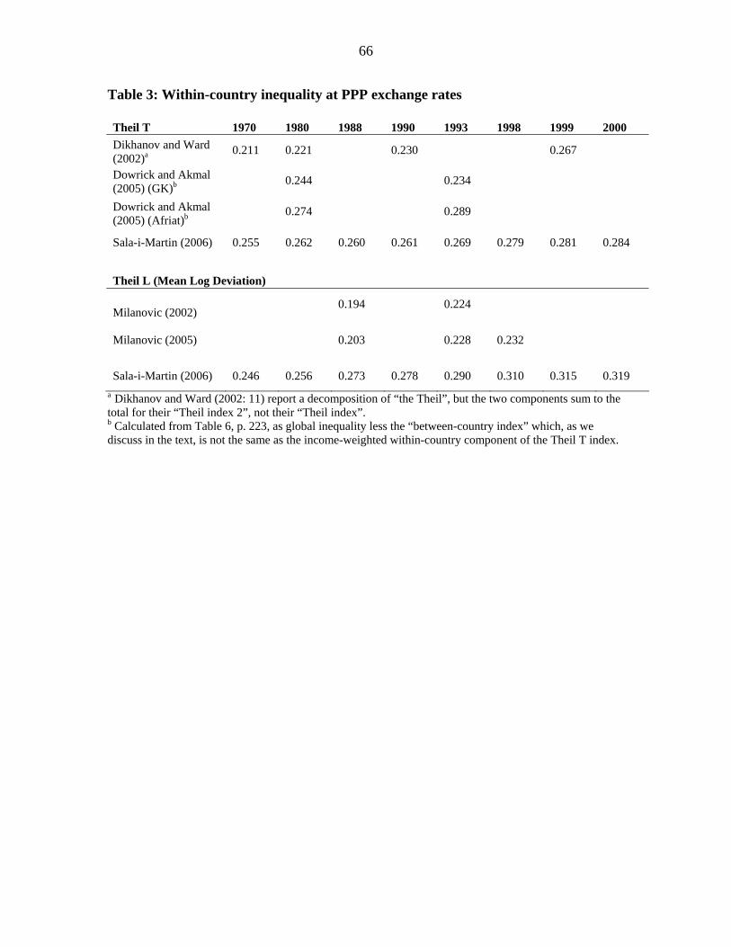
66
Table 3: Within-country inequality at PPP exchange rates Theil T 1970 1980 1988 1990 1993 1998 1999 2000 Dikhanov and Ward (2002)a 0.211 0.221 0.230 0.267
Dowrick and Akmal
(2005) (GK)b 0.244 0.234
Dowrick and Akmal (2005) (Afriat)b 0.274 0.289
Sala-i-Martin (2006) 0.255 0.262 0.260 0.261 0.269 0.279 0.281 0.284
Theil L (Mean Log Deviation)
Milanovic (2002) 0.194 0.224
Milanovic (2005)
0.203 0.228 0.232
Sala-i-Martin (2006) 0.246 0.256 0.273 0.278 0.290 0.310 0.315 0.319 a Dikhanov and Ward (2002: 11) report a decomposition of “the Theil”, but the two components sum to the total for their “Theil index 2”, not their “Theil index”. b Calculated from Table 6, p. 223, as global inequality less the “between-country index” which, as we discuss in the text, is not the same as the income-weighted within-country component of the Theil T index.