gis in ecology
TRANSCRIPT
GIS IN ECOLOGY:
ANALYZING VECTOR DATA
Analyzing Vector Data April 2015
Contents Introduction ...................................................... 2
Vector Tools and Functionality ..................... 2 Course Data Sources ................................... 3
Tasks ............................................................... 4 Getting Started ............................................. 4 Adding XY Data, Joining Data, and Calculating Attributes ................................... 5 Geoprocessing and Summarizing ................ 9 ModelBuilder .............................................. 12
This is an applied course on how to use the software. It reinforces working with map documents and layers. It focuses on overlaying, buffering, and other simple analyses involving vector data, with an introduction to geoprocessing using ArcToolbox and ModelBuilder. For additional suggested reading on GIS theory, fundamentals, and software see: www.esri.com and www.biology.ualberta.ca/facilities/gis/index.php?Page=338#online. Training courses: www.biology.ualberta.ca/facilities/gis/index.php?Page=484#virtualcampus
Learning ArcGIS
Geoprocessing with ArcGIS Desktop
References:
Longley, Paul A., Michael F. Goodchild, David J. Maguire,
and David W. Rhind. 2001. Geographic Information Systems and Science. John Wiley
& Sons, Ltd. Chichester UK. Mitchell, Andy. 1999. The ESRI Guide to GIS Analysis.
Volume 1: Geographic Patterns and Relationships. Environmental Systems
Research Institute, Inc. ESRI. 2015. What is Geoprocessing? Online:
http://desktop.arcgis.com/en/desktop/latest/main/analyze/what-is-geoprocessing.htm
GIS in Ecology is sponsored by the Alberta Cooperative Conservation Research Unit
http://www.biology.ualberta.ca/accru
Analyzing Vector Data April 2015
GIS IN ECOLOGY:
ANALYZING VECTOR DATA
Introduction In this short course you will get familiar with ESRI’s ArcGIS software and its basic functions for spatial analyses on data stored in the vector data model. Recall that vector data represents features as points (x, y coordinates), lines (sets of coordinates), and polygons (sets of coordinates defining boundaries that enclose areas), and focuses on modeling discrete features with precise shapes and boundaries. Example file types include vector coverages, shapefiles, CAD, etc.
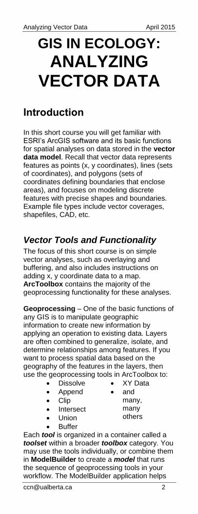
Vector Tools and Functionality The focus of this short course is on simple vector analyses, such as overlaying and buffering, and also includes instructions on adding x, y coordinate data to a map. ArcToolbox contains the majority of the geoprocessing functionality for these analyses. Geoprocessing – One of the basic functions of any GIS is to manipulate geographic information to create new information by applying an operation to existing data. Layers are often combined to generalize, isolate, and determine relationships among features. If you want to process spatial data based on the geography of the features in the layers, then use the geoprocessing tools in ArcToolbox to:
Dissolve
Append
Clip
Intersect
Union
Buffer
XY Data
and many, many others
Each tool is organized in a container called a toolset within a broader toolbox category. You may use the tools individually, or combine them in ModelBuilder to create a model that runs the sequence of geoprocessing tools in your workflow. The ModelBuilder application helps
Toolbox
Toolset
Tool
Script
Model
Analyzing Vector Data April 2015
you to streamline your workflow and automate repetitive tasks by stringing processes together. You may then run the model with a single click, set parameters, iterate, and even export and modify as a script, to adapt your model for flexible applications. Consult the ArcGIS Desktop Help for details on these and many other geoprocessing tools.
Course Data Sources Free spatial data that can be used for GIS analysis in ecological applications have been obtained from the GeoGratis website http://geogratis.cgdi.gc.ca and Alberta SRD www.srd.alberta.ca/Wildfire/WildfireStatus/Historical
WildfireInformation/SpatialWildfireData.aspx. The following summarizes the metadata for each geographic layer in the course dataset that has been made available to you on the local server \COURSES\GIS-100\2_AVD: The 1:250,000 scale data have been previously processed, projected in the NAD 1983 UTM Zone 11 spatial referencing (i.e. map units are in meters) and converted to file geodatabase feature classes for NTS map sheet 083J (Whitecourt) in central Alberta.
Analyzing Vector Data April 2015
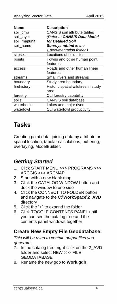
Name Description
soil_cmp soil_layer soil_mapunit soil_name
CANSIS soil attribute tables (Refer to CANSIS Data Model for Detailed Soil Surveys.mhtml in the \_documentation folder.)
sites.xls Locations of field sites
points Towns and other human point features
access Roads and other human linear features
streams Small rivers and streams
boundary Study area boundary
firehistory Historic spatial wildfires in study area
forestry CLI forestry capability
soils CANSIS soil database
waterbodies Lakes and major rivers
waterfowl CLI waterfowl productivity
Tasks Creating point data, joining data by attribute or spatial location, tabular calculations, buffering, overlaying, ModelBuilder.
Getting Started 1. Click START MENU >>> PROGRAMS >>>
ARCGIS >>> ARCMAP 2. Start with a new blank map 3. Click the CATALOG WINDOW button and
dock the window to one side 4. Click the CONNECT TO FOLDER button
and navigate to the C:\WorkSpace\2_AVD directory
5. Click the “+” to expand the folder 6. Click TOGGLE CONTENTS PANEL until
you can see the catalog tree and the contents panel windows together
Create New Empty File Geodatabase:
This will be used to contain output files you generate. 7. In the catalog tree, right-click on the 2_AVD
folder and select NEW >>> FILE GEODATABASE
8. Rename the new gdb to Work.gdb
Analyzing Vector Data April 2015
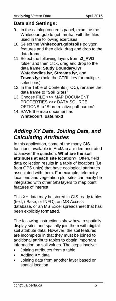
Data and Settings:
9. In the catalog contents panel, examine the Whitecourt.gdb to get familiar with the files used in the following exercises
10. Select the Whitecourt.gdb\soils polygon features and then click, drag and drop to the data frame
11. Select the following layers from \2_AVD folder and then click, drag and drop to the data frame: Study Boundary.lyr, Waterbodies.lyr, Streams.lyr, and Towns.lyr (hold the CTRL key for multiple selections)
12. In the Table of Contents (TOC), rename the data frame to “Soil Sites”
13. Choose FILE >>> MAP DOCUMENT PROPERTIES >>> DATA SOURCE OPTIONS to “Store relative pathnames”
14. SAVE the map document as Whitecourt_date.mxd
Adding XY Data, Joining Data, and Calculating Attributes In this application, some of the many GIS functions available in ArcMap are demonstrated to answer the question: What are the soil attributes at each site location? Often, field data collection results in a table of locations (i.e. from GPS units) that have ecological attributes associated with them. For example, telemetry locations and vegetation plot sites can easily be integrated with other GIS layers to map point features of interest. This XY data may be stored in GIS-ready tables (text, dBase, or INFO), an MS Access database, or an MS Excel spreadsheet that has been explicitly formatted. The following instructions show how to spatially display sites and spatially join them with digital soil attribute data. However, the soil features are incomplete in that they must be joined to additional attribute tables to obtain important information on soil values. The steps involve:
Joining attributes from a table
Adding XY data
Joining data from another layer based on spatial location
Analyzing Vector Data April 2015
TIP: Using Excel for Tables 1. ArcGIS can only read Excel version 2003 or
earlier (no .xlsx files)
2. Only one worksheet can be imported at a time
3. Column headings (field names) must be present
4. Do not use spaces or non-alphanumeric characters in column headings
5. No skipped rows anywhere 6. Be aware that date/time values are subject to
import errors (a work around is to split the date/time parts in to separate columns)
The available data includes tabular point locations and a CANSIS soil survey. (See CANSIS Data Model for Detailed Soil Surveys.mhtml for soil relationship information.) Note: You will notice after completing this task that the soils data are incomplete – i.e. several polygons are unclassified. This demonstrates the point that not all data are equal and that you must check your data for errors/omissions prior to use in analysis!
Join Attributes from Another Table:
The soils coverage has additional attribute tables that must be joined. Use “MAPUNIT” as the field to base the join to attributes from the soil_cmp.dbf table, and then “SOILTYPE” to join attributes from the soil_name.dbf table. 1. Turn off and collapse all but the soils layer 2. Right click on soils and choose JOINS AND
RELATES >>> JOIN 3. In the JOIN DATA wizard at step 1: Choose
“MAPUNIT” 4. At step 2: Click the BROWSE button and
navigate to \2_AVD\Whitecourt.gdb and select the soil_cmp table
5. At step 3: Choose “MAPUNIT” 6. Click OK Repeat a second join on soils using “SOILTYPE” to join attributes with soil_name. Another way to set an attribute join is in Layer Properties. 7. Double click on soils to access its layer
properties 8. In the JOINS & RELATES tab, click on the
ADD button 9. At step 1: Choose “SOILTYPE” 10. At step 2: BROWSE for soil_name 11. At step 3: Choose “SOILTYPE” 12. Click OK twice
Analyzing Vector Data April 2015
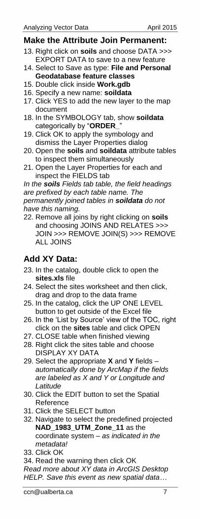
Make the Attribute Join Permanent:
13. Right click on soils and choose DATA >>> EXPORT DATA to save to a new feature
14. Select to Save as type: File and Personal Geodatabase feature classes
15. Double click inside Work.gdb 16. Specify a new name: soildata 17. Click YES to add the new layer to the map
document 18. In the SYMBOLOGY tab, show soildata
categorically by “ORDER_” 19. Click OK to apply the symbology and
dismiss the Layer Properties dialog 20. Open the soils and soildata attribute tables
to inspect them simultaneously 21. Open the Layer Properties for each and
inspect the FIELDS tab In the soils Fields tab table, the field headings are prefixed by each table name. The permanently joined tables in soildata do not have this naming. 22. Remove all joins by right clicking on soils
and choosing JOINS AND RELATES >>> JOIN >>> REMOVE JOIN(S) >>> REMOVE ALL JOINS
Add XY Data:
23. In the catalog, double click to open the sites.xls file
24. Select the sites worksheet and then click, drag and drop to the data frame
25. In the catalog, click the UP ONE LEVEL button to get outside of the Excel file
26. In the ‘List by Source’ view of the TOC, right click on the sites table and click OPEN
27. CLOSE table when finished viewing 28. Right click the sites table and choose
DISPLAY XY DATA 29. Select the appropriate X and Y fields –
automatically done by ArcMap if the fields are labeled as X and Y or Longitude and Latitude
30. Click the EDIT button to set the Spatial Reference
31. Click the SELECT button 32. Navigate to select the predefined projected
NAD_1983_UTM_Zone_11 as the coordinate system – as indicated in the metadata!
33. Click OK 34. Read the warning then click OK Read more about XY data in ArcGIS Desktop HELP. Save this event as new spatial data…
Analyzing Vector Data April 2015
35. In the table of contents, right-click on the sites Event name
36. Select DATA >>> EXPORT DATA 37. Provide a new name for the feature class;
e.g. \Work.gdb\sites 38. Click OK 39. Compare the attribute tables and layer
properties for the sites Events and sites feature class
40. Right click on the name and REMOVE the sites Events and table from the TOC
Join Data from Another Layer Based on Spatial Location:
A spatial join may be used to extract the values from the soildata layer that coincide with the sites locations. 41. Right click on Sites and choose JOINS
AND RELATES >>> JOIN 42. Choose to ‘Join data from another layer
based on spatial location’ and set the following:
43. Step 1: Select soildata as the join layer 44. Step 2: Select ‘it falls inside’ 45. Step 3: Type in an output file name; e.g.
\Work.gdb\soilsites 46. Click SAVE and OK 47. Click YES to add the new point layer to your
map document 48. Open the attribute table to view each
location’s soil attribute values The soilsites layer represents the spatial coincidence of the sites point locations with the soils attributes.
49. SAVE your map document Spatial joins have much power depending on the order (e.g. polygons to points, points to polygons, etc.), and by choice: POLYGONS TO POINTS:
'it falls inside' – this method assigns the attributes of the polygon to the point
'is closest to it' – this method assigns a distance value in a new DISTANCE field
POINTS TO POLYGONS:
'Each polygon will be given a summary of the numeric attributes of the points that fall inside it..." – this method assigns a count value to a new COUNT field
'Each polygon will be given all the attributes of the point that is closest to its boundary..." – this method assigns a distance value in a new DISTANCE field
Analyzing Vector Data April 2015
You can also join points to lines, lines to points, lines to polygons, and polygons to lines! Remember a spatial join is what you use to get counts, intersect points with other layers, or automatically calculate nearest distance measures between features.
Geoprocessing and Summarizing The following instructions show how ArcToolbox’s geoprocessing tools can be used to answer the question: How much waterfowl habitat is within 250 meters of major roads? The steps involve:
Selecting by attributes for major roads
Buffering
Clipping
Calculating area
Summarizing area by habitat class The available data includes a CLI classification on land capability for waterfowl and an access layer including roads. This new analysis will be performed in a new data frame. 1. Choose INSERT >>> DATA FRAME 2. Rename this new data frame: “Waterfowl
Area” 3. Add the following data by dragging and
dropping from the Catalog Name window to the data frame:
Access.lyr
Waterfowl.lyr 4. Click to show the ARCTOOLBOX window
button and dock it where you prefer 5. Take a moment to examine the ArcToolbox
window Keep in mind that there are many ways to utilize ArcToolbox: first you will learn how easy it is to interact with your data in ArcMap using the tools one at a time. Remember to click the Show Help button to view instructions and tips on how to use the tools.
Select By Attributes for Major Roads:
6. Choose DATA MANAGEMENT TOOLS >>> LAYERS AND TABLE VIEWS >>> SELECT LAYER BY ATTRIBUTES
7. Set Access as the layer 8. Click the SQL button 9. Click the appropriate buttons to enter the
expression: "FIR_ROADNO" <> ' '
Recall what you learned in the “Querying in GIS” course.
Analyzing Vector Data April 2015
10. Click OK twice – the primary roads are now highlighted
Buffer:
11. In ArcToolbox, navigate to ANALYSIS TOOLS >>> PROXIMITY >>> BUFFER
12. Double click on the BUFFER tool to open it (alternatively, right click and choose OPEN)
13. Click on the SHOW HELP button – to see helpful information at the right side as you click on each of the parameters on the left side
14. Reposition the Buffer window so you can see it and the TOC simultaneously
15. Click and drag Access from the TOC in ArcMap to the Input Features text box of the Buffer window
16. Specify C:\WorkSpace\2_AVD\Work.gdb\ roadbuffer250 as the Output
17. Enter 250 for the linear distance and select Meters for the unit
18. Select ALL as the Dissolve Type 19. Click OK 20. CLEAR SELECTED FEATURES 21. Zoom in to examine the new roadbuffer250
polygon layer
Clip:
22. In ArcToolbox, navigate to ANALYSIS TOOLS >>> EXTRACT >>> CLIP
23. Double click on the CLIP tool – read the descriptive text that is displayed in the help panel to learn more about this tool
24. Drag Waterfowl to the Input Features layer 25. Drag RoadBuffer250 as the Clip features
layer 26. Specify \2_AVD\Work.gdb\
roadhabitatclip as the output 27. Click OK 28. Zoom in to examine the new
roadhabitatclip layer
Calculate Area:
An attribute table can be treated just like a database table: fields can be added, deleted, and calculated to yield new information about the associated geographic features. In this example, you will update the area field to reflect the actual area of each polygon within the buffers you processed above in preparation for summarizing the data below. 29. SAVE your map document
Analyzing Vector Data April 2015
30. Choose CUSTOMIZE >>> TOOLBARS >>> EDITOR to add it
31. Choose EDITOR >>> START EDITING 32. Select the \Work.gdb to edit data from 33. Right click on roadhabitatclip and OPEN
ATTRIBUTE TABLE 34. Right click on the heading of the “AREA”
field 35. Click CALCULATE GEOMETRY 36. Select the AREA property and Square
Meters (sq m) as the units 37. Click OK 38. Choose EDITOR >>> STOP EDITING 39. Click YES to save edits
IMPORTANT NOTE: Notice that the AREA field now has the exact same values as the SHAPE_AREA field that is automatically generated for geodatabase feature classes. You may want a previous area to persist in future overlay outputs, so calculating your own distinctive field will help with future proportion calculations, for example. However, when working with shapefiles, the automatic geometry fields are not added/calculated, and you must always calculate the geometry into a new or existing field.
Summarize Area by Habitat Class:
40. In the attribute table of roadhabitatclip, right-click on the “CLASS_A” heading
41. Choose SUMMARIZE from the menu 42. Select to summarize CLASS_A by AREA –
Sum (expand and click a check beside Sum)
43. Save to the Work.gdb and specify a name for the output table; e.g. roadhabitatarea
44. Click OK 45. Click YES to add the table to the map
document 46. In the table of contents’ SOURCE tab, open
the roadhabitatarea table to view the info 47. Optionally, right-click the Sum_AREA
heading and click STATISTICS to view Min, Max, Sum (useful for calculating proportions in a new field), Mean, Std Dev
Analyzing Vector Data April 2015
ModelBuilder The following instructions show how ArcToolbox’s ModelBuilder can be used to answer: What is the area of burned riparian forest species for each year? The steps involve:
Setting up a model with ArcToolbox’s ModelBuilder
Buffering water features
Intersecting riparian, forestry and fire history
Adding a field, calculating area, and summarizing multiple fields
Running the model The available data includes streams, water bodies, a CLI classification on land capability for forestry, and fire history layer of polygons indicating the year of burn. This new analysis will be performed in a new data frame 1. Choose INSERT >>> DATA FRAME 2. Rename this new data frame: “Riparian
Fire” 3. From the Catalog, add the following data
from the \2_AVD folder by dragging and dropping to the data frame: Fire History.lyr, Forestry.lyr, and Streams.lyr
4. In the List by Drawing Order view if the TOC, modify the layer drawing order
5. SAVE your map document
Set up ModelBuilder:
To create a model in ModelBuilder, ideally you may create your own custom toolbox in ArcToolbox – there are a few ways to do this, but a good practice is to store it in your working directory for ease of retrieval and sharing. 6. In ArcToolbox, right click on the name
ArcTolbox and choose ADD TOOLBOX 7. Navigate to the \2_AVD folder and click the
NEW TOOLBOX icon 8. Rename Toolbox to “AVD” 9. Highlight it and click OPEN 10. Right click on the AVD toolbox in the
ArcToolbox window and choose NEW >>> MODEL
The ModelBuilder interface is immediately displayed. 11. Choose MODEL >>> MODEL
PROPERTIES 12. In the GENERAL tab, specify a Name (no
spaces) and Labe (spaces okay)l; i.e. RiparianFire
13. Check to ‘Store relative path names’ 14. Click OK
Analyzing Vector Data April 2015
15. Briefly, examine the ModelBuilder window 16. Click OK and then click the SAVE button 17. Choose HELP >>> ARCGIS DESKTOP
HELP 18. Read through ‘What is ModelBuilder’ and
explore some of the links 19. Minimize the help file when finished – you
will want to refer to it as you work
Buffer Water Features:
The first step in your model building is to buffer the water features. 20. In ArcToolbox, navigate to ANALYSIS
TOOLS >>> PROXIMITY >>> BUFFER 21. Drag and drop the BUFFER tool to the
Model window 22. Double click the BUFFER tool element
Specify the input as Streams
Specify the output as \Work.gdb\streams_Buffer
Set the Distance linear unit to 500 meters
Dissolve ALL and leave all else at their defaults
Click OK 23. Click on the AUTO LAYOUT and
FULL EXTENT buttons to organize the model elements
You could run the model at this point, but to see just how powerful and timesaving ModelBuilder is, continue with building your model until all processes have been set up.
Intersect Riparian, Forestry and Fire History:
24. In ArcToolbox, navigate to ANALYSIS TOOLS >>> OVERLAY >>> INTERSECT
25. Drag and drop the INTERSECT tool to the Model window
26. Double click on the INTERSECT tool element to open it
Specify Fire History, Forestry and streams_Buffer as the input features
Change the output name to \Work.gdb\ riparianfirespecies
Click OK
Add, Calculate, and Summarize Fields:
27. Use the SEARCH and/or INDEX tabs in ArcToolbox to locate the tool you want
Analyzing Vector Data April 2015
28. Locate, drag, and drop the ADD FIELD tool to the Model window
29. Connect the INTERSECT output to the ADD FIELD tool
30. Double click on the ADD FIELD tool element to open it
Specify the new Field Name as I_AREA
Specify the Field Type as DOUBLE
Click OK 31. Repeat the locate, drag, and drop for the
CALCULATE FIELD tool 32. Double click CALCULATE FIELD to open it
Specify the input table as riparianfirespecies (2)
Specify the new Field Name as I_AREA
Specify the Expression as !shape.area!
Select the Expression Type as PYTHON_9.3
Click OK 33. Repeat the locate, drag, and drop for the
SUMMARY STATISTICS tool 34. Double click SUMMARY STATISTICS to
open it
Specify the input
Specify the output table as \Work.gdb\ yearspeciesarea
Select I_AREA – SUM for the Statistics Field(s)
Select BURNYEAR and SPECIES_A1 for the Case Field(s)
Click OK
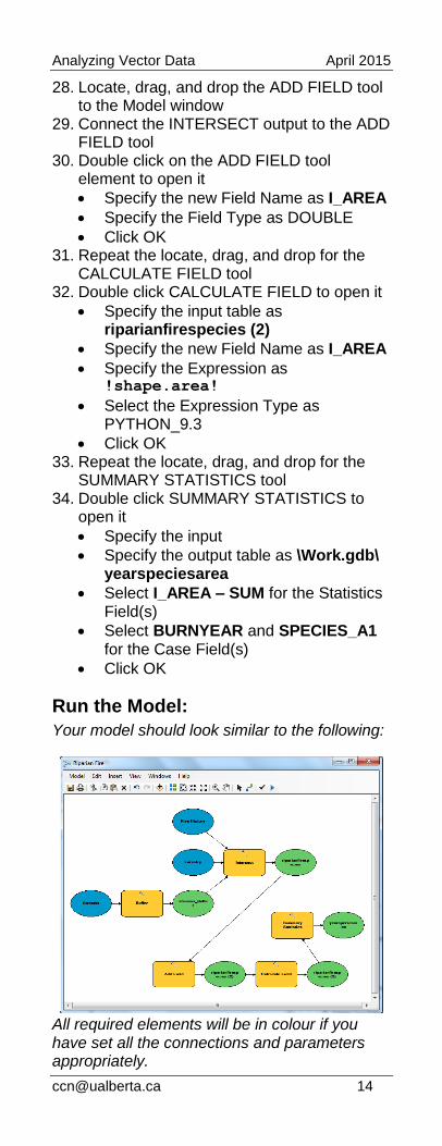
Run the Model:
Your model should look similar to the following:
All required elements will be in colour if you have set all the connections and parameters appropriately.
Analyzing Vector Data April 2015
If not, simply double click on each element to open, examine, and modify as necessary. 35. Click on the SAVE button (perhaps this is a
good time to SAVE the map document, too) 36. Choose MODEL >>> VALIDATE ENTIRE
MODEL – all model elements should be in color
37. Choose MODEL >>> RUN ENTIRE MODEL – or click on the RUN button
38. After waiting for the processes to complete, examine the log window then close
39. In the ModelBuilder window, right click on the final output yearspeciesarea and choose ADD TO DISPLAY
You may examine the intermediate layers by adding them to ArcMap or preview them in ArcCatalog. If you are satisfied with the final output then you may opt to delete all intermediate data. 40. Make any modifications to the model; e.g.
UNcheck ‘Intermediate’ for the riparian and riparianfirespecies outputs (right click on each to access this)
41. Choose MODEL >>> DELETE INTERMEDIATE DATA
42. Click SAVE and close the ModelBuilder window
43. Copy the entire 2_AVD folder to a backup location or zip and email to yourself
Note: For future reference, know that you can set the ARCTOOLBOX >>> ENVIRONMENT working directory and other options. You now have the knowledge and experience to apply any geoprocessing tool to vector data, one at a time, or efficiently strung together in a process that is reproducible and documented.