gis-e1070 theories and techniques in gis d

GIS-E1070 Theories and Techniques in GIS D

Lecture 5: Map Algebra and raster data indexing

Jussi Nikander

The contents of this lecture

• Map Algebra

• Functions in map algebra as defined by Tomlin

• Map algebra definition vs. implementations

Learning goals of this lecture

Be able to use the different map algebra functions

Understand the similarities and differences between map algebra

definition and implementation

Be able to search for map algebra functionality in GIS software

Literature for this lecture

• C. Dana Tomlin: Geographic Information Systems and

Cartographic Modeling

• Yes, the whole book is about map algebra. No, you don’t need to read it for the exam.

Raster data analysis using map algebra

Introduction to raster data

• Raster data model

• Geographic data modelled by dividing it into a regular tessellation that is made of pixels

• Each pixel has a location and a value

• Often, real data is collected from discrete points

• In such case individual pixel values are then interpolated from the data

• Increasingly data can be gathered with sufficient resolution to not require interpolation for many applications

• Raster data is similar to normal images• Therefore image processing

methods could, in theory, be used

• Remember, GeoTIFF is just a TIFF image with extra metadata

• Map algebra• Designed for manipulating

spatial data in raster format

Raster data fundamentals

• Raster geometry

• Pixels can be square,

hexagonal, voxels

• Squares most common, voxels in 3D

• Square pixel

• 4 neighbors – joint edge

• 8 neighbors – joint edge or corner

• Hexagonal pixel• 6 neighbors

• Simple pixel neighborhoods in square and hexagon rasters• In the square raster 𝑁𝐴

represents 4-neighborhood and 𝑁𝐵 8-neighborhood

𝑵𝑨

𝑵𝑨 A 𝑵𝑨

𝑵𝑨

𝑵𝑩 𝑵𝑩 𝑵𝑩

𝑵𝑩 B 𝑵𝑩

𝑵𝑩 𝑵𝑩 𝑵𝑩

A

𝑁𝐴

𝑁𝐴

𝑁𝐴

𝑁𝐴𝑁𝐴

𝑁𝐴

Raster data fundamentals

• Raster data has implicit topology• Joint edges imply adjacency• Joint edges or corners

connectivity

• Raster data (with square pixels) can be modelled using a two-dimensional matrix (array)

• Resolution, matrix orientation and origin determine the coordinates of a pixel

• On the left matrix A stands for Adjacent cell and C for

connected cell

• On the right matrix the geogprahic coordinates for

origin are known

• Coordinates for other cell are calculated from that

using cell position (i,j) and the x- and y-offsets (d and

e in the figure): 𝑥𝑖 = 𝑥0 + 𝑑𝑖, 𝑦𝑗 = 𝑦0 − 𝑒𝑗

1,0 2,0 3,0 4,0

0,1 1,1 2,1 3,1 4,1

0,2 1,2 2,2 3,2 4,2

0,3 1,3 2,3 3,3 4,3

0,4 1,4 2,4 3,4 4,4

C A C

A A

C A C

dOrigin (GeoTIFF)

e

Raster data management

• One raster layer contains one theme• e.g. Soil layer, vegetation layer, height layer

• Pixel values according to the theme

• Layers can be stored as separate files• E.g. geotiff-images with associated

metadata

• ...or in database

• Data can also be compressed• RLE – run-length encoding

• Quad-tree

• (other) image compression methods

• Compare the pixel values in the two rasters above. Does the data tell anything about the phenomena depicted in the rasters?

1 1 22 22 4

1 1 15 15 4

2 1 15 15 9

15 15 9 9 9

15 15 5 9 9

3.4 3.3 3.4 3.5 3.6

3.3 3.3 3.4 3.5 3.6

3.2 3.3 3.3 3.5 3.5

3.0 3.1 3.2 3.4 3.5

2.8 2.9 3.1 3.2 3.3


• One raster layer contains one theme• e.g. Soil layer, vegetation layer, height layer

• Pixel values according to the theme

• Layers can be stored as separate files• E.g. geotiff-images with associated

metadata

• ...or in database

• Data can also be compressed• RLE – run-length encoding

• Quad-tree

• (other) image compression methods

• Left raster might contain categorical (nominal) data?

• And the right measurements (interval or ratio data)?

1 1 22 22 4

1 1 15 15 4

2 1 15 15 9

15 15 9 9 9

15 15 5 9 9

3.4 3.3 3.4 3.5 3.6

3.3 3.3 3.4 3.5 3.6

3.2 3.3 3.3 3.5 3.5

3.0 3.1 3.2 3.4 3.5

2.8 2.9 3.1 3.2 3.3


• Raster queries are generally in the form

• “Select pixels that fulfil condition C (and perform operation O on these pixels)”

• Pixels can be identified by

• Geographic coordinates

• Image coordinates

• Attribute values

• Possible operations are numerous

• Map Algebra is a reasonably complete set of basic operations

• “Select pixels where value=9 on the left raster”

• “Select all pixels in coordinate range (0,0) to (1,4) and add 1 to their value on the right raster”

1 1 22 22 4

1 1 15 15 4

2 1 15 15 9

15 15 9 9 9

15 15 5 9 9

3.4 3.3 3.4 3.5 3.6

3.3 3.3 3.4 3.5 3.6

3.2 3.3 3.3 3.5 3.5

3.0 3.1 3.2 3.4 3.5

2.8 2.9 3.1 3.2 3.3


• Raster queries are generally in the form

• “Select pixels that fulfil condition C (and perform operation O on these pixels)”

• Pixels can be identified by

• Geographic coordinates

• Image coordinates

• Attribute values

• Possible operations are numerous

• Map Algebra is a reasonably complete set of basic operations

• “Select pixels where value=9 on the left raster”

• “Select all pixels in coordinate range (0,0) to (1,4) and add 1 to their value on the right raster”

1 1 22 22 4

1 1 15 15 4

2 1 15 15 9

15 15 9 9 9

15 15 5 9 9

4.4 4.3 3.4 3.5 3.6

4.3 4.3 3.4 3.5 3.6

4.2 4.3 3.3 3.5 3.5

4.0 4.1 3.2 3.4 3.5

3.8 3.9 3.1 3.2 3.3

Raster query examples

• selection according to the attribute• ”give the locations of all pixels with value w”

• selection according to the location• ”give the value of the pixel in location (p,q)

• selection according to several attributes• ”give the locations of the pixels having the

values a1 > w, a2 > y and a3 = z”

• In this example, there would be three raster layers

• Queries according to topology

• ”Give the attribute values for the neighbours of the pixel in (p,q)”

2 1 5 3 8

0 4 0 3 2

1 0 7 6 5

4 2 3 5 0

6 5 4 2 0

2 1 6 4 0

6 4 3 7 5

9 7 6 5 3

2 7 8 9 0

4 3 5 7 8

T T F T T

F T F F F

F F F F T

T F F F F

T T F F F

𝑣𝑎𝑙𝑢𝑒 > 0 𝑣𝑎𝑙𝑢𝑒 < 5

and

Usually T=1 and F=0

Map algebra

• Created as an algebra for spatial data (stored in raster format)

• Data stored in layers

• Each layer can contain different type of data

• Map algebra operation takes as input a number of existing layers

• Mathematical (arithmetic and/or logical) operations done based on the layer data

• As output it produces a new map layer

• More details on the use of map algebra covered on the course GIS-E1060

• In map algebra there are four different types

of functions

• Local functions

• Focal functions

• Zonal functions

• Incremental functions

• Originally proposed by Dr. Dana Tomlin in the

1980s

• NOT a standard defined by any international

standardization organization!

• Thus, there isn’t a consensus on what a map

algebra implementation should include

Map algebra function types

• Local functions• New value based on values of a single

pixel on one or more input layers

• Focal functions• New value based on values of a pixel’s

neighbourhood on input layer (e.g. 3x3, 5x5)

• Neighbourhood can be defined using 4-neighbours or 8-neighbours

• Or cumulative sum of distances, 3d surface, or according to a graph, etc.

• Zonal functions

• New value based on the sum the values on first input layer’s pixels in the zones defined by the second input layer

• Incremental functions

• New value based on incrementing the pixel’s lineal, areal etc. value according to the slope, area or lineal condition defined on the input layer

• For example, drainage

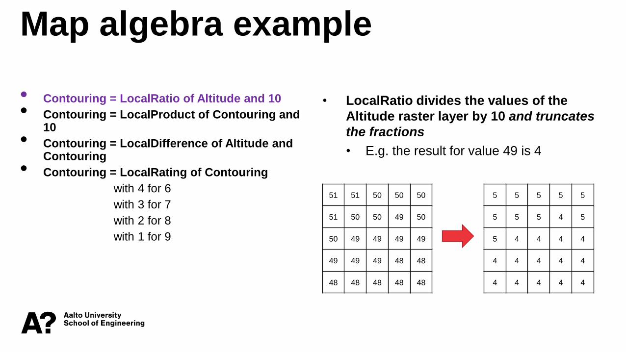
Map algebra example

• Contouring = LocalRatio of Altitude and 10

• Contouring = LocalProduct of Contouring and 10

• Contouring = LocalDifference of Altitude and Contouring

• Contouring = LocalRating of Contouring

with 4 for 6

with 3 for 7

with 2 for 8

with 1 for 9

51 51 50 50 50

51 50 50 49 50

50 49 49 49 49

49 49 49 48 48

48 48 48 48 48

Map algebra example





with 4 for 6

with 3 for 7

with 2 for 8

with 1 for 9

• LocalRatio divides the values of the

Altitude raster layer by 10 and truncates

the fractions

• E.g. the result for value 49 is 4

51 51 50 50 50

51 50 50 49 50

50 49 49 49 49

49 49 49 48 48

48 48 48 48 48

5 5 5 5 5

5 5 5 4 5

5 4 4 4 4

4 4 4 4 4

4 4 4 4 4

Map algebra example





with 4 for 6

with 3 for 7

with 2 for 8

with 1 for 9

• LocalProduct multiplies the result of

the first line by 10

• E.g. 49 turns into 4 and then into 40

5 5 5 5 5

5 5 5 4 5

5 4 4 4 4

4 4 4 4 4

4 4 4 4 4

50 50 50 50 50

50 50 50 40 50

50 40 40 40 40

40 40 40 40 40

40 40 40 40 40

Map algebra example





with 4 for 6

with 3 for 7

with 2 for 8

with 1 for 9

• LocalDifference subtracts the result of

the second line from Altitude, leaving

only the last digit

• E.g. 49 – 40 = 9

50 50 50 50 50

50 50 50 40 50

50 40 40 40 40

40 40 40 40 40

40 40 40 40 40

51 51 50 50 50

51 50 50 49 50

50 49 49 49 49

49 49 49 48 48

48 48 48 48 48

1 1 0 0 0

1 0 0 9 0

0 9 9 9 9

9 9 9 8 8

8 8 8 8 8

- =

Map algebra example





with 4 for 6

with 3 for 7

with 2 for 8

with 1 for 9

• LocalRating reclassifies the

values: 4 is substituted for 6, 3

for 7, 2 for 8 and 1 for 9

1 1 0 0 0

1 0 0 9 0

0 9 9 9 9

9 9 9 8 8

8 8 8 8 8

1 1 0 0 0

1 0 0 1 0

0 1 1 1 1

1 1 1 2 2

2 2 2 2 2

Map algebra example





with 4 for 6

with 3 for 7

with 2 for 8

with 1 for 9

• The result is a map layer with values

0-5 representing one meter altitude

contours that can be visualized

using e.g. different shades of gray

1 1 0 0 0

1 0 0 1 0

0 1 1 1 1

1 1 1 2 2

2 2 2 2 2

Map algebra example: in summary





with 4 for 6

with 3 for 7

with 2 for 8

with 1 for 9

• LocalRatio divides the values of the Altitude raster

layer by 10 and truncates the fractions

• E.g. the result for value 49 is 4

• LocalProduct multiplies the result of the first line by 10

• E.g. 49 turns into 4 and then into 40

• LocalDifference subtracts the result of the second line

from Altitude, leaving only the last digit

• E.g. 49 – 40 = 9

• LocalRating reclassifies the values: 4 is substituted

for 6, 3 for 7, 2 for 8 and 1 for 9

• The result is a map layer with values 0-5 representing

one meter altitude contours that can be visualized

using e.g. different shades of gray

Local operations

• Local…

• Trigonometric functions (sin, cos, tan, arcsin, arccos, arctan)

• Arithmetic functions (sum, difference, product, ratio, root)

• Statistical functions (maximum, minimum, majority, minority, mean, variety)

• Set functions (combination)

• Reassignment functions (rating)

• NEWLAYER is the function output

• FUNCTION is one of the defined

functions

• E.g. localsum, localminority

• FIRSTLAYER (and NEXTLAYERs, if

applicable) are the input layers

• The function is applied to the value

of every location (pixel) separately

NEWLAYER = localFUNCTION of FIRSTLAYER [and NEXTLAYER]*

Local operations

• Trigonometric functions

• Take one input layer, do the trigonometric operation separately for each value

• Arithmetic functions

• Take at least two layers as input, do the arithmetic on them

• Difference subtracts the value of each NEXTLAYER from the FIRSTLAYER• LocalDifference of 𝐴 and 𝐵 and 𝐶 = 𝐴 − 𝐵 − 𝐶

• Ratio divides FIRSTLAYER by each NEXTLAYER in turn• LocalRatio of 𝐴 and 𝐵 and 𝐶 = Τ𝐴 Τ𝐵 𝐶

• Τ0 0 = 0, Τ𝐴 0 = ∞, Τ−𝐴 0 = −∞ (𝐴 > 0)

• Root takes the root on FIRSTLAYER, where the root to use is specified by (the product of) NEXTLAYER(s)• LocalRoot of 𝐴 and 𝐵 =

𝐵𝐴

• LocalRoot of 𝐴 and 𝐵 and 𝐶 =𝐵𝐶

𝐴

• Statistical operations

• Take at least two layers as input, do the appropriate statistics

for each pixel location separately

• Maximum specifies that the value at a location is the largest of

the input layers’ values at the location (similarly minimum)

• Mean specifies the average

• Variety specifies the number of distinct input values

• Majority specifies the input value with most occurrences. Or

error, if more than one such value is found

• Minority specifies the input value with least occurrences (or

error)

• Combination specifies a particular combination of values from

input layers

• The raster values in the output are assigned according to

order of the combinations sorted by minimum value

• Rating reassigns output layer values according to parameters

Local operation classroom exercise

layerC = localProduct of layerA and layerB

layerA layerB layerC

1 1 1 0.9 0.9

1 0.9 0.9 0.7 0.7

0.9 0.6 0.7 0.7 0.7

0.7 0.6 0.6 0.7 0.7

0.7 0.6 0.6 0.5 0.5

0 0.2 0.3 0.5 0.5

0.4 0.4 0.5 0.5 0.4

0.4 0.4 0.4 0.3 0.3

0.3 0.3 0.2 0.2 0.3

0.4 0.3 0.3 0.3 0.3

Local operation classroom exercise

1 1 1 0.9 0.9

1 0.9 0.9 0.7 0.7

0.9 0.6 0.7 0.7 0.7

0.7 0.6 0.6 0.7 0.7

0.7 0.6 0.6 0.5 0.5

0 0.2 0.3 0.5 0.5

0.4 0.4 0.5 0.5 0.4

0.4 0.4 0.4 0.3 0.3

0.3 0.3 0.2 0.2 0.3

0.4 0.3 0.3 0.3 0.3

0 0.2 0.3 0.45 0.45

0.4 0.36 0.45 0.35 0.28

0.36 0.24 0.28 0.21 0.21

0.21 0.18 0.12 0.14 0.21

0.28 0.18 0.18 0.15 0.15

layerC = localProduct of layerA and layerB


Implementation of local operations

• As specified by Tomlin, map algebra includes only algebraic operations

• So there’s no LocalLessThanor LocalLargerThan

• Or LocalAnd or LocalOr

• In practice, the specification is followed loosely, such as in ArcGIS Desktop raster calculator

Implementation of local operations

• As specified by Tomlin, map algebra includes only algebraic operations

• So there’s no LocalLessThanor LocalLargerThan

• Or LocalAnd or LocalOr

• In practice, the specification is followed loosely, such as in ArcGIS Desktop raster calculator

Raster input layers

Constant “rasters”

Basic

Arithmetic

Comparison

Basic logic

(and, or,

xor, not)

Parentheses

Conditional,

math, trigonometric,

etc. operations

Actual map algebra

expression goes here

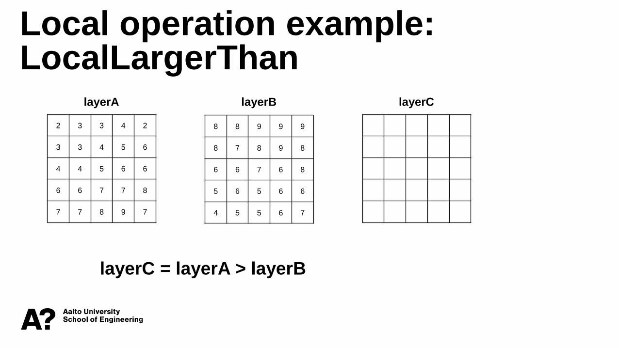
Local operation example: LocalLargerThan

2 3 3 4 2

3 3 4 5 6

4 4 5 6 6

6 6 7 7 8

7 7 8 9 7

8 8 9 9 9

8 7 8 9 8

6 6 7 6 8

5 6 5 6 6

4 5 5 6 7

layerC = layerA > layerB


Local operation example: LocalLargerThan

2 3 3 4 2

3 3 4 5 6

4 4 5 6 6

6 6 7 7 8

7 7 8 9 7

8 8 9 9 9

8 7 8 9 8

6 6 7 6 8

5 6 5 6 6

4 5 5 6 7

F F F F F

F F F F F

F F F F F

T F T T T

T T T T F

layerC = layerA > layerB


Focal operations

• Focal…

• Statistics functions (majority, maximum, mean, minimum, minority, percentage, percentile, ranking, variety)

• Arithmetic functions (product, sum)• Set functions (combination)• Neighborhood functions (bearing,

gravitation, neighbor, proximity)• Reassignment functions (rating)


• FUNCTION is one of the defined functions

• E.g. focalmajority, focalsum

• FIRSTLAYER is the input layer for the

function

• The rest defines how the pixel neighborhood

is defined

• Distance and direction define the size and

direction(s) of the neighborhood

• Spreading and radiating can be used to

define more complex neighborhoods

• Focal functions are always applied to a

specific pixel and its neighborhood

• The function result in NEWLAYER is stored

in each pixel location

NEWLAYER = FocalFUNCTION of FIRSTLAYER

[at DISTANCE] [by DIRECTION] [spreading…] [radiating…]

Focal operation example: focal sum• This example shows how the

Focalsum function is calculated

• Here the process is shown for one pixel

Focalsum (3x3 neighborhood)

2 1 5 3 8

0 4 0 3 2

1 0 7 6 5

4 2 3 5 0

6 5 4 2 0

2 + 1 + 5 + 0 + 4 + 0 + 1 + 0 + 7 = 20

20

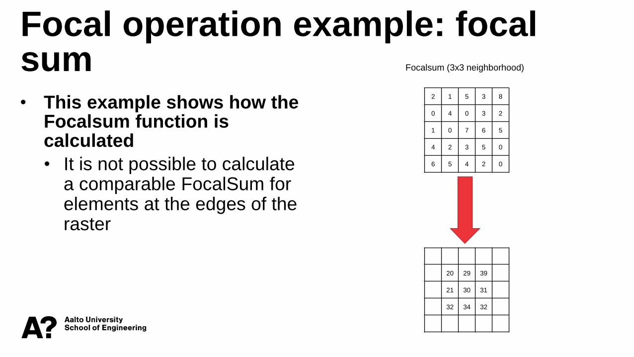
Focal operation example: focal sum• This example shows how the

Focalsum function is calculated

• It is not possible to calculate a comparable FocalSum for elements at the edges of the raster

Focalsum (3x3 neighborhood)

2 1 5 3 8

0 4 0 3 2

1 0 7 6 5

4 2 3 5 0

6 5 4 2 0

20 29 39

21 30 31

32 34 32

Focal operations

• Focal operations are always applied to one layer within

a specified neighborhood window

• E.g. rectangular 3x3 neighborhood

• Result is always stored in the center pixel

• Focal arithmetic

• Adds or multiplies all values within the window

• FocalSum actually is equivalent to (unnormalized) box

blur filter and can be implemented using convolution

• Combination

• Creates a set of values from the neighborhood for each

pixel in the FIRSTLAYER

• Rating reassigns output layer pixel value according to

FIRSTLAYER neighborhood and other parameters

• Focal statistics

• Measures the appropriate statistics within the neighborhood

• Maximum, minimum, majority, minority, mean, and variety are similar to

corresponding local functions

• The function is merely applied to the neighborhood instead of different input layers

• Percentage measures the number of values in the neighborhood that are

identical to the value of the current pixel (point for which the function is

calculated)

• Percentile measures the number of pixel that are lower than the value of

the current pixel

• Ranking tells the number of distinct values in the neighborhood that are

lower than the value of the current pixel

• Neighbor, route, and cost functions

• Proximity tells the distance to the nearest neighbor with non-null value

• Neighbor tells the value of the nearest neighbor pixel

• Bearing tells the direction of the nearest neighbor

• Gravitation is the average cost distance to neighboring pixels

Implementation of focal operations

• By far the most common implementation of focal operations is on a rectangular window of specific size• 3x3, 5x5, 3x5, etc.

• Focal functions are not the same as convolution filters• With the exception of focalsum

which corresponds to box blur convolution (all onesconvolution matrix)

• How and where focal operations are

implemented depends on the software

• E.g. ArcGIS Desktop has a focal

statistics tool that includes (many) of the

focal functions defined for map algebra

Zonal operations

• Zonal...

• Statistical functions (Combination, majority, maximum, mean, minimum, minority, percentage, percentile, ranking, variety)

• Arithmetic functions (product, sum

• Rating


• FIRSTLAYER is the input layer for which the function is calculated

• SECONDLAYER defines the zones for which the calculation is done separately

• Zones do not refer to continuous areas, but pixels that have the same value!

NEWLAYER = zonalFUNCTION of FIRSTLAYER [within SECONDLAYER]

Zonal operations

• Zonal statistics

• Calculates the corresponding statistics to all pixels in the each zone

• For zonal percentage the output is the percentage of pixels within the zone that are identical to the current pixel

• For percentile the output is the percentage of pixels that have lower values to the current pixel

• For other functions (majority, minority, etc.), the output layer has the same value in every pixel in the zone

• Compare this to focal functions where each pixel’s neighborhood is considered separately

• Zonal arithmetic

• Sums or multiplies all pixels in each zone together

• Rating again reassigns pixel values

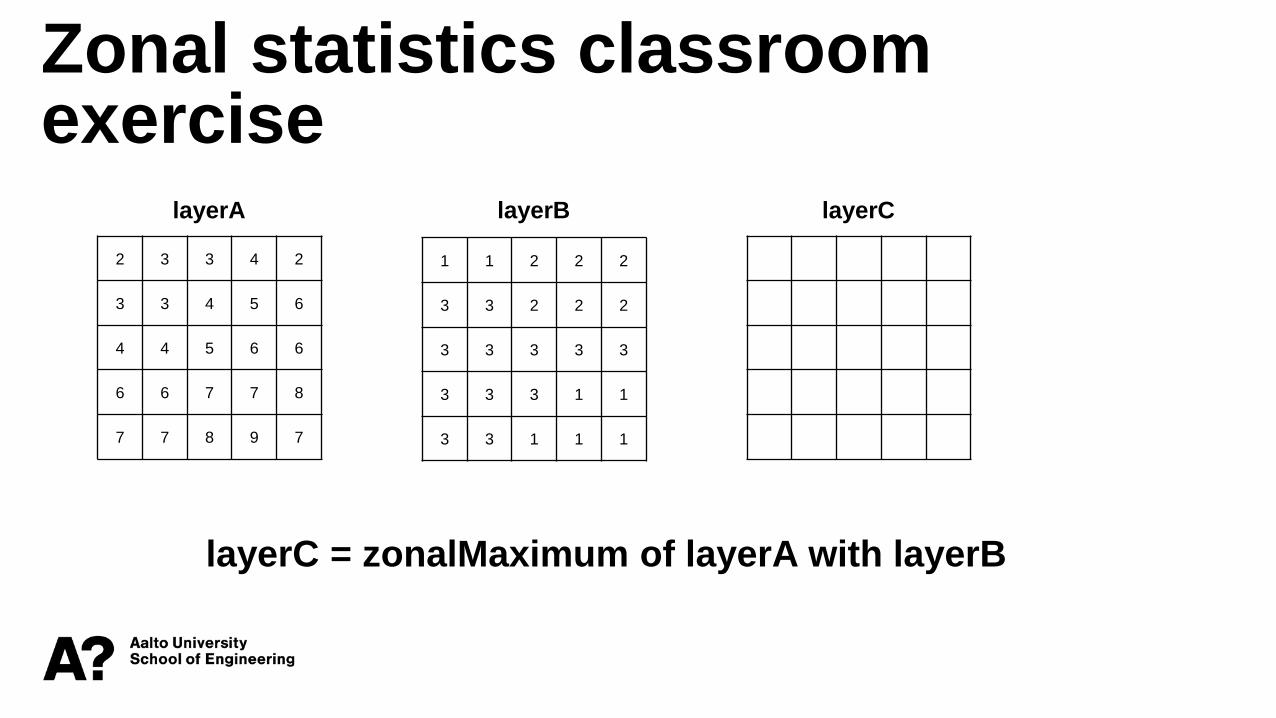
Zonal statistics classroom exercise

2 3 3 4 2

3 3 4 5 6

4 4 5 6 6

6 6 7 7 8

7 7 8 9 7

1 1 2 2 2

3 3 2 2 2

3 3 3 3 3

3 3 3 1 1

3 3 1 1 1

layerC = zonalMaximum of layerA with layerB


Zonal statistics classroom exercise

2 3 3 4 2

3 3 4 5 6

4 4 5 6 6

6 6 7 7 8

7 7 8 9 7

1 1 2 2 2

3 3 2 2 2

3 3 3 3 3

3 3 3 1 1

3 3 1 1 1

9 9 6 6 6

7 7 6 6 6

7 7 7 7 7

7 7 7 9 9

7 7 9 9 9

layerC = zonalMaximum of layerA with layerB


Implementation of zonal operations• The input for zonal

operations requires the zone layer (SECONDLAYER) and input layer (FIRSTLAYER) for which the operation is done

• The operation is then evaluated in each zone separately

• Zones can be non-continuous

• ArGIS Desktop includes a zonal statistics tool

Incremental operations

• Incremental…

• Linear operations (linkage, length)

• Areal operations (area, aspect, drainage, frontage, gradient, partition, volume)

• Newlayer is the output

• Firstlayer is the thematic input layer

• E.g. a road network

• Not used by all functions

• Surfacelayer is the elevation input layer

• Not used by all functions

NEWLAYER = incrementalFUNCTION [of FIRSTLAYER] [on SURFACELAYER]


• Linear operations• Work on input layers that

represent networks• Calculate explicit linkage and

edge length

• Slope-related functions• Aspect is the compass direction of

the steepest slope• Gradient is the degree of the slope• Drainage tells from which adjacent

neighbors water flows into the pixel

• Area and volume• These functions calculate the

area/volume defined by a pixel and its neighbors

• Volume is calculated against a defined plane (e.g. sea-level)

• Frontage and partition• Calculate the length (frontage)

and type (partition) of the boundary the pixel has with other areas


• Incremental operations are more linked to spatial analysis tasks instead of being general mathematical functions with 2-dimensional operands

• A common theme is to make local calculations that, when repeated over the whole input layer(s), create a global effect

• For exampleIncrementalLinkage –function • takes as input a map layer

representing a network of linear elements

• Creates as output a map layer representing explicit network of these elements

• For example, from a layer representing road/not road, it creates a layer representing the road network

IncrementalLinkage and IncrementalLength

• IncrementalLength takes the result of

IncrementalLinkage and a layer

representing surface elevation, and

calculates the length of each

segment created by Linkage

• The end result of these two functions

is thus a raster representation of a

weighted graph (network), where

edge weight is edge length

Image source: Tomlin: Geographic Information Systems

and Cartographic modeling

IncrementalLinkage example

1 1

1 1 1

1

1

1 1 1 1

1 3

36 10 20

9

35

6 19 10 5

layerA

layerB = incrementalLinkage of layerA

layerB

Slope (gradient) and aspect

• Depicted here is one way you can

calculate the local slope and

aspect characteristics• Here, both are calculated using

the 4-neighborhood (𝑧2, 𝑧4, 𝑧6,𝑧8)• And actually without using the current pixel

value at all…

• Remember that result of 𝐺2 +𝐻2 is the tangent of the

slope degree• G is the gradient of the slope in east-west

direction, while H is gradient of the slope in the north-south direction

Image source: Burrough & McDonnell: Principles of Geographical Information Systems

Implementation of incremental operations• As these elements of the map

algebra are related to specific

spatial analysis (network, area,

drainage, boundary) their

implementation is typically spread

in the programs

• I am not aware of any implementation of map algebra that explicitly includes these elements as parts of the algebra as opposed to analysis tools

• ArcGIS Desktop spatial analyst

includes, at least, aspect, slope,

and flow direction• Local flow corresponds to

incrementalDrainage

Summary of map algebra

• The ability to make calculation on rasters

is important part of many spatial analysis

processes

• The original map algebra by Tomlin is not

a something implementations follow

strictly

• Thus for each tool you really need to

check what’s available

• Also, it is important to find out where

each function is in your tool

• Or use the programming environment

Local functions

Zonal statistics

Slope and aspect

Drainage

Focal statistics

Not very conveniently placed if you’d start looking for map

algebra in one place. Also, not all map algebra is in the Map

Algebra toolbox. This is why ArcGIS has search functionality

Questions?

gis-e1070 theories and techniques in gis d

Documents