Runoff  and  geomorphic  properties    of  North  Carolina  rivers  

 Michael  Kanarek  

 Dec.  7,  2012  

 CE  394K.3  

   

Introduction  

Hypsometric  analysis  is  used  in  a  several  geologic  fields,  including  hydrology.  A  

number  of  studies  on  the  relationship  between  hypsometry  and  hydrology  have  

found  that  hypsometric  curve  parameters  have  a  strong  relationship  with  basin  

hydrology,  especially  flood  response.  (Perez-­‐Pena  et  al.,  2009)  GIS  provides  

powerful  tools  for  the  study  of  these  properties,  especially  through  the  utilization  of  

digital  elevation  models.  

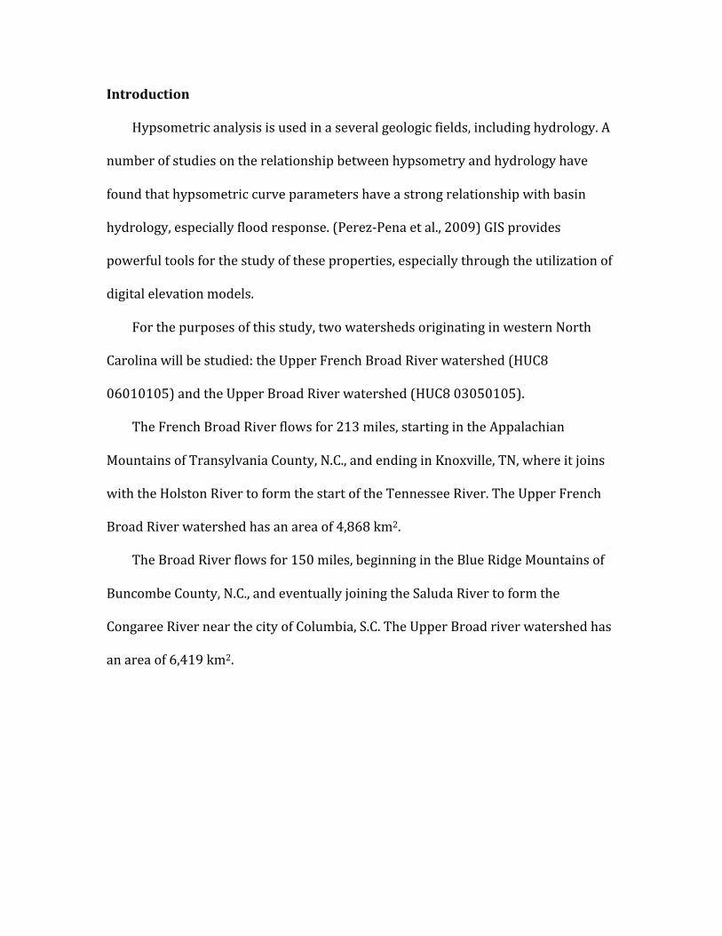
For  the  purposes  of  this  study,  two  watersheds  originating  in  western  North  

Carolina  will  be  studied:  the  Upper  French  Broad  River  watershed  (HUC8  

06010105)  and  the  Upper  Broad  River  watershed  (HUC8  03050105).  

The  French  Broad  River  flows  for  213  miles,  starting  in  the  Appalachian  

Mountains  of  Transylvania  County,  N.C.,  and  ending  in  Knoxville,  TN,  where  it  joins  

with  the  Holston  River  to  form  the  start  of  the  Tennessee  River.  The  Upper  French  

Broad  River  watershed  has  an  area  of  4,868  km2.  

The  Broad  River  flows  for  150  miles,  beginning  in  the  Blue  Ridge  Mountains  of  

Buncombe  County,  N.C.,  and  eventually  joining  the  Saluda  River  to  form  the  

Congaree  River  near  the  city  of  Columbia,  S.C.  The  Upper  Broad  river  watershed  has  

an  area  of  6,419  km2.  

   

   

National Geographic, Esri, DeLorme, NAVTEQ, UNEP-WCMC, USGS, NASA,

ESA, METI, NRCAN, GEBCO, NOAA, iPC

0 10 20 30 405

Miles

WatershedsUpper Broad

Upper French Broad ±

Watershed locations

Data  gathering  

Data  for  this  project  was  acquired  primarily  from  the  USGS’s  National  Map  

Viewer.  Elevation  data  was  downloaded  in  the  form  of  nine  individual    

1/3  arcsecond  digital  elevation  maps.    

Hydrography  data  from  the  National  Hydrography  Dataset  were  also  found  

through  the  National  Map  Viewer.  This  data  contained  watershed  boundaries  that  

allowed  for  delineation  of  these  watersheds  as  well  as  flowline  data  for  all  streams  

within.    

Precipitation  and  stream  discharge  data  were  gathered  from  the  National  Water  

Information  System  (NWIS).  

   

Data  processing  

In  order  to  work  with  a  cohesive  DEM,  the  nine  individual  tiles,  in  GeoTIFF  

format,  were  stitched  together  using  the  Mosaic  to  New  Raster  tool  in  ArcGIS.  This  

allows  for  a  uniform  shading  scale  to  be  used  across  the  study  areas.  

Given  the  high  resolution  of  this  DEM,  before  any  further  processing  of  the  DEM  

took  place,  it  was  clipped  to  just  the  two  watersheds  being  considered  to  save  on  

processing  time.  The  Extract  by  Mask  tool  and  the  previously  delineated  watershed  

boundaries  were  used  in  this  task.  Then,  the  Fill  tool  was  used  to  eliminate  pits  from  

the  DEM,  and  its  symbology  was  altered  to  use  a  color  gradient  to  represent  the  

changes  in  elevation  across  the  watersheds.  

After  preparing  the  DEMs,  a  hypsometric  curve  was  constructed  for  each  

watershed.  To  accomplish  this,  a  Hypsometric  Tools  toolbox  was  downloaded  from  

ESRI  (http://arcscripts.esri.com/details.asp?dbid=16830),  and  graphs  were  

generated  from  the  new  rasters  that  were  created.  

Using  the  hydrography  data  from  the  NHD,  flowlines  for  the  watershed  were  

added  to  the  map,  with  emphasis  placed  on  the  French  Broad  and  Broad  rivers.  A  

number  of  rain  gages  were  located  in  NWIS,  and  data  from  2010  was  used  as  

representative  for  this  project.  The  precipitation  data  was  used  to  calculate  an  

average  precipitation  for  each  watershed.  A  simple  mean  was  used  since  technical  

difficulties  forced  me  to  abandon  my  original  plan  to  use  an  interpolation  scheme  to  

find  the  average  precipitation.  Also,  given  the  lack  of  any  official  rain  gages  within  

the  Upper  Broad  River  watershed,  three  rain  gages  adjacent  to  the  watershed  

boundaries  were  selected  in  an  attempt  to  approximate  precipitation  within  the  

watershed.  

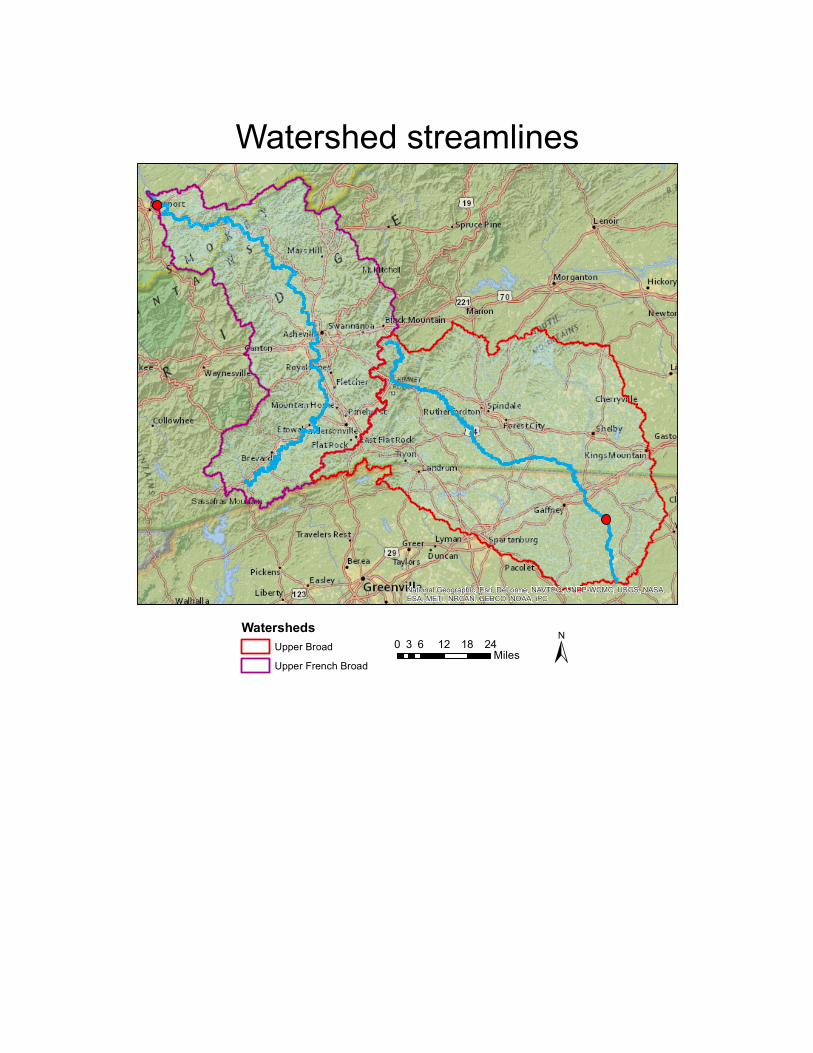
A  representative  stream  gage  was  also  located  in  each  watershed  in  order  to  

find  the  flow  rate  out  of  the  watershed.  The  gage  for  the  French  Broad  watershed  is  

located  very  close  to  the  outflow  point  to  the  next  watershed  and  should  provide  a  

good  approximation.  However,  the  gage  selected  for  the  Upper  Broad  River  

watershed  is  at  a  less  than  optimal  location  given  the  dearth  of  gages  within  this  

watershed.  The  locations  of  these  stream  gages  are  marked  with  red  dots  on  the  

following  maps.  

The  precipitation  and  streamflow  data  will  be  used  to  calculate  the  runoff  ratio  

–  the  fraction  of  runoff  that  becomes  streamflow  –  for  each  watershed.  

 

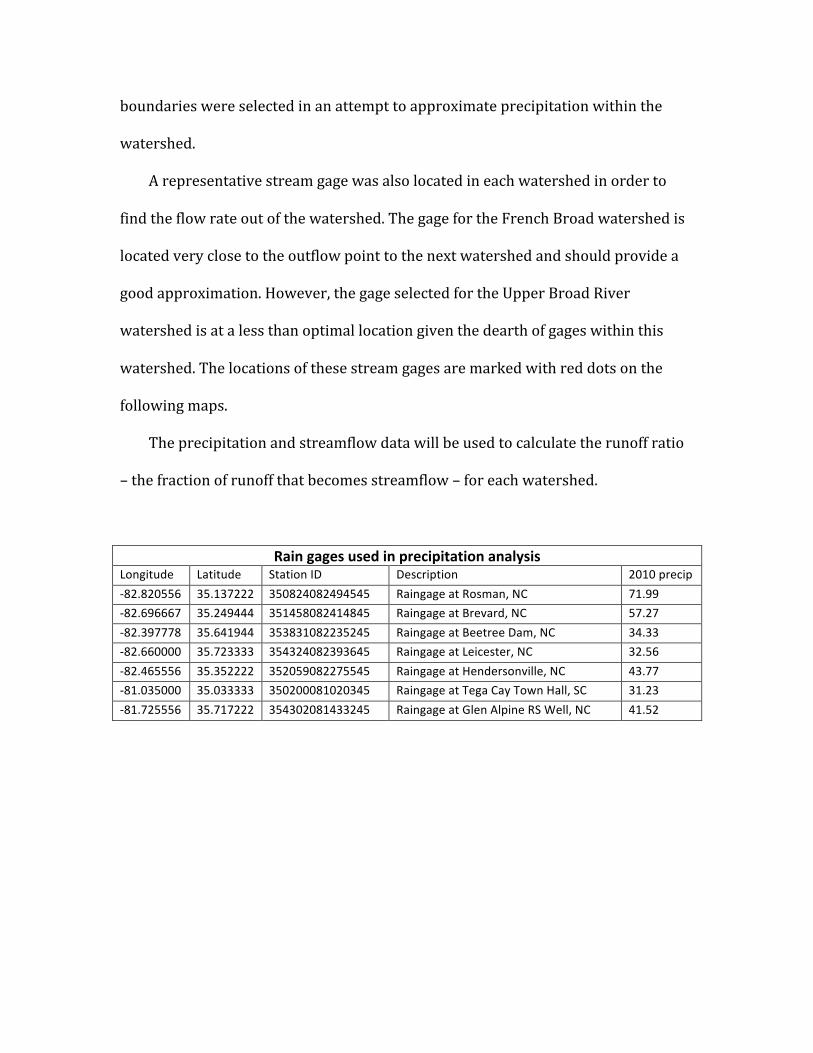
Rain  gages  used  in  precipitation  analysis  Longitude   Latitude   Station  ID   Description   2010  precip  -­‐82.820556   35.137222   350824082494545     Raingage  at  Rosman,  NC   71.99  -­‐82.696667   35.249444   351458082414845     Raingage  at  Brevard,  NC   57.27  -­‐82.397778   35.641944   353831082235245   Raingage  at  Beetree  Dam,  NC   34.33  -­‐82.660000   35.723333   354324082393645     Raingage  at  Leicester,  NC   32.56  -­‐82.465556   35.352222   352059082275545     Raingage  at  Hendersonville,  NC   43.77  -­‐81.035000   35.033333   350200081020345     Raingage  at  Tega  Cay  Town  Hall,  SC   31.23  -­‐81.725556   35.717222   354302081433245     Raingage  at  Glen  Alpine  RS  Well,  NC   41.52  

 

 

   

 

 

   The  nine  individual  1/9  arcsecond  DEMs  acquired  from  the  USGS  (above)  were  stitched  into  one  cohesive  DEM  (below)  using  the  Mosaic  to  New  Raster  tool  in  ArcGIS.  

   

Watershed elevations

0 6 12 18 243

Miles

WatershedsUpper Broad

Upper French Broad

Elevation (ft.)High : 1942

Low : 121±

   

National Geographic, Esri, DeLorme, NAVTEQ, UNEP-WCMC, USGS, NASA,

ESA, METI, NRCAN, GEBCO, NOAA, iPC

Watershed streamlines

0 6 12 18 243

Miles

WatershedsUpper Broad

Upper French Broad±

Data  analysis  

The  shape  of  a  hypsometric  curve  can  be  indicative  of  a  number  of  factors,  

including  changes  in  geomorphology  and  the  relative  age  of  such  features  (Perez-­‐

Pena  et  al.,  2009).  While  both  watersheds  exhibit  concave  hypsometric  curves,  the  

curve  for  the  Upper  Broad  River  is  extremely  concave,  since  most  of  the  land  within  

the  watershed  is  at  the  low  end  of  the  elevation  scale.  This  is  reflective  of  the  much  

more  even  terrain  of  the  watershed,  which  has  likely  experienced  more  weathering  

than  the  Upper  French  Broad  River  watershed.  

The  calculated  runoff  ratio  for  each  watershed  also  reflects  the  differing  

topography  between  the  two  areas.  Using  the  equation  

w  =  Q  /  P  

where  Q  is  long  term  streamflow  and  P  is  long  term  precipitation  (each  found  using  

the  aforementioned  methods),  the  runoff  ratio  for  the  Upper  French  Broad  River  

watershed  was  found  to  be  .449,  which  the  runoff  ration  for  the  Upper  Broad  River  

watershed  was  found  to  be  .293.  While  estimations  were  made  in  calculating  these  

ratios,  this  is  the  expected  result.  The  Upper  French  Broad  has  both  greater  

topography  overall  and  steeper  topography,  both  of  which  typically  generate  more  

runoff.  This  is  because  on  steeper  slopes,  it  is  more  difficult  for  water  to  infiltrate  

the  ground,  and  more  precipitation  finds  its  way  to  stream  channels.    

Given  these  factors,  the  Upper  French  Broad  River  watershed  is  likely  more  

prone  to  flooding  than  the  Upper  Broad  River  watershed.  

 

   

 

   

that hypsometric curve parameters have a pronouncedrelation with basin hydrology and particularly with itsflood response. Masek et al. (1994) proposed a climaticeffect in the hypsometry by comparing two large drainagebasins in the central Andean plateau. The differences inthese hypsometric curves reflected changes in erosionrates driven by climatic factors. Lifton and Chase (1992)studied the relations between tectonics and hypsometryin the San Gabriel Mountains, California. They found apositive correlation between uplift rate and the hypso-metric integral. In this study, they also proved alithological influence in the hypsometry at small scales(up to 100 km2). More recently, Chen et al. (2003) usedhypsometric integral values to differentiate betweendifferent morphotectonic provinces in the foothills ofTaiwan. Higher hypsometric integral values were relatedwith hanging walls of active thrusts with considerablevertical slip. These authors also tested the spatialinfluence in the hypsometry by comparing hypsometricintegral values in different basin types.

With the current development of geographical infor-mation systems (GIS), the calculation of hypsometriccurves has become easier. The spreading of digitalelevation models (DEMs) offers good raw material toanalyze hypsometry. It is not necessary to count on a verydetailed DEM, since the hypsometric curve is robustagainst variations in DEM resolution (Hurtrez et al.,1999; Keller and Pinter, 2002).

Luo (1998) proposed two methods to automaticallyextract hypsometric curves from digital contour maps andfrom DEM using the GIS architecture. In DEM, this authorproposed the use of zonal statistical functions integratedin GIS to obtain binned elevation frequencies from digitalelevation models.

In this paper, we present a method to extract relative-areas and relative elevations based on the raster

data-model from ArcGIS. We have developed an ArcGISextension (for ArcMap) termed CalHypso that allows theextraction of multiple hypsometric curves at once, as wellas the estimation of the statistical moments for eachcurve. To test this program, we have carried out ahypsometric analysis in the westernmost part of theSierra-Nevada dome (Betic Cordillera, South of Spain). Wehave obtained the hypsometric curves and the mainhypsometric statistics (Harlin, 1978; Luo, 2000) for theprincipal catchments in the north and south slope ofthe Sierra Nevada. The analysis suggests that the drainageevolution in this area is sensitive to the recent tectonics,thus reinforcing some ideas on the Neogene–Quaternaryevolution of the Sierra-Nevada dome.

2. Statistical moments of the hypsometric curve

Harlin (1978) developed a technique that treated thehypsometric curve as a cumulative probability distribu-tion and used its statistic moments to describe itquantitatively. This hypsometric technique has been usedto quantify hypsometric curve shapes with good results(Harlin, 1978; Luo, 2000, 2002). It consists the hypso-metric curve by a continuous polynomial function,(Harlin, 1978) (Fig. 1a)

f !x" # a0 $ a1x$ a2x2 $ % % % $ anxn. (1)

In this function f(x) values represent the relative-altitudes(h/H) and x values represent the relative-areas (a/A)(Fig. 1a). The relatively simple shape of the hypsometriccurve, generally with few inflexions, can be fitted to a low-order polynomial function of 2nd or 3rd grade (Harlin,1978). If we assume the hypsometric curve to be apolynomial function of 3rd grade of the form

f !x" # a0 $ a1x$ a2x2 $ a3x3. (2)

ARTICLE IN PRESS

Fig. 1. (a) Hypsometric curve after Strahler (1952). Area of region under curve (R) is known as hypsometric integral. Hypsometric curve can be representedby function f(x). Total elevation (H) is relief within basin (maximum elevation minus the minimum elevation), total area (A) is total surface area of basin,and area (a) is surface area within basin above a given altitude (h). (b) Changes in hypsometric curves (modified from Ohmori, 1993). Convex curves aretypical for youthful stages of maturity and s-shaped curves and concave curves for mature and old stages. Arrows indicate a direction of change in curvesaccording to the change in mountain altitude during a geomorphic cycle.

J.V. Perez-Pena et al. / Computers & Geosciences 35 (2009) 1214–1223 1215

An  explanation  of  what  the  different  shapes  of  hypsometric  curves  reflect.  Generally,  if  a  curve  has  a  convex  shape,  it  indicates  younger  geomorphology,  while  S-­‐shapes  and  concave  curves  indicate  greater  maturity.  (Perez-­‐Pena  et  al.,  2009)  

 

 

References  

Perez-­‐Pena,  J.V.;  J.M.  Azanon;  A.  Azor,  “CalHypso:  An  ArcGIS  extension  to  calculate  hypsometric  curves  and  their  statistical  moments.  Applications  to  drainage  basin  analysis  in  SE  Spain,”  2009,  Computers  &  Geosciences,  Vol.  35,  P.  1214-­‐1223.