eigenvector analysis of digital elevation models in a gis: geomorphometry … · ·...
TRANSCRIPT
199
Concepts and Modelling in Geomorphology: International Perspectives,Eds. I. S. Evans, R. Dikau, E. Tokunaga, H. Ohmori and M. Hirano, pp. 199–220.© by TERRAPUB, Tokyo, 2003.
Eigenvector Analysis of Digital Elevation Models in a GIS:Geomorphometry and Quality Control
Peter L. GUTH
Department of Oceanography, U.S. Naval Academy,Annapolis, Maryland 21402-5026, U.S.A.
e-mail: [email protected]
Abstract. Digital elevation models (DEMs) cover a wide range of scales, and allowstatisticalanalysis of geomorphometric parameters. At global or continental scale, DEMscovering rectangular quadrangles can be considered random samples. Average quadranglevalues can be compared at different DEM scales, and for different physiographicprovinces. Three independent variables provide valuable descriptions of terrain: averageelevation, average slope, and the degree of terrain organization. DEMs with spacings of30″ (global coverage), 3″ (continental United States), and 30 m (local United States)provide almost perfect correlations for average quadrangle elevation and slope, althoughthe slope values increase as the DEM spacing decreases. The degree of terrain organizationalso correlates across DEM scales, but with lower correlation coefficients, especially inareas of lower relief. Terrain variables computed from 10 m and 30 m USGS Level 2DEMs are essentially identical. Slope algorithms perform differently in differentphysiographic provinces, and the aspect algorithm performs poorly in low relief areas.Geomorphometric analysis can provide a rapid and effective assessment of DEM qualitycontrol, and should be integrated into the DEM production process.
Keywords: Digital-Elevation-Model, Geomorphometry, Slope-Algorithm, Aspect-Algorithm
INTRODUCTION
Digital elevations models (DEMs), rectangular grids of elevation values, providean unparalleled tool for geomorphometry. DEMs now cover a wide range ofscales, from global through continental and regional to local and almost pointscales. Analysis can extract a wide variety of parameters relating elevation, slope,aspect and terrain organization. Conversely, geomorphometry provides an idealtool for assessing the quality of DEMs. Outliers on histograms or bivariate plotsof geomorphometric parameters almost always represent flawed DEMs.
At small scales DEM data cover the entire world, but at large scale dataavailability reflects a bias toward the United States. This bias results from twofactors: (1) the United States government has one of the most aggressiveprograms in the world to produce DEMs, and (2) almost unique in the world, theUnited States national mapping agencies place no restrictions on their digitaldata. DEMs with 30 m spacing cover almost all of the United States, andincreasing numbers of 10 m DEMs are coming on line. With data spacing ranging
200 P. L. GUTH
from almost 10 km to 10 m, available DEMs span 4 orders of magnitude.Experimental 1 m resolution LIDAR (Light Detection and Ranging) DEMs coverareas almost point-like with vast quantities of data (NOAA Coastal Services DataCenter, 2001), and will add another order of magnitude to range of scales whenthey become widely available.
DATA
This study used DEMs from continental scale (30″ spacing, about 1 km),regional scale (3″ spacing, 60–90 m), and local scale (10–30 m spacing). Table1 summarizes the free data obtained from the www. These data sets will now fitcomfortably on hard disks of mainstream personal computers. All of these datasets use binary 2 byte elevations. The continental data sets are stored uncompressed,whereas the other data sets are stored with the same standard UNIX compressedfile structure obtained from the USGS web site. Because compression varies withthe type of terrain and the amount of smoothing from the DEM creation process,the estimates below should be viewed only as rough estimates for the order ofmagnitude of the DEM sizes. Further, if future large scale DEMs use 4 byte valuesfor elevation as the USGS is starting to implement, file sizes might double.
Three different United States government mapping agencies have createdquasi-independent continental 30″ DEMs: DTED Level 0 (NIMA, 2000), GLOBE(NOAA National Geophysical Data Center, 2001), and GTOPO30 (USGS EROSData Center, 2001). After downloading, the GLOBE and GTOPO30 datasetswere converted to 1° tiles to match the DTED, and provide a good statisticalsampling unit for comparisons. With 1° elevation tiles each data set will fit on asingle CD-ROM, if some of the interior cells in Antarctica are removed. Theflatness of the ice sheet and the convergence of the meridians make the 30″ DEMa poor choice for the polar regions.
The 250K DEM (USGS, 2001) was originally created by a precursor ofNIMA and contains many processing anomalies but remains a valuable regionaldata resource because of its availability. The current NIMA product, DTED Level1, provides a much better demonstration of what this data resolution can achievebut is unfortunately not publicly available. The DEMs used in this study cover allof the United States and Puerto Rico except for Alaska. The SRTM mission
Table 1. DEMs available for comparison.
Eigenvector Analysis of Digital Elevation Models in a GIS 201
should produce this world-wide data set for public use (Jet Propulsion Laboratory,2001), and the first samples covering some of the United States appeared in early2002 and South America in the summer of 2003. The SRTM data appeared too lateto include in this analysis, and will require careful consideration on how to handlethe data voids when conducting statistical analyses.
Over 51,000 24K DEMs were downloaded from the same USGS site alongwith the 250K DEM (USGS, 2001) in the summer of 2000, before the 24K DEMswere removed. USGS allowed an automated download process, the only practicalway to obtain such a large sample. This data, and an increasing number of 10 mDEMs, must now be downloaded free from two commercial sites that restrict thespeed or number of DEMs that can be, and which forbid the use of automated ftp,or in a reprojected format from the National Elevation Dataset (NED, Gesch andothers, 2002). While the data considered here have elevations stored as 2 byteintegers with foot or meter resolution, some newer DEMs now use 2 byte integerdecimeters and others use 4 byte floating point values.
The 24K DEMs have two characteristics relevant to a discussion ofgeomorphometry. The “Level” of the DEM assesses its quality: Level 1, no longerbeing produced, used profiling or similar photogrammetric methods to producelower quality DEMs, whereas the newer Level 2 DEMs used interpolation fromscanned contour lines (USGS National Mapping Division, 1997/1998). Exceptfor contour line “ghosts” where elevations corresponding to the source mapcontour lines are overrepresented in the DEM (Guth, 1999c), the Level 2 DEMsprovide a much better representation of the terrain. In addition, some DEMs haveboth 10 m and 30 m resolution. Ten meter resolution provides much greater visualdetail in representations of the terrain.
At 30 m spacing the data set includes 42,921 (80%) of the 53,873 24Kquadrangles in the continental United States, plus 81 DEMs in Puerto Rico andthe Virgin Islands, and provides an excellent sample for this scale data atcontinental resolution. Hawaiian data were not available on the USGS web site,and Alaska was not mapped at this scale. The SRTM mission (Jet PropulsionLaboratory, 2001) should produce this world-wide data set for US military use,although the radar’s smoothing might make the effective resolution lower thanthe nominal resolution. The data set includes about 1000 10 m level 2 DEMs, orabout 2% of the total area of the continental United States.
The following tests on the differences in calculated statistical parameterswill be conducted using these DEMs for geomorphometry:
1. How do the different 30″ continental DEMs differ?2. How do the 30″ continental and 3″ regional DEMs differ?3. How do the 3″ regional and 30 m local DEMs differ?4. How do the Level 1 and Level 2 local DEMs differ?5. How do the 10 m and 30 m Level 2 local DEMs differ?
GEOMORPHOMETRIC PARAMETERS
Pike (1988) introduced the concept of a geometric signature, a multi-variatedescription of topography using a suite of measures, and later expanded the
202 P. L. GUTH
concept with a listing of 49 variables that could be grouped into 22 attributes(Pike, 2001). He considered roughness and height the two most importantattributes, with two measures of texture in seventh and eleventh position. Fifteendifferent variables contribute to roughness.
This analysis will focus on three geomorphic parameters: average elevation,average slope, and organization strength. These parameters reflect the interactionof climate, lithology, and topography. Average elevation, combined with latitude,represents a primary control on climate for both precipitation and temperature.Slope depicts the ruggedness and dissection of the landscape. Organizationvalues measure the processes responsible for terrain formation; the most highlyorganized regions are in folded mountain belts or glacial drumlin fields. Averageelevation and average slope coincide with Pike’s (2001) most important attributes,but none of his experimental measures fully capture this organization parameter.
Computation of average slope requires selection of a slope algorithm; anumber have been proposed, and about a half dozen widely used (recent summariesin Skidinore, 1989; Guth, 1995; Hodgson, 1998; Jones, 1998). Results foraverage regional slope correlate very strongly among the various methods,although the absolute values vary. This analysis uses the steepest adjacentneighbor algorithm, but comparisons between the steepest adjacent neighbor andfour nearest neighbor methods show how the choice of slope method affectsgeomorphic results.
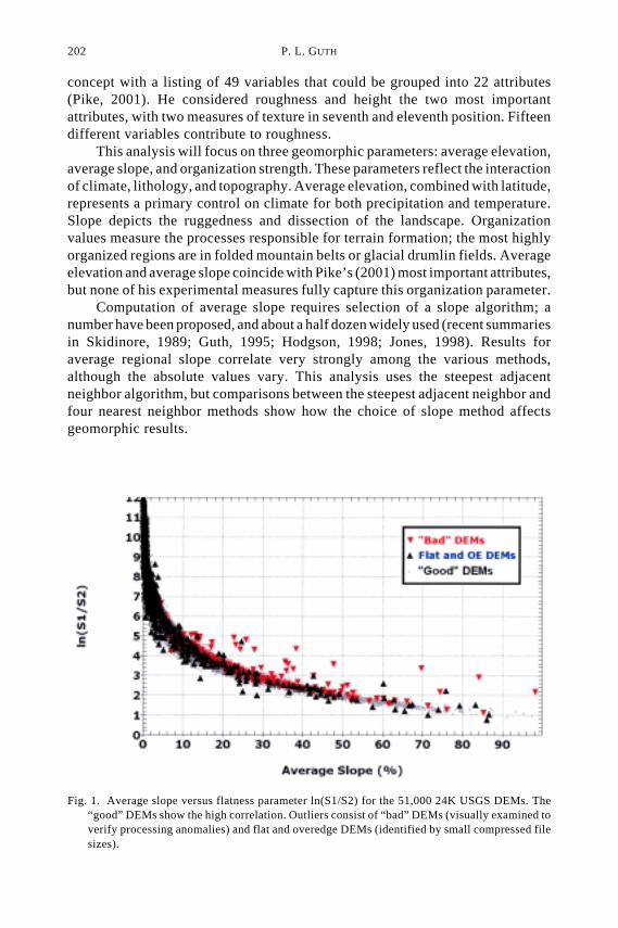
Fig. 1. Average slope versus flatness parameter ln(S1/S2) for the 51,000 24K USGS DEMs. The“good” DEMs show the high correlation. Outliers consist of “bad” DEMs (visually examined toverify processing anomalies) and flat and overedge DEMs (identified by small compressed filesizes).
Eigenvector Analysis of Digital Elevation Models in a GIS 203
Eigenvector methods can retrieve a flatness parameter and organizationparameter. Chapman (1952) proposed a graphical method using a stereo net tocharacterize terrain orientations. Woodcock (1977) described an eigenvaluemethod for fabric shapes in structural geology. The two methods can be combinedfor automatic characterization of terrain organization (Guth, 1999a, 1999b,2001). Direction consines of the landscape surface were computed from the slopeand aspect at each point, and then eigenvectors were obtained. The eigenvaluemethod extracts two independent parameters from the distribution of normals tothe earth’s surface calculated from the DEM, both logs of the ratios of eigenvalues.The ratio ln(Sl/S2) reflects a flatness parameter, and it correlates almost perfectlywith the average slope (Fig. 1). The correlation is negative because the log ratiois flatness and not steepness, and is not linear because of the log ratio. Thiscorrelation should not be surprising, since the eigenvalue method starts with theslope and aspect at each point and the orientation of the first eigenvector is theaverage normal to the earth’s surface.
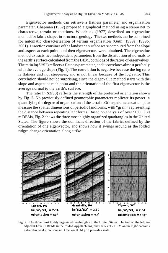
The ratio ln(S2/S3) reflects the strength of the preferred orientation shownby Fig. 2. No previously defined geomorphic parameters replicate its power inquantifying the degree of organization of the terrain. Other parameters attempt tomeasure the spatial dimensions of periodic landforms, with “grain” representingthe distance between repeating landforms. Based on analysis of over 50,000 30m DEMs, Fig. 2 shows the three most highly organized quadrangles in the UnitedStates. The figure shows the dominant direction of the fabric, defined by theorientation of one eigenvector, and shows how it swings around as the foldedridges change orientation along strike.
Fig. 2. The three most highly organized quadrangles in the United States. The two on the left areadjacent Level 1 DEMs in the folded Appalachians, and the level 2 DEM on the right containsa drumlin field in Wisconsin. One km UTM grid provides scale.
204 P. L. GUTH
Elevation is a true point parameter, defined at every grid location in theDEM. While slope is also a point parameter, it requires consideration of theneighboring elevations and various algorithms use from 2 to 8 adjacent neighbors.The most commonly used algorithm uses four neighbors and actually ignores theelevation of the central point to which the slope is assigned. The eigenvectormethod uses a region and probably requires at least 100 points for reasonablestatistical accuracy. While organization can be calculated as a point parameter fora particular region size about a point with a sliding window over the DEM (Guth,1999b, 2001), this study will concentrate of calculations with a 1° region size forglobal scale or 7 1/2′ region for continental scale. This quadrangle geomorphometryintroduces arbitrary aspects to the study, but sample sizes are large enough thatquadrangles represent reasonable sampling areas.
METHODS
All analyses used the MICRODEM program (Guth and others, 1987; Guth,1995). This program predates commercial GIS programs for personal computers,and while MICRODEM has now become a full-feature GIS program it retains agreater emphasis on DEMs and geomorphometry than any commercial program.While scripting within a GIS might duplicate the operations described here (e.g.contour line ghosts or terrain organization), I prefer embedding the capabilitieswithin MICRODEM where I have complete control of the operations anddisplays. With object-oriented programming, the DEM object contains methodsto calculate geomorphic parameters of the terrain.
MICRODEM indexes the DEMs, and sequentially processes them to calculategeomorphic parameters. For the 30″ global DEMs the program used 1° tiles. Forthe 3″ 250K DEM, the comparison used 1° tiles to compare with the 30″ data, and7 1/2′ tiles to compare with the 24K DEM. The program computed five variablesfor each tile: average slope, average elevation, the eigenvalue flatness andorganization parameters, and the direction of terrain organization. The databasecontains five additional fields for the DEM name and its bounding geographicrectangle. The program computed 28 additional parameters for the 24K DEM:duplicate variables to compare slope algorithms, DEM quality measures like theghost ratio (Guth, 1999c), and additional geomorphometric parameters whichwill not be discussed here but which could be used for a geometric signature(Pike, 2001).
The GIS database files for the geomorphic parameters allows summarystatistics, bivariate scatter plots, and map displays, with options to filter thedisplay—for example, to only show terrain organization for regions with greaterthan a specified average slope. The interactive nature of the GIS allows clickingon a point on the graph to show tabular data for that point and its location on themap. For the large data sets considered in this effort, the power of the GISrepresents the most effective way to explore the data.
Drawing on earlier work of Fenneman dating to 1917, the Fenneman andHoward (1946) map of the United States has 8 major divisions, 25 provinces, and86 sections representing distinctive areas having common topography, rock types
Eigenvector Analysis of Digital Elevation Models in a GIS 205
and structure, and geologic and geomorphic history. A digital version of the map(Hitt, 2002) was converted to geographic coordinates, and then each quadranglein the United States was assigned to the corresponding section. This allows theGIS to compute statistics based on the Fenneman physiographic regions.
Many of these analyses omit 24K DEMs identified as containing “bad” data,and those with a compressed file length less than 50 kb. Small file sizes occur intwo cases: coastal “overedge” DEMs where standard quadrangles leave a smallbit of land in what would be the next quadrangle, and extremely flat quadranglesin regions like the coastal plains. These DEMs account for a disproportionatenumber of the outliers on statistical plots. Overedge DEMs have an insufficientnumber of points for reliable statistics, and the DEMs do not have adequatevertical resolution for good statistics in very flat regions. The GIS also containsa percent ocean field for the global data sets; often the coastal DEMs should beignored for the eigenvector analysis. The 30″ 1° tiles contain only about 1400elevations, and when a significant proportion are missing the resulting statisticsrepresent outliers compared to full data sets.
SLOPE ALGORITHMS
While different slope algorithms correlate highly, they produce differentresults. Guth (1995) suggested using a steepest adjacent neighbor algorithm,while the most popular algorithm appears to be the four nearest neighbors (e.g.Hodgson, 1998; Jones, 1998), although Evans (1998) makes a convincing case forthe superiority of an eight neighbors algorithm. Because the steepest adjacentneighbor and four nearest neighbors have the greatest differences among thecommon methods, a detailed analysis of their differences highlights the effect ofslope algorithm on geomorphic parameters. Because slope and aspect provide theraw input to the eigenvector algorithm, the slope algorithm might affect theorganization calculations.
With an eight point neighborhood about the central point, eight partial slopescan be calculated in each of the eight principal cardinal directions. If the pointelevations are considered accurate, these represent the only unambiguous slopesthat can be determined. The challenge for the slope algorithm is to use thesevalues to estimate a single slope at the central point. The steepest adjacentneighbor algorithm uses the steepest of the eight slopes: this slope exists, it ismeasured over the DEM spacing (or the diagonal), and in many applications thesteepest slope is most important. The four nearest neighbors algorithm uses justfour neighbors: it is measured over twice the DEM spacing, and it smooths theresults by using twice the slope distance and not using the diagonal neighbors.
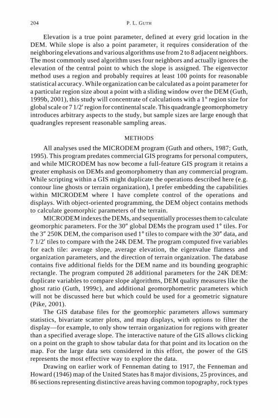
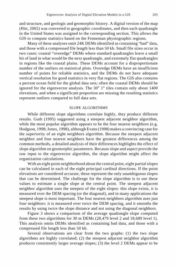
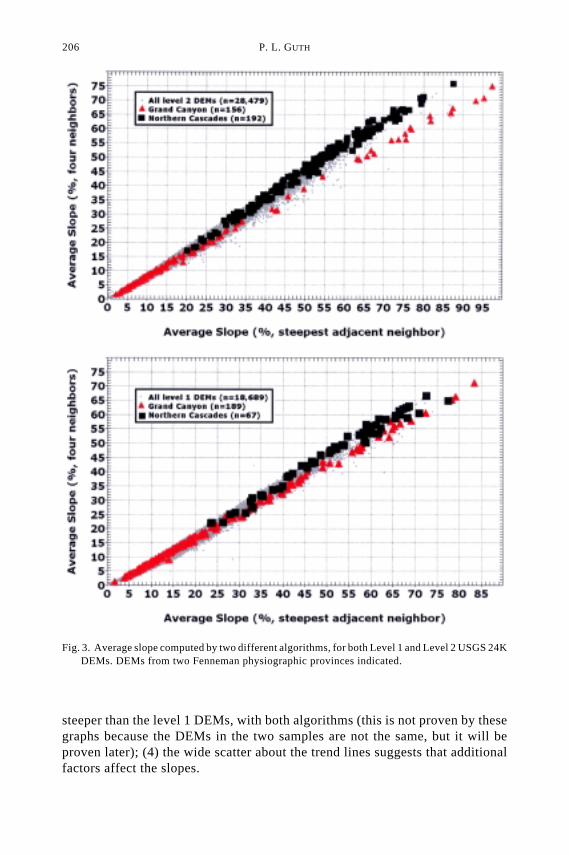
Figure 3 shows a comparison of the average quadrangle slope computedfrom these two algorithms for 30 m DEMs (28,479 level 2 and 18,689 level 1).This analysis omits DEMs identified as containing bad data, and those with acompressed file length less than 50 kb.
Several observations are clear from the two graphs: (1) the two slopealgorithms are highly correlated; (2) the steepest adjacent neighbor algorithmproduces consistently larger average slopes; (3) the level 2 DEMs appear to be
206 P. L. GUTH
steeper than the level 1 DEMs, with both algorithms (this is not proven by thesegraphs because the DEMs in the two samples are not the same, but it will beproven later); (4) the wide scatter about the trend lines suggests that additionalfactors affect the slopes.
Fig. 3. Average slope computed by two different algorithms, for both Level 1 and Level 2 USGS 24KDEMs. DEMs from two Fenneman physiographic provinces indicated.
Eigenvector Analysis of Digital Elevation Models in a GIS 207
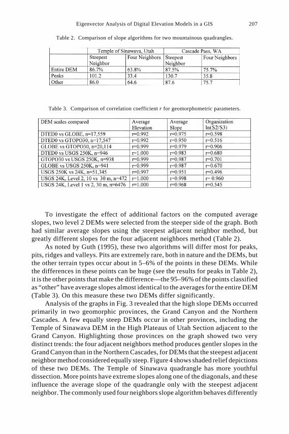
To investigate the effect of additional factors on the computed averageslopes, two level 2 DEMs were selected from the steeper side of the graph. Bothhad similar average slopes using the steepest adjacent neighbor method, butgreatly different slopes for the four adjacent neighbors method (Table 2).
As noted by Guth (1995), these two algorithms will differ most for peaks,pits, ridges and valleys. Pits are extremely rare, both in nature and the DEMs, butthe other terrain types occur about in 5–6% of the points in these DEMs. Whilethe differences in these points can be huge (see the results for peaks in Table 2),it is the other points that make the difference—the 95–96% of the points classifiedas “other” have average slopes almost identical to the averages for the entire DEM(Table 3). On this measure these two DEMs differ significantly.
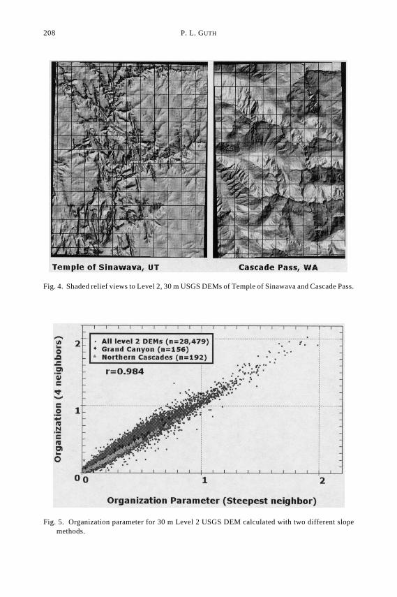
Analysis of the graphs in Fig. 3 revealed that the high slope DEMs occurredprimarily in two geomorphic provinces, the Grand Canyon and the NorthernCascades. A few equally steep DEMs occur in other provinces, including theTemple of Sinawava DEM in the High Plateaus of Utah Section adjacent to theGrand Canyon. Highlighting those provinces on the graph showed two verydistinct trends: the four adjacent neighbors method produces gentler slopes in theGrand Canyon than in the Northern Cascades, for DEMs that the steepest adjacentneighbor method considered equally steep. Figure 4 shows shaded relief depictionsof these two DEMs. The Temple of Sinawava quadrangle has more youthfuldissection. More points have extreme slopes along one of the diagonals, and theseinfluence the average slope of the quadrangle only with the steepest adjacentneighbor. The commonly used four neighbors slope algorithm behaves differently
Table 2. Comparison of slope algorithms for two mountainous quadrangles.
Table 3. Comparison of correlation coefficient r for geomorphometric parameters.
208 P. L. GUTH
Fig. 4. Shaded relief views to Level 2, 30 m USGS DEMs of Temple of Sinawava and Cascade Pass.
Fig. 5. Organization parameter for 30 m Level 2 USGS DEM calculated with two different slopemethods.
Eigenvector Analysis of Digital Elevation Models in a GIS 209
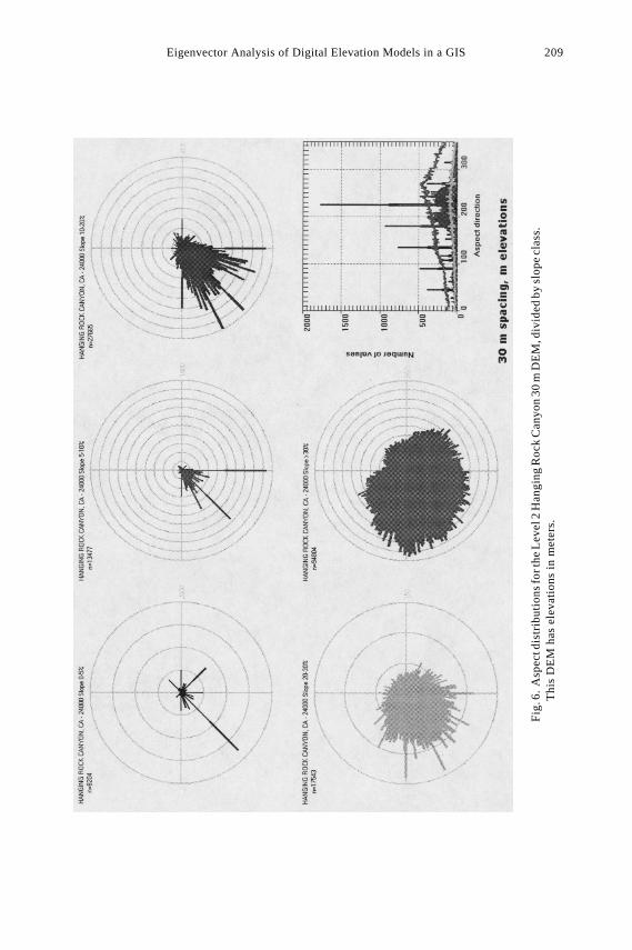
Fig
. 6.
Asp
ect d
istr
ibut
ions
for t
he L
e ve l
2 H
a ngi
ng R
ock
Can
yon
30 m
DE
M, d
ivid
ed b
y sl
ope
c la s
s.T
his
DE
M h
a s e
leva
tion
s in
me t
e rs.
210 P. L. GUTH
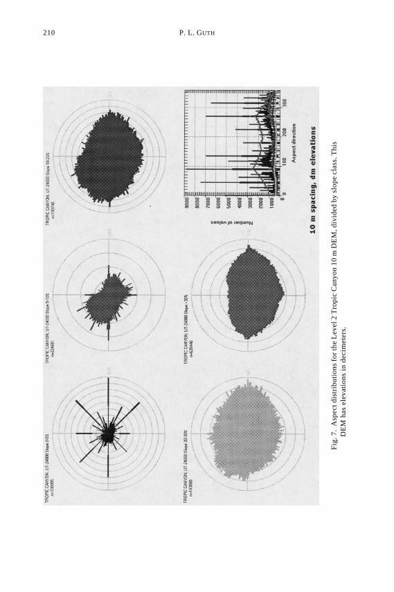
Fig
. 7.
Asp
ect d
istr
ibut
ions
for
the
Le v
e l 2
Tro
pic
Ca n
yon
10 m
DE
M, d
ivid
ed b
y sl
ope
c la s
s. T
his
DE
M h
a s e
leva
tion
s in
de c
ime t
e rs.
Eigenvector Analysis of Digital Elevation Models in a GIS 211
in different physiographic provinces, compared to the steepest adjacent neighboralgorithm.
Since the eigenvector technique relies on the slope as input, Fig. 5 shows theorganization parameter for level 2 DEMs calculated with the two slope algorithms.Scatter is minimal, the graph’s slope is close to 1, and the differences do notcorrelate with the physiographic province. The eigenvector technique appears toextract organization independent of the slope algorithm use.
ASPECT ALGORITHM
Selection of an aspect algorithm presents much less choice than that of aslope algorithm, because extending many of the slope algorithms would result ina very limited number of possible aspect directions. Guth (1995) suggested useof the eight nearest neighbors with even weighting, and that algorithm has beenused here. However, this algorithm does not provide an even or uniform distributionof aspects.
Figure 6 shows the aspects for a 30 m DEM. Note the spikes in the aspectdistribution, especially prominent for the low slope parts of the DEM. Aspects at45° intervals are overrepresented, and the algorithm appears to work well onlywhen the slope exceeds 30%. The problem originates in the discrete nature of theelevations: with meter elevation resolution and 30 m spacing, the basic slopevalues only change by 1/30. To verify this assumption, Fig. 7 shows the aspectdistributions for a 10 m DEM with elevations in decimeters. This allows slopevalues to change by 1/100, and in this case the algorithm appears to produceuniform and natural aspect distributions if the slope is steeper than 10%.
RESULTS
Table 3 summarizes the results of the comparisons of DEMs at differentscales or sources. The correlation coefficients for both average slope and averageelevation exceed 0.95 for all the comparisons, but with these sample sizes suchcorrelation coefficients still allow some scatter and some significant anomalies.The organization parameter shows more scatter and lower correlations.
1. Continental data sets
The continental data sets agree with each other extremely well for averageslope and average elevation, and less well for organization level. Table 3 showscorrelation coefficients greater than 0.99 for elevation and 0.95 for slope, and aslow as 0.51 for organization. GTOPO30 and GLOBE show the strongestcorrelation, and both have complete coverage of the world. DTED level 0 does notinclude Antarctica, and still has a large gap in the Amazon Basin.
Despite correlation coefficients for average elevation exceeding 0.99,differences in average elevation for 1° cells can exceed 2000 m. Six cells in theAndes of Peru and Bolivia have differences this large between DTED andGLOBE, and one has a difference exceeding 3000 m. This suggests that for partsof the world the continental data sets still have significant problems.
212 P. L. GUTH
Fig
. 8.
C
ompa
riso
n of
the
org
a niz
a tio
n pa
ram
e te r
ln(
S2/
S3)
ca l
c ula
ted
from
DT
ED
Lev
e l 0
and
GL
OB
E f
or 1
° c e
lls.
Not
e th
a t (
a ) h
a s a
dif
fere
nt s
c ale
tha
n th
e ot
hers
.
Eigenvector Analysis of Digital Elevation Models in a GIS 213
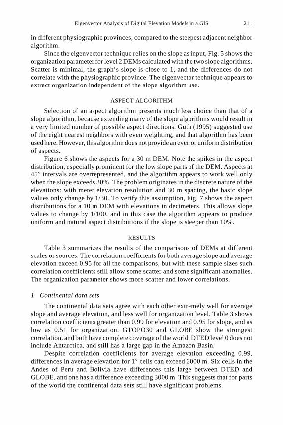
To investigate how well the continental data sets work in regions with gooddigital representations of topography, Fig. 8 shows the scatter plots for organizationplotted from DTED and GLOBE. Figure 8a shows the global data, with a greatdeal of scatter and a correlation of 0.594. With the data restricted to part of NorthAmerica (N23–N54, and W130–W73), Fig. 8b shows much less scatter and animproved correlation of 0.887. Restricting the data to regions with slopes greaterthan 2% and 5% in Figs. 8c and 8d increases the correlation even further to 0.97.Organization values have the least reliability in regions of low slope.
Assessing the accuracy of DTED Level 0 versus GLOBE or GTOPO30remains beyond the scope of this work, because it likely varies regionally. Thetremendous differences in average elevation noted above occur on the easternflank of the Andes, where DTED shows the average elevation in one cell to beover 2000 m higher than the cell immediately to the east, and neighboring cellsdo not even remotely match along their common edge. Only a few of the cells inthat region used higher resolution DTED as their source, and most of the othersshow only the grossest outlines of topography. GTOPO30 and GLOBE improvethe elevation picture somewhat in that region, but clearly show which cells hadhigh resolution source data available. The SRTM 30″ global set has just beenreleased (summer 2003), and should now be used for this scale analysis.
2. Continental versus regional DEMs
This comparison must be restricted to the United States because of the lackof publicly available data elsewhere. Table 3 shows the comparison of about 940
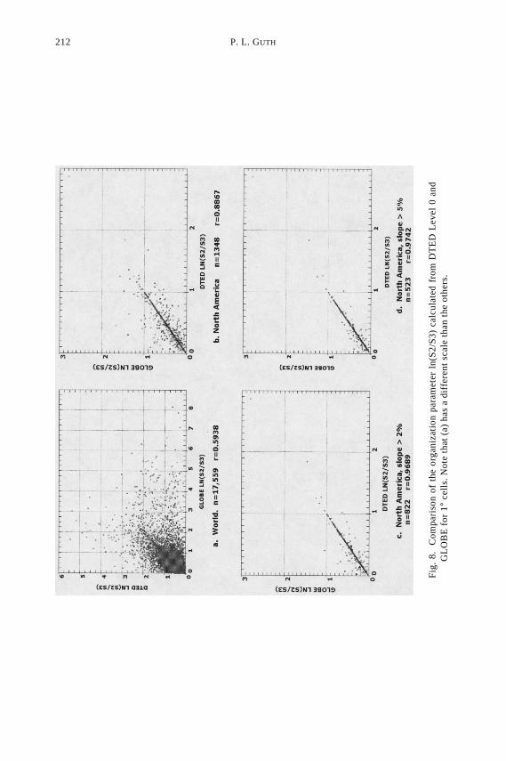
Fig. 9. Comparison of the organization parameter between DTED 0 and the USGS 3″ , 250K DEM.This shows the 432 cells covering the United States with an average slope in the USGS DEMgreater than 5%.
214 P. L. GUTH
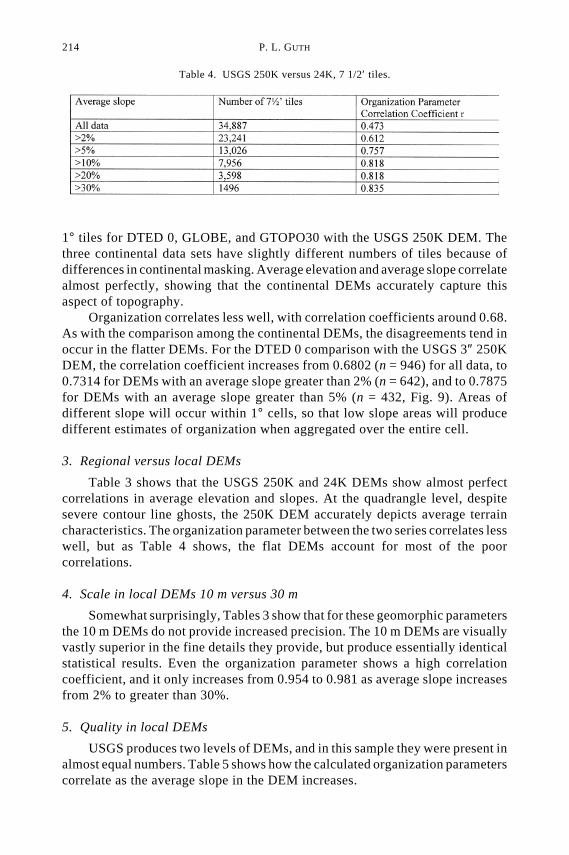
1° tiles for DTED 0, GLOBE, and GTOPO30 with the USGS 250K DEM. Thethree continental data sets have slightly different numbers of tiles because ofdifferences in continental masking. Average elevation and average slope correlatealmost perfectly, showing that the continental DEMs accurately capture thisaspect of topography.
Organization correlates less well, with correlation coefficients around 0.68.As with the comparison among the continental DEMs, the disagreements tend inoccur in the flatter DEMs. For the DTED 0 comparison with the USGS 3″ 250KDEM, the correlation coefficient increases from 0.6802 (n = 946) for all data, to0.7314 for DEMs with an average slope greater than 2% (n = 642), and to 0.7875for DEMs with an average slope greater than 5% (n = 432, Fig. 9). Areas ofdifferent slope will occur within 1° cells, so that low slope areas will producedifferent estimates of organization when aggregated over the entire cell.
3. Regional versus local DEMs
Table 3 shows that the USGS 250K and 24K DEMs show almost perfectcorrelations in average elevation and slopes. At the quadrangle level, despitesevere contour line ghosts, the 250K DEM accurately depicts average terraincharacteristics. The organization parameter between the two series correlates lesswell, but as Table 4 shows, the flat DEMs account for most of the poorcorrelations.
4. Scale in local DEMs 10 m versus 30 m
Somewhat surprisingly, Tables 3 show that for these geomorphic parametersthe 10 m DEMs do not provide increased precision. The 10 m DEMs are visuallyvastly superior in the fine details they provide, but produce essentially identicalstatistical results. Even the organization parameter shows a high correlationcoefficient, and it only increases from 0.954 to 0.981 as average slope increasesfrom 2% to greater than 30%.
5. Quality in local DEMs
USGS produces two levels of DEMs, and in this sample they were present inalmost equal numbers. Table 5 shows how the calculated organization parameterscorrelate as the average slope in the DEM increases.
Table 4. USGS 250K versus 24K, 7 1/2′ tiles.
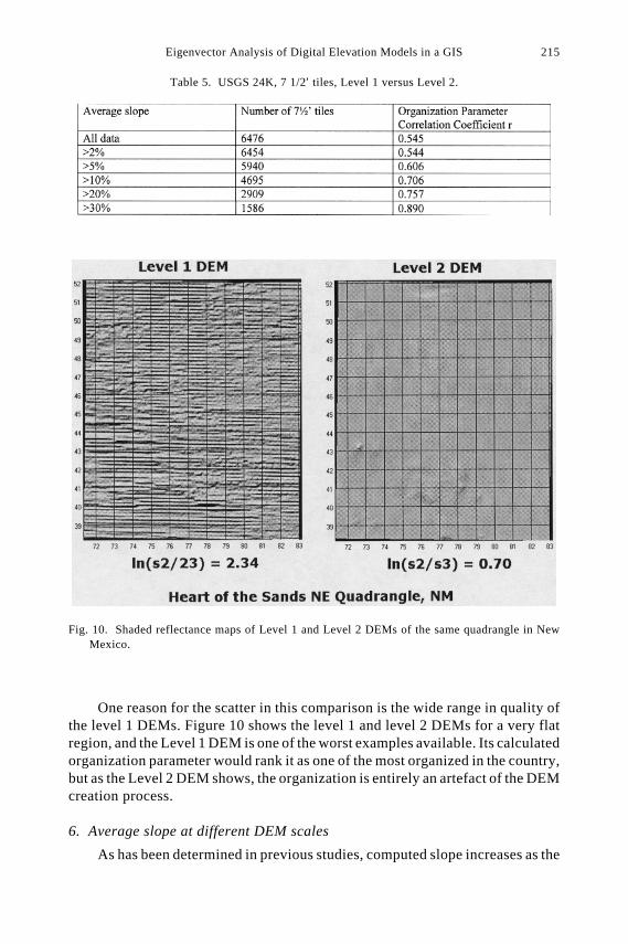
Eigenvector Analysis of Digital Elevation Models in a GIS 215
One reason for the scatter in this comparison is the wide range in quality ofthe level 1 DEMs. Figure 10 shows the level 1 and level 2 DEMs for a very flatregion, and the Level 1 DEM is one of the worst examples available. Its calculatedorganization parameter would rank it as one of the most organized in the country,but as the Level 2 DEM shows, the organization is entirely an artefact of the DEMcreation process.
6. Average slope at different DEM scales
As has been determined in previous studies, computed slope increases as the
Fig. 10. Shaded reflectance maps of Level 1 and Level 2 DEMs of the same quadrangle in NewMexico.
Table 5. USGS 24K, 7 1/2′ tiles, Level 1 versus Level 2.
216 P. L. GUTH
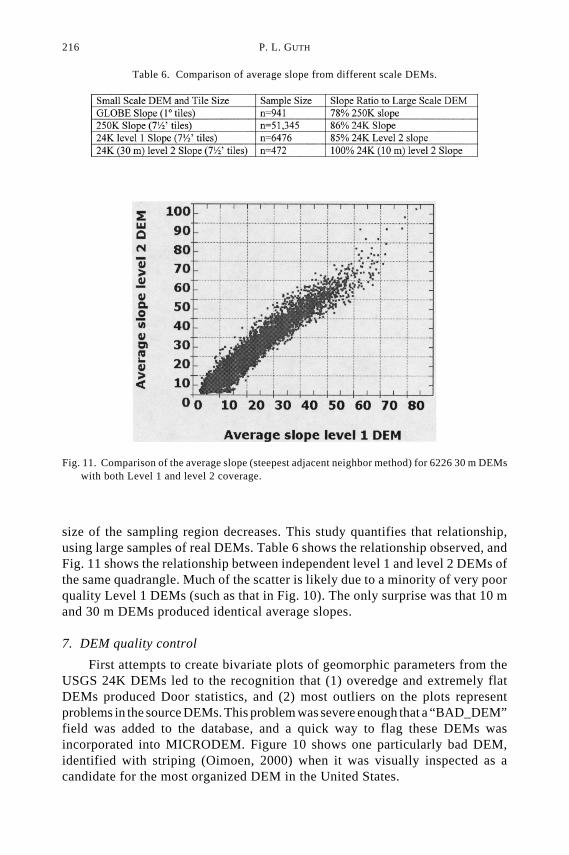
size of the sampling region decreases. This study quantifies that relationship,using large samples of real DEMs. Table 6 shows the relationship observed, andFig. 11 shows the relationship between independent level 1 and level 2 DEMs ofthe same quadrangle. Much of the scatter is likely due to a minority of very poorquality Level 1 DEMs (such as that in Fig. 10). The only surprise was that 10 mand 30 m DEMs produced identical average slopes.
7. DEM quality control
First attempts to create bivariate plots of geomorphic parameters from theUSGS 24K DEMs led to the recognition that (1) overedge and extremely flatDEMs produced Door statistics, and (2) most outliers on the plots representproblems in the source DEMs. This problem was severe enough that a “BAD_DEM”field was added to the database, and a quick way to flag these DEMs wasincorporated into MICRODEM. Figure 10 shows one particularly bad DEM,identified with striping (Oimoen, 2000) when it was visually inspected as acandidate for the most organized DEM in the United States.
Table 6. Comparison of average slope from different scale DEMs.
Fig. 11. Comparison of the average slope (steepest adjacent neighbor method) for 6226 30 m DEMswith both Level 1 and level 2 coverage.
Eigenvector Analysis of Digital Elevation Models in a GIS 217
Average quadrangle slope initially revealed the most defective DEMs,because the bad elevations are usually so much larger than the others that theyaffect the average. Figure 1 shows the strong relationship between averagequadrangle slope and the flatness parameter. After first flagging flat and overedgeDEMs, a number of outliers remained. These had a higher average slope than theirflatness parameter would indicate. Clicking the point on the graph brings up thedatabase table for that record, and a click there opens the DEM. When visualanalysis confirms that the DEM is defective, it can be flagged and ignored forfurther analysis. This pair of variables works because bad values affect thearithmetic mean used for average slope more than they affect the vector averageused for the flatness parameter.
The following errors have been identified: (1) large rectangular regions ofthe DEM with uniform, erroneous elevations (probably a flag representingregions of no data, appropriate to processing software but not to the SDTS DEMprofile); (2) a single partial row or column of bad elevations along one margin ofthe DEM (often one or two bad postings); (3) a single spike elevation, in somecases where a posting in feet was inserted into a DEM in meters; (4) snaking“lines” of bad elevations within the DEM; (5) DEMs mislabeled as feet or metersinstead of the correct value, which show up in regional maps of average elevationwhere they are either three times or one third the elevation of their neighbors; (6)lakes with a uniform elevation that does not match the surroundings, or the heighton the topographic map. The striping artefacts in some level 1 DEMs (Oimoen,2000) are not included, because I have not been able to automate their identification,and assessing their severity remains a very subjective process.
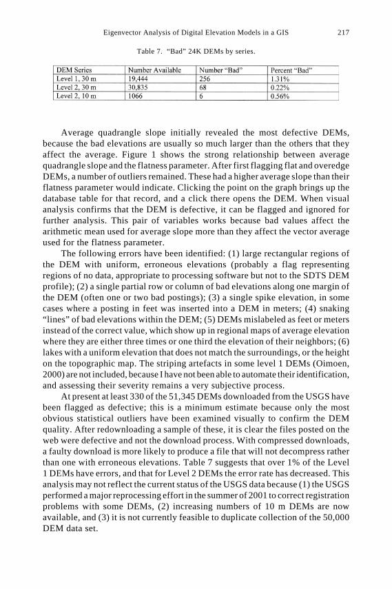
At present at least 330 of the 51,345 DEMs downloaded from the USGS havebeen flagged as defective; this is a minimum estimate because only the mostobvious statistical outliers have been examined visually to confirm the DEMquality. After redownloading a sample of these, it is clear the files posted on theweb were defective and not the download process. With compressed downloads,a faulty download is more likely to produce a file that will not decompress ratherthan one with erroneous elevations. Table 7 suggests that over 1% of the Level1 DEMs have errors, and that for Level 2 DEMs the error rate has decreased. Thisanalysis may not reflect the current status of the USGS data because (1) the USGSperformed a major reprocessing effort in the summer of 2001 to correct registrationproblems with some DEMs, (2) increasing numbers of 10 m DEMs are nowavailable, and (3) it is not currently feasible to duplicate collection of the 50,000DEM data set.
Table 7. “Bad” 24K DEMs by series.
218 P. L. GUTH
Maximum point slope is probably the single best parameter for flagging badDEMs. While a few DEMs have valid huge point slopes, like the volcanic neckat Ship Rock, New Mexico (slope 1561%) or the cliff face of Half Dome inYosemite National Park (slope 1553%), excessive point slope values over 1000%almost always represent bad postings in the DEM (at least 291 of 364 bad DEMsin this sample). While many of the errors in these DEMs are not severe and wouldnot significantly affect most uses of the DEM, they could be eliminated with asimple quality control step. The DEM should be displayed as a shaded reflectancemap, the location of the steepest point slope flagged, and the elevations of thepostings surrounding the point displayed. The maximum slope could be comparedto the distribution of maximum slope with the Fenneman province, and if themaximum slope in the DEM occurs in a pit, the point almost certainly representsan error. The DEM could then be accepted, or additional edits performed. Whilethis sample was downloaded in the summer of 2000, some of the bad DEMs arestill present on the commercial servers now distributing the USGS data. Osbornand others (2001) describe the challenges faced by USGS in developing qualitycontrol methods for the DEMs.
CONCLUSIONS
• Different slope algorithms behave differently depending on thephysiographic province. Most of the difference between the steepest adjacentneighbor algorithm and the four nearest neighbors algorithms is not due to thesmall number of peaks, ridges, and valleys, which can have huge differences, butto the vast majority of points which cannot easily be categorized over a nine pointregion.
• Aspect algorithms do not work well in low relief regions, producing toomany aspects at 45° intervals. They never work well at very low slopes, and thesteepness at which they begin to produce uniform results appears to be related tothe ratio of vertical resolution to horizontal resolution in the DEM.
• Different scales of DEMs accurately capture average elevation, whichcorrelates very strongly across scales.
• Different scales of DEMs accurately capture average slope, whichcorrelates very strongly across scales. The absolute value of average slopeincreases as the resolution of the DEM increases (post spacing decreases),although there appears to be no change between data spacings of 10 and 30 m.
• Different scales of DEMs accurately capture terrain organization, bothin orientation and magnitude. The correlation is weakest in low slope regions,probably because of problems with the aspect algorithms, and is strongest inmoderate to high relief areas.
• Geomorphic parameters can provide quality control for DEMs.Experience with the USGS DEMs suggests that a simple maximum point slopecheck should be performed on all DEMs, with excessive values over 1000%almost always representing bad postings in the DEM. This procedure should beimplemented in the DEM production process.
Eigenvector Analysis of Digital Elevation Models in a GIS 219
Acknowledgements—I thank Richard Pike for his roles in organizing the Tokyo symposium,inviting me to attend, and generally encouraging me to pursue this work. The openness ofU.S. government mapping agencies in sharing digital data on the web made this workpossible, because without huge samples of free data this analysis would not have beenpossible.
REFERENCES
Chapman, C. A. (1952) A new quantitative method of topographic analysis: American Journal ofScience, 250, 428–452.
Evans, I. S. (1998) What do terrain statistics really mean?: In S. N. Lane, K. S. Richards and J. H.Chandler (eds.), Landform Monitoring, Modelling and Analysis, Ch. 6, pp. 119–138. J. Wiley,Chichester.
Fenneman, N. M. and Johnson, D. W. (1946) Physical divisions of the United States: United StatesGeological Survey, Map, Scale 1:7,000,000.
Gesch, D. B., Oimoen, M., Greenlee, S., Nelson, C., Steuck, M. and Tyler, D. (2002) The nationalelevation dataset: Photogrammetric Engineering & Remote Sensing, 68, 5–11.
Guth, P. L. (1995) Slope and aspect calculations on gridded digital elevation models: Examples froma geomorphometric toolbox for personal computers: Zeitschrift für Geomorphologie N.F.,Supplementband, 101, 31–52.
Guth, P. L. (1999a) Quantifying topographic fabric: eigenvector analysis using digital elevationmodels: In R. J. Merisko (ed.), 27th Applied Imagery Pattern Recognition (AIPR) Workshop:Advances in Computer-Assisted Recognition, 14–16 Oct. 1988, Washington, D.C., Proceedingsof SPIE [The International Society for Optical Engineering], Vol. 3584, pp. 233–243.
Guth, P. L. (1999b) Quantifying and visualizing terrain fabric from digital elevation models: In J.Diaz, R. Tynes, D. Caldwell and J. Ehlen (eds.), Geocomputation 99: Proceedings of the 4thInternational Conference on GeoComputation, Fredericksburg, Virginia, USA, 25–28 July,1999, CD-ROM ISBN 0-9533477-1-0. Available online at http://www.geovista.psu.edu/geocomp/geocomp99/index.htm
Guth, P. L. (1999c) Contour line “ghosts” in USGS Level 2 DEMs: Photogrammetric Engineering& Remote Sensing, 65, 289–296.
Guth, P. L. (2001) Quantifying terrain fabric in digital elevation models: In J. Ehlen and R. S.Harmon (eds.), The Environmental Legacy of Military Operations, 14, Chapter 3. GeologicalSociety of America Reviews in Engineering Geology.
Guth, P. L., Ressler, E. K. and Bacastow, T. S. (1987) Microcomputer program for manipulatinglarge digital terrain models: Computers & Geosciences, 13, 209–213.
Hitt, K. J. (2002) Metadata for physical divisions of the United States, digital version of Fennemanmap: http://water.usgs.gov/GIS/metadata/usgswrd/physio.html
Hodgson, M. E. (1998) Comparison of angles from surface slope/aspect algorithms: Cartographyand Geographic Information Systems, 25, 173–185.
Jet Propulsion Laboratory (2001) Shuttle Radar Topography Mission: http://www.jpl.nasa.gov/srtm/ (last update on page listed as 12/6/2001, accessed 1/3/2002).
Jones, K. H. (1998) A comparison of algorithms used to compute hill slope as a property of the DEM:Computers & Geosciences, 24, 315–324.
NIMA (2000) Geospatial Engine: http://164.214.2.59/geospatial/digital_products.htm (last updateon page listed as 12/14/2000, accessed 12/22/2001).
NOAA Coastal Services Data Center (2001) Topographic change mapping: http://www.csc.noaa.gov/crs/tcm/index.html (last update on page listed as 12/14/2000, accessed 12/22/2001).
NOAA National Geophysical Data Center (2001) The Global Land One-km Base Elevation(GLOBE) Project: Get GLOBE Data: http://www.ngdc.noaa.gov/seg/topo/globeget.shtml (lastupdate on page listed as 2/27/2001, accessed 12/22/2001).
Oimoen, M. J. (2000) An effective filter for removal of production artifacts in U.S. GeologicalSurvey 7.5-minute digital elevation models: Proceedings of the 14th International Conference,Applied Geologic Remote Sensing, 6–8 November 2000, Las Vegas, Nevada, pp. 311–319.

220 P. L. GUTH
Osborn, K., List, J., Gesch, D., Crowe, J., Merrill, G., Constance, E., Mauck, J., Lund, C., Caruso,V. and Kosovich, J. (2001) National digital elevation program (NDEP): In D. F. Maune (ed.),Digital Elevation Model Technologies and Applications: The DEM Users Manual, pp. 83–120.American Society for Photogrammetry and Remote Sensing, Bethesda, MD.
Pike, R. J. (1988) The geometric signature: quantifying landslide-terrain types from digital elevationmodels: Mathematical Geology, 20, 491–512.
Pike, R. J. (2001) Geometric signatures-experimental design, first results: In H. Ohmori (ed.), DEMsand Geomorphometry, Special Publications of the Geographic Information Systems Association,Proceedings of the symposia on New Concepts and Modeling in Geomorphology andGeomorphometry, DEMs and GIS, held 24–26 August, 2001, Tokyo, Fifth InternationalConference on Geomorphology, 1, pp. 50–51.
Skidmore, A. K. (1989) A comparison of techniques for calculating gradient and aspect from agridded digital elevation model: International Journal of Geographical Information Systems, 3,323–334.
USGS EROS Data Center (2001) GTOPO30, Global Topographic Data: http://edcdaac.usgs.gov/gtopo30/gtopo30.html (last update on page listed as 7/19/2001, accessed 12/22/2001).
USGS (2001) USGS Geographic Data Download: http://edcwww.cr.usgs.gov/doc/edchome/ndcdb/ndcdb.html (last update on page listed as 10/29/2001, accessed 12/22/2001).
USGS National Mapping Division (1997/1998) Standards for digital elevation models: http://rockyweb.cr.usgs.gov/nmpstds/demstds.html
Woodcock, N. H. (1977) Specification of fabric shapes using an eigenvalue method: GeologicalSociety of America Bulletin, 88, 1231–1236.