geometry and performance of timber gridshells naicu, dragos

University of Bath

MPHIL

Geometry and Performance of Timber Gridshells

Naicu, Dragos

Award date:2012

Awarding institution:University of Bath

Link to publication

Alternative formatsIf you require this document in an alternative format, please contact:[email protected]

Copyright of this thesis rests with the author. Access is subject to the above licence, if given. If no licence is specified above,original content in this thesis is licensed under the terms of the Creative Commons Attribution-NonCommercial 4.0International (CC BY-NC-ND 4.0) Licence (https://creativecommons.org/licenses/by-nc-nd/4.0/). Any third-party copyrightmaterial present remains the property of its respective owner(s) and is licensed under its existing terms.

Take down policyIf you consider content within Bath's Research Portal to be in breach of UK law, please contact: [email protected] with the details.Your claim will be investigated and, where appropriate, the item will be removed from public view as soon as possible.

Download date: 11. Mar. 2022

https://researchportal.bath.ac.uk/en/studentthesis/geometry-and-performance-of-timber-gridshells(315b37eb-fe04-4268-a00f-c19d7d41c696).html

Geometry and Performance of Timber Gridshells

By Dragos-Iulian Naicu

Supervised by

Dr. Chris Williams

Prof. Richard Harris

A thesis submitted for the degree of Master of Philosophy

The University of Bath

Department of Architecture and Civil Engineering

October 2012

Attention is drawn to the fact that copyright of this thesis rests with its author. A copy of this thesis

has been supplied on condition that anyone who consults it is understood to recognise that its

copyright rests with the author and they must not copy it or use material from it except as permitted

by law or with the consent of the author.

This thesis may be made available for consultation within the University Library and may be

photocopied or lent to other libraries for the purposes of consultation.

3

Acknowledgements

I would like to express my sincere gratitude towards my supervisors Dr. Chris Williams and Prof.

Richard Harris for their invaluable guidance, support and inspiration. I must thank my mother and

father for supporting me every step of the way and always reminding me to aim high. Also, to my

friends and colleagues in the department, specifically to Daniel Brandon for sharing his mechanics

expertise and to Daniel Gebreiter for our many side-topic conversations.

5

Abstract

Timber gridshells are a very efficient way of covering large spaces while also providing a unique

architectural and material quality. As this can still be considered an emergent technology, the design

of such buildings has relied on a relatively substantial amount of experimental work.

This thesis, upon reviewing the design and construction processes of previous timber gridshells, puts

forward a structural model that aims to represent the true nature and specifics of single and double-

layered timber gridshells. The parametrically determined geometry of a computational prototype is

described and used as a basis for a non-linear elastic numerical analysis.

Particular attention is given to modelling the connections between the timber laths that provide

composite bending action in a double layer grid. The deformation behaviour and the imperfection

sensitivity are assessed with a view to understanding how gridshells respond under different

conditions.

A new gridshell will inevitably be analysed with computer software, but the information presented in

this dissertation will be useful for scheme design as well as the calibration of the computer analysis.

7

List of Figures

Figure 1. 1 Pantheon, Rome; engraving (Jombert, 1779) ..................................................................... 18

Figure 1. 2 Discrete steel member gridshells. Top: British Museum Great Court Roof. Bottom:

Smithsonian American Art Museum (Architects’ Journal) .................................................................... 19

Figure 1. 3 Discrete timber member gridshell. Pods Sports Complex (S&P Architects) ....................... 20

Figure 1. 4 Forces in continuous and lattice shells ............................................................................... 21

Figure 1. 5 Funicular and disturbing loads ............................................................................................ 21

Figure 1. 6 Single-layered and Double-layered timber gridshell element ............................................ 22

Figure 1. 7 Types of bracing systems .................................................................................................... 23

Figure 1. 8 Plan and Section of Double-layered timber gridshell element. (Harris et al., 2003a) p28 . 23

Figure 1. 9 Connection detail. Left: Slotted hole connection. Middle: Pattented nodal connection.

Right: Pattented nodal connection with rib-lath stiffener (Harris et al., 2003a) p31,32 ...................... 24

Figure 1. 10 Essen gridshell. Left: In place. Right: During construction. (SMDArquitectes) ................. 25

Figure 1. 11 Mannheim gridshell. Left: Aerial view. Right: Internal view. (SMDArquitectes) .............. 26

Figure 1. 12 Mannheim gridshell. Left: Restaurant. Middle: Multihalle. Right: Tunnel.

(SMDArquitectes) .................................................................................................................................. 27

Figure 1. 13 Mannheim gridshell. Left: Hanging-chain model (SMDArquitectes). ............................... 27

Figure 1. 14 Weald and Downland gridshell. Top-left: External view. Bottom-left: Plan. Right: Internal

view. (Architect’s Journal) ..................................................................................................................... 29

Figure 1. 15 Weald and Downland gridshell - Structural layout (Harris et al., 2003b) p442 ................ 30

Figure 1. 16 Savill Garden gridshell. Top-left: External view. Bottom-left: Plan. Right: Internal view.

(Architect’s Journal) .............................................................................................................................. 31

Figure 1. 17 Savill Garden gridshell. Left: Structural layout. Right: Analysis model.(Harris et al., 2008)

p28,29 ................................................................................................................................................... 32

Figure 1. 18 Japan Pavilion (Shigeru Ban Architects, 2012) .................................................................. 33

Figure 1. 19 Earth Centre Landscape Structures (Grant Associates, 2012) .......................................... 33

Figure 1. 20 Chiddingstone gridshell (Olcayto, 2007) ........................................................................... 33

Figure 1. 21 Student Pavilions Italy (Gridshell.it, 2012) ........................................................................ 34

Figure 1. 22 Centre Pompidou Metz (Lewis, 2011) ............................................................................... 34

Figure 1. 23 Mannheim gridshell construction. Lifting into shape. (SMDArquitectes) ........................ 36

Figure 1. 24 Weald and Downland gridshell construction. Lowering into shape. (Harris et al., 2003a)

p32 ........................................................................................................................................................ 36

Figure 1. 25 Timber gridshell cost comparison ..................................................................................... 39

Figure 1. 26 Timber gridshell weight and covered area comparison, , , , ............................................... 40

Figure 1. 27 Normalised weight and covered area comparison ........................................................... 40

Figure 2. 1 Element of shell of arbitrary shape ABCD and its projection (Zingoni, 1997) p302 ........... 42

Figure 2. 2 Section of double-layered timber gridshell (Happold and Liddell, 1975) p120 .................. 43

Figure 2. 3 Load-deformation behaviour of cantilever under axial compression. ............................... 44

Figure 2. 4 Load-deformation Left: Stable and symmetric. Middle: Unstable and symmetric............. 45

Figure 2. 5 Simple non-linear buckling model. Left: Rigid rod under axial compression. Middle-left:

Couple C against rotation. Middle-right: Physical realisation of such a spring. Right: Equilibrium paths

(Calladine, 1983) p557,558 ................................................................................................................... 46

8

Figure 3. 1 Geometric definition. Left: Dimensions. Right: Step 1 and 2 .............................................. 47

Figure 3. 2 Geometric definition. Step 3, 4 and 5 ................................................................................. 48

Figure 4. 1 Non-linear method comparison. Left: Happold and Liddell (1975) Right: Robot (Autodesk,

2012) ..................................................................................................................................................... 51

Figure 4. 2 Dimensions and properties of 2D arch. Left: Happold and Liddell (1976) Right: Robot ..... 51

Figure 4. 3 Load-deflection for nodes 4, 7 and 10. Left: Happold and Liddell (1976) Right: Robot ..... 52

Figure 4. 4 Arches with three subtended angles Left: Undeformed shape Right: Deformed shape .... 53

Figure 4. 5 Subtended arch comparison. Top-left: Buckling Loads. Top-right: Vertical Deformations. 53

Figure 4. 6 Alternative validation using imposed displacement. Left: Full arch setup with deformation

below. ................................................................................................................................................... 54

Figure 4. 7 Imposed displacement results. Left: Happold and Liddell (1976) Right: Robot.................. 54

Figure 4. 8 Robot bar model superimposed over real timber gridshell layers. Left: Single-layered.

Right: Double-layered. .......................................................................................................................... 55

Figure 4. 9 Nodal degrees of freedom in Robot.................................................................................... 58

Figure 5.2 1 Connector model showing fixed nodes with and without an offset and released nodes 59

Figure 5.2 2 Connection Fixity comparison Left: Buckling Load. Right: Vertical Deformation ............. 60

Figure 5.2 3 Connection Fixity comparison – Load-deformation curves .............................................. 60

Figure 5.2 4 Connection Fixity comparison – Load-deformation curves range: -25 mm to +25 mm ... 61

Figure 5.2 5 No offset- Fixed. Left: Undeformed shape. Middle: Deformed shape Right: Axial Stress

Map with Scale ...................................................................................................................................... 62

Figure 5.2 6 Offset- Fixed. Left: Undeformed shape. Middle: Deformed shape Right: Axial Stress Map

with Scale .............................................................................................................................................. 63

Figure 5.2 7 Offset- Released. Left: Undeformed shape. Middle: Deformed shape Right: Axial Stress

Maps with Scale .................................................................................................................................... 64

Figure 5.2 8 Collapse Load and Buckling Load against connector EI on a logarithmic scale (base 10) . 66

Figure 5.2 9 Collapse Load and Buckling Load against connector size (mm) ........................................ 66

Figure 5.2 10 Mid-span Vertical Deflections corresponding to the loads in Figures 5.2 8 and 5.2 9 ... 67

Figure 5.3 1 Connector model showing fixed nodes with and released nodes .................................... 68

Figure 5.3 2 Connection Fixity comparison Left: Buckling Load. Right: Vertical Deformation ............. 68

Figure 5.3 3 Connection Fixity comparison – Load-deformation curves. Range -25 mm to +50 mm .. 69

Figure 5.3 4 Connection Fixity comparison – Load-deformation curves .............................................. 69

Figure 5.3 5 Linear and Non-linear analysis comparison with intermediary deformation points ........ 70

Figure 5.3 6 Left to Right: Intermediary deformation points starting from the undeformed shape up

to collapse ............................................................................................................................................. 70

Figure 5.3 7 Double-layered Offset- Fixed. Left: Undeformed shape. Middle: Deformed shape Right:

Axial Stress Maps with Scale ................................................................................................................. 71

Figure 5.3 8 Double-layered Offset- Released Left: Undeformed shape. Middle: Deformed shape

Right: Axial Stress Maps with Scale ....................................................................................................... 72

Figure 5.3 9 Collapse Load, Buckling Load and Non-linear Start Load against connector EI on a

logarithmic scale (base 10) ................................................................................................................... 73

9

Figure 5.3 10 Collapse Load, Buckling Load and Non-linear Start Load against connector size (mm) . 74

Figure 5.3 11 Mid-span Vertical Deflections against connector EI corresponding to the loads in

Figures 5.3 9 and 5.3 10 ........................................................................................................................ 74

Figure 5.3 12 Mid-span Vertical Deflections against connector size corresponding to the loads in

Figures 5.3 9 and 5.3 10 ........................................................................................................................ 75

Figure 5.3 13 Middle connector modified and All 3 connectors modified Collapse Load against

connector EI .......................................................................................................................................... 75

Figure 5.3 14 Middle connector modified and All 3 connectors modified Buckling Load against

connector EI .......................................................................................................................................... 75

Figure 5.3 15 Middle connector modified and All 3 connectors modified Non-linear Start Load against

connector EI .......................................................................................................................................... 76

Figure 5.3 16 Middle connector modified Vertical mid-span deflection across the connector size

range ..................................................................................................................................................... 76

Figure 5.3 17 All 3 connectors modified Vertical mid-span deflection across the connector size range

.............................................................................................................................................................. 77

Figure 5.3 18 Load-deformation curves for the middle connector modified series.............................. 77

Figure 5.3 19 Load-deformation curves for the middle connector modified series. Range -150 mm to

+150 mm ............................................................................................................................................... 77

Figure 5.3 20 Load-deformation curves for the 3 connectors modified series ..................................... 78

Figure 5.3 21 Load-deformation curves for the 3 connectors modified series. Range -150 mm to +150

mm ........................................................................................................................................................ 78

Figure 5.4 1 Imperfections. Left: Perfect model. Middle: Local stiffness imperfection. Right: Local

geometric imperfection ........................................................................................................................ 80

Figure 5.4 2 Load-deformation curves for the stiffness imperfections series ...................................... 81

Figure 5.4 3 Stiffness reduction 2% Left: Undeformed shape. Middle: Deformed shape. Right: Axial

Stress Maps with Scale. ......................................................................................................................... 82







Figure 5.4 7 Load-deformation comparison between the perfect model and the one with a local

geometric imperfection ........................................................................................................................ 86

Figure 5.4 8 Geometric Imperfection 5% Left: Undeformed shape. Middle: Deformed shape. Right:

Axial Stress Maps with Scale. ................................................................................................................ 87

Figure 5.4 9 Load-deformation comparison between the perfect model and the asymmetrically

loaded one ............................................................................................................................................ 88

Figure 5.4 10 Asymmetric Load over half of the area Left: Undeformed shape. Middle: Deformed

shape. Right: Axial Stress Maps with Scale. .......................................................................................... 89

10

List of Tables

Table 1. 1 Examples of continuous and discrete member gridshells .................................................... 19

Table 1. 2 Description of timber gridshell projects ............................................................................... 24

Table 1. 3 Material choice description .................................................................................................. 37

Table 3. 1 Model layers/groups ............................................................................................................ 49

Table 4. 1 Deformation values for joints 4, 7 and 10 ............................................................................ 52

Table 4. 2 Buckling loads for three subtended arch angles .................................................................. 52

Table 4. 3 Timber grade C24 mechanical properties ............................................................................ 56

Table 4. 4 Total number of elements for each type ............................................................................. 57

Table 5. 1 Local stiffness imperfection range ....................................................................................... 80

Table 5.5 1 Calculation times for both types of models using Robot ................................................... 90

11

Contents

Acknowledgements ................................................................................................................................. 3

Abstract ................................................................................................................................................... 5

List of Figures .......................................................................................................................................... 7

List of Tables ......................................................................................................................................... 10

Introduction .......................................................................................................................................... 15

Original Contribution ........................................................................................................................ 16

Outline .............................................................................................................................................. 17

1. Timber Gridshells .......................................................................................................................... 18

1.1 Description ............................................................................................................................ 18

Historical Background ................................................................................................................... 18

Timber Gridshells .......................................................................................................................... 20

Load carrying behaviour ............................................................................................................... 21

Layered structural system ............................................................................................................. 21

Bracing systems ............................................................................................................................. 22

Connection systems ...................................................................................................................... 23

1.2 Examples ............................................................................................................................... 24

First generation timber gridshells ................................................................................................. 25

Mannheim Bundesgartenschau ................................................................................................ 26

Second generation timber gridshells ............................................................................................ 29

Weald and Downland ................................................................................................................ 29

Savill Garden ............................................................................................................................. 31

Other Projects ............................................................................................................................... 32

1.3 Discussion on the Evolution of Design .................................................................................. 34

1.4 Construction .......................................................................................................................... 35

1.5 Timber ................................................................................................................................... 37

Material choice ......................................................................................................................... 37

Sustainability of timber ............................................................................................................. 37

1.6 Client-Architect-Designer-Contractor Relationship .............................................................. 38

1.7 Critique on the Typology of Timber Gridshells ..................................................................... 38

Advantages vs. disadvantages ...................................................................................................... 38

Timber gridshell architecture ........................................................................................................ 41

Summary ....................................................................................................................................... 41

12

2. Theoretical Background ................................................................................................................ 42

2.1 Overview of shell theory ....................................................................................................... 42

2.2 Overview of buckling theory ................................................................................................. 44

3. Methodology ................................................................................................................................. 47

3.1 Overview & software ............................................................................................................ 47

3.2 Geometric Definition ............................................................................................................ 47

3.3 Data exchange ....................................................................................................................... 49

4. Structural Modelling ..................................................................................................................... 50

4.1 Structural Analysis Software ................................................................................................. 50

Description .................................................................................................................................... 50

Non-linear Analysis Method and Parameters ............................................................................... 50

Method Validation ........................................................................................................................ 51

Discussion ...................................................................................................................................... 55

4.2 Timber Gridshell Structural Model ....................................................................................... 55

Requirements ................................................................................................................................ 55

Material Assignment ..................................................................................................................... 56

Structural Elements ....................................................................................................................... 57

Connection Model ......................................................................................................................... 57

Load Application ........................................................................................................................... 58

5. Structural Analysis......................................................................................................................... 59

5.1 Overview ............................................................................................................................... 59

5.2 Single Layered Model ............................................................................................................ 59

5.2.1 Connection Fixity ........................................................................................................... 59

5.2.2 Connection Stiffness ..................................................................................................... 65

Discussion ...................................................................................................................................... 67

5.3 Double Layered Model .......................................................................................................... 68

5.3.1 Connection Fixity ........................................................................................................... 68

5.3.2 Connection Stiffness ..................................................................................................... 73

Dicussion ....................................................................................................................................... 78

5.4 Double Layered Model - Imperfection Analysis .................................................................... 80

5.4.1 Connection Stiffness Imperfection ...................................................................................... 80

Discussion ...................................................................................................................................... 86

5.4.2 Geometrical Imperfection at Node ...................................................................................... 86

5.4.3 Asymmetric Loading ............................................................................................................. 88

13

5.5 Critique on Robot Structural Analysis ................................................................................... 90

5.6 Applicability of these Results towards Design ...................................................................... 91

6. Conclusion ..................................................................................................................................... 92

Future Work ...................................................................................................................................... 94

References ............................................................................................................................................ 95

15

Introduction

Within the context of free-form architecture and an ever increasing awareness of the natural

limitations of our environment, timber gridshells would normally be considered a standard tool in

the language of construction. The characteristics of this technology - long-span, light-weight,

affordable, sustainable - argue that it should be a perfect fit to the architectural programmes of our

time. However, the use of timber gridshells has so far been limited to experimental pavilions and a

few very worthy, large-scale, permanent buildings.

Gridshells are a type of spatial structure which follow the structural principles of shell action and

which inherently resist the applied loads through their shape. Their fundamental characteristic is the

fact that gridshells are obtained by regularly perforating the membrane of a shell and concentrating

material in the remaining strips.

Timber gridshells differ from gridshells built using other materials, such as steel, in the fact that their

primary structural elements are continuous, long and thin members, which are usually laid flat along

the grid, overlapping each other in different layers and which are connected at the intersections. The

desired shape of the structure is then achieved by a process of post-forming – pushing and pulling

into the final position. This can only happen due to the inherent natural properties of timber and it is

significantly different compared to the process of assembly of individual members that lead to the

construction of a meshed structure out of steel.

These structures provide all the structural and aesthetic benefits of shells and in addition, use a

material that is considered sustainable. Timber, if provided from certified sources, has excellent

environmental credentials and is also a provider of CO2 storage, leading to a possible negative

carbon balance. Although the technology was first used in the 1960’s, it is one which easily applies

itself to the modern paradigm of sustainability.

The typology of the timber gridshell was pioneered by Frei Otto in 1962 for the German Building

Exhibition at Essen (Happold and Liddell, 1975). Professor Otto used the “hanging-chain” model of

form-finding to determine the shape and specific geometric characteristics of the dome, an empiric

method that was favoured as it produced a structure which, when inverted, would be very efficient

in carrying its own weight in pure compression.

The evolution of the technology has since been very rapid. Although a limited number of buildings

have employed it, every project has had to deal with specific challenges which ultimately lead to

structural innovations. It is therefore safe to assume that there is still, not only room for innovation,

16

but also a need for it in order to fully exploit the available potential. However, the specificities would

be directly linked with the demands of new projects.

A significant part of the available potential lies within the realm of digital computation and timber

gridshells are open to the possibilities of parametric manipulations and real-time feedback, to name

just a few of the benefits of the digital age.

It is also seldom, within this framework of digital form-finding that has largely decoupled materiality

from the overall process of design, to have a typology which is as intrinsically material as the post-

formed timber gridshell. It is the nature of the material that allows for the doubly-curved shape, for

the strength as well as for the construction method.

Furthermore, the distinction between analysis and design is critical in the discussion of timber

gridshells. Designing involves the application of the required safety factors to materials, geometries

and loads and leads to a satisfactory degree of safety during and after construction. Analysis, in this

case, relates to the investigation of the behaviour of timber gridshells under loading and to the

various ways of modelling such a structure in an accurate way. The more accurate this behaviour is

modelled and the better it is understood, the more confident professionals would be in employing

this technology as part of their architectural choices and structural solutions.

Interestingly, continuity of the people and the consultancies involved in most of the timber gridshell

projects built so far has been key to their commissioning and realisation. This is a sign that the

knowledge and skills involved in designing and constructing them are highly specialised and also,

that confidence has been built through experience and long-term relationships between the

stakeholders. Further research and awareness of the timber gridshell technology, together with a

better understanding of its complexity are therefore essential towards making it part of standard

architectural and structural expression.

Original Contribution This thesis presents a review of relevant literature concerning the design and construction of timber

gridshells together with the theoretical foundations for this type of structure. The projects that have

been realised so far are documented and critically appraised within the context of the development

of the technology.

In order to further the understanding of the behaviour of timber gridshells, a computational

prototype based on the experimental Essen structure is developed within a parametric geometric

framework. This prototype is used as the basis for a structural model compatible with a commercial

17

structural analysis suite and features connector elements that simulate the layered nature of timber

gridshells.

The non-linear analysis method available within the commercial software is validated and

subsequently used in the investigation of the structural behaviour of non-braced single and double

layered timber gridshells. Specific emphasis is placed on the connections at the nodes, their

structural type and stiffness as well as on pre- and post-buckling behaviour of the structure. Further

investigations are made concerning imperfection analysis and asymmetric loading.

Finally, the accuracy of the results and the numerical method used are discussed and critically

appraised together with a discussion on aspects of design, analysis and proof-of-concept

experimental work required in the realisation of previous timber gridshell projects.

Outline Chapter 1 looks at the historical development of the timber gridshell technology, starting with the

1962 Essen exhibition and leading up to the latest examples including the Savill Garden Building in

2006. The evolution of the design method is outlined and discussed together with the evolution of

the various structural systems employed. Furthermore, the typology of the timber gridshells is

discussed in the wider context of architecture, sustainability and professional practice.

Chapter 2 presents an outline of the theoretical background for the behaviour of shells and also of

linear and non-linear buckling theory.

Chapter 3 shows the methodology employed in this investigation, looking at the software suites

used and data exchanges between geometrical and structural analysis packages. The definition of

the geometry for the model investigated is also described.

Chapter 4 describes in detail the structural analysis suite used throughout the research with a focus

on its features and methods. The specifics of the structural model that is based on the Essen

prototype and that is used in the analysis are also presented. The method used is validated against

previous work.

Chapter 5 presents the results of the investigation and provides a critique on the accuracy and

validity of the outcomes.

The conclusion reviews the work carried out, places it in the wider context referred to at the

beginning of this introduction and makes recommendations for future work that would ultimately

lead to an increased awareness, appreciation and understanding of the timber gridshell technology.

18

1. Timber Gridshells

1.1 Description

Historical Background

The disciplines of architecture and engineering

easily find a common ground in the design and

realisation of shells, “three dimensional structures

that resist applied loads through [their] inherent

shape” (Harris et al., 2004). These applied loads are

carried mainly by membrane forces such as tension,

compression and shear in the plane of the shell

(Harris, 2011) and the strength and stiffness derive

from the double-curvature shape of the shell

(Harris et al., 2003b). There has been a significant

number of continuous shells built throughout the

years, beginning with historic domes and vaults.

Modern shells, the direct descendants of historical structures, had an evolution differentiated by

Martin Bechtold, professor of Architectural Technology at Harvard Graduate School of Design, into

two distinct phases in the XX-th century. Firstly, between 1912 and 1939, shell types were “formally

derived from vaults and domes”(Bechthold, 2008) and this first phase was characterised by a

growing interest in shells as a utilitarian, economical way to span large distances in a time of

factories and airplane hangars.

The second phase, which followed into the 1960’s, was a period when “many technical challenges

[were] mastered” (Bechthold, 2008) and experimentation with shapes was at a peak. Furthermore,

the programmes to which these solutions were applied extended in range to churches,

entertainment venues and education and sports facilities. Ground breaking work was done during

this time by masters such as Félix Candela, Eladio Dieste, Heinz Isler and Pier Luigi Nervi.

Together with continuous shells, membrane structures and cable-nets, gridshells are part of a class

of structures that can be termed “light weight structures” (Bulenda and Knippers, 2001). Gridshells,

also referred to as lattice shells or reticulated shells, are defined as structures “with the shape and

strength of a double-curvature shell, but made of a grid instead of a solid surface” (Douthe et al.,

2006). The materials out of which such structures can and have been constructed of are metallic,

such as aluminium or steel, timber, cardboard or glass-fibre composites.

Figure 1 Figure 1. 1 Pantheon, Rome; engraving (Jombert, 1779)

19

As a result of the differences in the material, differences in the construction and assembly processes

arise which lead to a possible classification of gridshells into two types, one featuring continuous

grid members and the other one featuring discrete grid members (Table 1.1) .

Continuous Grid Members Examples

Timber Mannheim complex, Mannheim, Germany Cardboard Japan Pavilion, Hannover, Germany

Glass-Fibre Composites Experimental pavilion, Institut Navier, ENPC, France1

Discrete Grid Members Examples

Timber (Figure 1.3) Pods Sports Complex, Scunthorpe, UK

Steel (Figure 1.2) British Museum Great Court Roof, London, UK (Williams, 2001) Smithsonian American Art Museum, Washington DC, USA

Table 1. 1 Examples of continuous and discrete member gridshells

Figure 1. 2 Discrete steel member gridshells. Top: British Museum Great Court Roof. Bottom: Smithsonian American Art Museum (Architects’ Journal)

1 Douthe, C., Baverel, O. & Caron, J.F., 2006. Form-finding of a grid shell in composite materials. Journal of the

International Association for Shell and Spatial Structures, 47, 53-62.

20

Figure 1. 3 Discrete timber member gridshell. Pods Sports Complex (S&P Architects)

One of the crucial differences between continuous member gridshells and discrete member

gridshells is that for the former there is no need for individual nodal connections to be

manufactured with different geometries, possibly leading to a standardisation of the connections

and significant reductions in cost.

Timber Gridshells

It was during the second phase outlined above when Professor Frei Otto was researching hanging

chain nets to develop shapes which, when inverted, lead to direct forces under the action of self-

weight. Professor Otto developed the prototype for timber gridshells by taking advantage of the

fact that “the shape of a quadrangular chain net can be recreated in the initial shape by a flexurally

semi-rigid lattice of steel or wooden rods in a uniform mesh provided that the lattice is rotatable at

the inter-section points” (Happold and Liddell, 1975).

However, “no true shell structures are possible in timber” because wood is anisotropic (Harris,

2011). This means that timber exhibits different mechanical properties in different directions. Harris

(2011) also points out that as a result of this “timber ‘shell’ structures are always made up from

three-dimensional (3D) frameworks”.

Happold and Liddell (1975), referring to timber gridshells in their seminal paper by the term “lattice

shells”, describe the difference between continuous shells and lattice shells constructed with long

timber members, called laths, as shown in Figure 1.4. When considering an elemental part of

continuous shells constructed from an isotropic material, “the surface can take direct forces and out-

of-plane bending on orthogonal directions”. On the other hand, a similar element of a lattice shell

“can only resist forces in the directions of the laths” together with out-of-plane bending but it

therefore cannot resist diagonal forces.

21

Figure 1. 4 Forces in continuous and lattice shells

Load carrying behaviour

The way in which timber gridshells carry loads is influenced by two distinct types of load, which

cause different effects (Figure 1.5). Firstly, funicular loads appear due to the equilibrium between

external loads and the axially loaded members. This behaviour is the desired one, as it leads to direct

forces in the laths. Secondly, disturbing loads are ones which cause bending moments and large

deflections which, in turn, lead to modifications of the original funicular shape.

Figure 1. 5 Funicular and disturbing loads

A specific feature of compression structures that is also present in the behaviour of timber gridshells

is the fact that “as the funicular loads are increased, the stiffness and resistance to disturbing loads

is decreased” (Happold and Liddell, 1975). This is true up to a critical point after which the structure

no longer resists disturbing loads and small deflections from the funicular shape lead to collapse.

Layered structural system

Unlike discrete member gridshells, a fundamental feature of timber ones is the fact that the two

directions of the grid – two series of long continuous timber laths – overlap each other, creating a

layered structural system.

Professor Otto’s first designs were single-layered in the sense that the structure was formed by the

overlap of two sets of long members, arranged in two directions (Happold and Liddell, 1975). Later

designs required the development of double-layered gridshells that doubled the arrangement

described above (Figure 1.6).

22

Figure 1. 6 Single-layered and Double-layered timber gridshell element

This was mostly due to the fact the much larger spans required a much higher out-of-plane bending

stiffness and consequently, higher second moments of area in the individual timber members. This

could be achieved by simply increasing the size of these members, but the method of construction

(discussed in more detail in Section 1.4) necessitates taking full advantage of the low torsional

properties of timber in order to bend the long laths into shape. The thicker the sections, the more

likely it is that they would rupture during construction, or not even be able to achieve the desired

curvature.

However, larger section sizes together with tight radii of curvature required for the final shape led to

the idea of doubling the number of layers, thus increasing the second moment of area but also

maintaining the desired flexibility in the member.

The IBOIS laboratory for timber construction of the École Polytechnique Fédérale de Lausanne has

developed an alternative layering system that uses multiple strips of timber nailed together to form

a curved gridshell. Two projects have been built so far that use this technique, the Polydôme in

Switzerland (Natterer and MacIntyre, 1993) and the Roof for the Main Hall at EXPO 2000 in

Hannover, Germany (Natterer et al., 2000). Furthermore, Natterer and Weinand (2008) have

investigated the modelling of such layered beams with inter-layer slips with particular emphasis on

the shear stiffness of one connector under different conditions. Although similar in topic, this thesis

is concerned with the overall behaviour of a gridshell using the first system described.

Bracing systems

As discussed above, timber gridshells cannot resist diagonal forces by the lath configuration only and

this means there is a need to provide additional diagonal stiffness. Happold and Liddell (1975)

outline four ways in which resistance to diagonal forces can be achieved (Figure 1.7):

a) by introducing rigid joints at the nodes;

b) by introducing diagonal cross ties;

23

c) by introducing rigid cross bracing between parallel laths, of equal cross-sectional area to the

laths;

d) by making sure the covering membrane is strong enough.

Figure 1. 7 Types of bracing systems

Connection systems

The layered nature of the structural system, together with the fact that the post-forming process

requires the layers to have freedom to slide along each other during construction, creates an

interesting challenge for the nodal connections. In the case of double-layered gridshells, there is also

a need to provide shear transfer between the top and bottom laths (Happold and Liddell, 1975). This

is achieved through the nodal connnections themselves and through the use of shear blocks,

inserted between the laths, leading to a “composite section that has significantly greater strength

than the individual laths” (Harris et al., 2003b) as shown below in Figure 1.8.

Figure 1. 8 Plan and Section of Double-layered timber gridshell element. (Harris et al., 2003a) p28

At first, the solution was to have slotted holes in the top two layers for the bolts that would allow

the necessary movement (Harris et al., 2003b). Once the final shape was obtained, the bolts would

be tightened and the desired clamping force applied to the connection (Happold and Liddell, 1975).

Subsequently, for more recent timber gridshells, a patented nodal connection was developed (Figure

1.9) which features steel plates between the layers with 4 bolts connecting the plates without

penetrating the laths (Harris et al., 2003b). In this arrangement, “the outermost layers are effectively

passengers that are free to slide relative to the central layers” (Harris et al., 2003a). Further benefits

include the fact that the “costly slotting of the laths is avoided” and if needed, “two opposing bolts

may be lengthened” enabling the attachment of stiffeners (Harris et al., 2003a).

24

Figure 1. 9 Connection detail. Left: Slotted hole connection. Middle: Pattented nodal connection. Right: Pattented nodal connection with rib-lath stiffener (Harris et al., 2003a) p31,32

1.2 Examples The following table (Table 1.2) presents a summary of the most significant timber gridshells that

have been built so far. They are described in more detail below.

Gridshell Essen Mannheim Weald &

Downland Savill Garden

Year 1962 1975 2002 2006

Architect Frei Otto Frei Otto with Murschler &

Partners

Edward Cullinan Architects

Glenn Howells Architects

Engineer Frei Otto Arup Buro Happold

Engineers HRW with Buro Happold

for timber gridshell

Type Single-layered Double-layered Double-layered Double-layered

Timber Oregon Pine Hemlock Oak Larch

Span 15m x 15m 60m x 60m and

40m x 40m 48m x 15m 90m x 25m

Grid size 0.48m 0.5m 1.0m and 0.5m 1.0m

Lath size 40mm x 60mm 50mm x 50mm 50mm x 35mm 80mm x 50mm

Connector Slotted holes with

bolts Slotted holes with

bolts Patented nodal

connection Shear blocks

Bracing N/A Diagonal twin

6mm ties every 6th node

Timber cross laths, longitudinal and

transverse

Membrane action via twin 12mm

plywood cladding

Table 1. 2 Description of timber gridshell projects

25

First generation timber gridshells

By 1967, Professor Otto had been involved in the design and construction of two timber gridshells,

both of them of an experimental and temporary nature, and both of them of the single-layered type.

Essen. The first one was erected on the occasion of the 1962 German Building Exhibition at Essen, in

Germany (Figure 1.10). According to Happold and Liddell (1975), the dome had a super-elliptical

base, 15m by 15m in size, with a central height of 5m and a mesh size of 0.48m. The timber selected

was Oregon pine and in order to achieve lengths of up to 19m, several smaller members were finger-

jointed together.

Significant was the fact that the shape of the dome, as well as the lengths required, was determined

using a suspended chain model. Further investigations on this type of structure were conducted later

in 1962 by Professor Otto at a seminar at the University of California, Berkley in the USA. These led

to an experimental lattice dome constructed out of round steel bars (Happold and Liddell, 1975).

Figure 1. 10 Essen gridshell. Left: In place. Right: During construction. (SMDArquitectes)

Montreal. The second timber gridshell was erected for another exhibition: the German Federal

Pavilion for Expo’ 67 at Montreal, Canada. It was only one part of a wider complex, specifically a

cover for the vestibule of an auditorium. Several important departures from the Essen model need

to be noted. The plan shape was no longer a regular one as it featured “a re-entrant angle and spans

of 17m x 13m and 20m x 4.5m”(Happold and Liddell, 1975). In addition, the grid elements were

fabricated in Germany, arranged in the lattice layout, collapsed diagonally into narrow strips and

shipped to Canada for on-site assembly (Happold and Liddell, 1975).

The realisation of these pavilions generated a significant amount of interest, especially in the

academic home of Professor Otto, the Institut für Leichte Flächentragwerke2 at the University of

Stuttgart and spurred a “rigorous series of shape studies” using chain nets (Happold and Liddell,

1975).

2 Institute for Light Weight Structures

26

Together, they constituted the proof-of concept for a new technology which showcased some of its

advantages even though it was in its infancy. The light-weight nature of the structures, their

architectural quality as well as possibility for prefabrication, were essential characteristics of timber

gridshells and revealed the potential for further exploration in this area.

Mannheim Bundesgartenschau3

The Mannheim timber gridshell roof, by architects Mutschler & Partners, a local practice, together

with Frei Otto, was a direct descendant of the early pioneering work detailed above. The technology

was used for a multi-purpose hall and restaurant complex to be built in time for the Federal German

Gardening Exhibition which took place in Mannheim in 1975. This opportunity marked a significant

step in the evolution of timber gridshells, as the desired building was much larger, more complex

and was no longer intended as an experimental pavilion.

The proposed architectural solution involved a free form rounded structure. The architects, aware of

Professor Otto’s previous work with tent structures for temporary exhibitions, invited him to help

them with a solution and, eventually, the idea of a gridshell was considered.

Figure 1. 11 Mannheim gridshell. Left: Aerial view. Right: Internal view. (SMDArquitectes)

The scheme evolved into a double-domed building, one for the Restaurant and one for the

Multihalle, interconnected by covered pathways (Figures 1.11 and 1.12). The size of the structure

was unlike anything of this type attempted before, with the main Multihalle dome spanning 60m by

60m and with a height of 20m, while the more “modest” Restaurant spanned approximately 40m by

40m.

3 Federal German Gardening Exhibition

27

Figure 1. 12 Mannheim gridshell. Left: Restaurant. Middle: Multihalle. Right: Tunnel. (SMDArquitectes)

Professor Otto was responsible for the development of a hanging chain model that defined the

geometry of the roof constructed from 15 mm rigid links, representing “every third grid of a 500 mm

mesh”, with small rings at the connections (Figure 1.13). This form finding method involved the

translation of the model geometry using stereo photography and mathematical methods used for

the Montreal gridshell and the Munich Olympic Stadium (Happold and Liddell, 1975).

Figure 1. 13 Mannheim gridshell. Left: Hanging-chain model (SMDArquitectes).

Right: Plan with support details. (Happold and Liddell, 1975:p127)

The timber laths were 50mm x 50mm in cross-section and the type of timber chosen was Western

hemlock, from the tsuga heterophylla tree which grows on the West coast of America. The reason

why this species was chosen is that the tree grows up to a height of 60m and features a straight bole

“that is often clear of branches for about three quarters of its length” (TRADA, 2012).

Timber is a living material with sensitivity and variability to many factors. Given the unusual nature

of the Mannheim project, the properties of Western hemlock had to be thoroughly investigated as

some of them were considered advantageous while others were not. Timber has a relatively low

Modulus of Elasticity (E), useful for the bending requirements of the shape and in this case, creep

effects would alleviate some of the initial bending stresses (Happold and Liddell, 1975).

28

Information about how properties change in relation to moisture movement, shrinkage, long-term

creep as well as fibre orientation were collated from various sources, including the US Department

of Agriculture, and used in a custom testing programme that focused on issues specific to the

project: shear at node joints, tests on boundary conditions, stress relaxation after construction

(Happold and Liddell, 1975).

Furthermore, providing diagonal stiffness was a critical aspect of the Mannheim project. One of the

options discussed by Happold and Liddell and reproduced in Section 1.1, providing rigidity to the

joints and allowing them to carry bending moments, would most likely be incompatible with the

flexibility required of the same joints during the construction phase.

Also, introducing rigid cross bracing members equal in thickness with the laths would be suitable for

small scale gridshells, even though the weight and quantity of timber would increase by roughly

35%. But the size of the Mannheim project may have restricted such an increase.

The use of the PVC skin intended as roofing material as diagonal stiffener was also considered but

deemed insufficient, thus leaving only one other option available, using diagonal ties. The chosen

solution was to use pairs of 6mm cables every 6th node (Harris et al., 2004).

The designers’ ambition and desire for experimentation is evident in the variety of support systems

employed. Figure 1.13 shows their distribution along the perimeter. The four types were:

Concrete base with steel brackets onto which the lattice was fixed, arguably the simplest

one of the four;

Nine laminated timber arches, out of which 8 “twisted so much that they had to be

laminated from thin ply” cut to the right surface profile;

Laminated timber beams, supported on steel columns with each beam-column connection

having “different angles of line and twist”; one of these beams – “the valley beam” – spans

between the double-layered Multihalle and a single-layered area, effectively supporting two

gridshells;

A cable boundary supporting part of the Restaurant shell over five different spans, with

different loads and slopes (Happold and Liddell, 1975).

This imaginative exercise in supporting systems is possibly one of the least noticeable features to the

average visitor as the grand scale and unique timber texture of the domes would take centre stage.

However, it does show the potential for exploration and for variability in the design of timber

29

gridshells and it can also be regarded as another proof-of-concept approach taken in the realisation

of this project, more complex in nature than the experimental pavilions discussed previously.

It goes without saying that successfully delivering such a daunting project was only made possible

due to the high level of skills, knowledge and experience on the part of the people involved.

Finally, although it was designed and constructed as a temporary building for the exhibition only, it

still stands today, functioning as a restaurant in the Herzogenried Park in Mannheim (multihalle.de,

2012) and since February 1998, the building is considered a historical monument

(herzogenriedpark.de, 2012).

Second generation timber gridshells

Weald and Downland

Twenty-five years after the Essen and Mannheim projects, the timber gridshell movement had

shifted its centre of gravity to the UK. The first double-layered timber gridshell built in the UK, by

Edward Cullinan Architects and Buro Happold (Figure 1.14) is a “conservation centre and store

building for the Weald and Downland Open Air Museum near Chichester in Sussex” (Harris et al.,

2003a). The project was completed in 2002 and was on that year’s RIBA Stirling Prize shortlist (Harris

et al., 2003a).

Figure 1. 14 Weald and Downland gridshell. Top-left: External view. Bottom-left: Plan. Right: Internal view. (Architect’s Journal)

The timber gridshell roof provides an uninterrupted workshop floor space 48 m long and between 11

m and 16 m wide which is enclosed by a “triple bulb hourglass” volume (Harris et al., 2003a) that

varies in height “from 7.35 m in the valleys to 9.5m in the central dome”(Kelly et al., 2001). In this

case, the shape is non-funicular as “the self-weight of the shell itself [is] small” (Harris et al., 2003b)

30

and the profile was not determined using a hanging chain model. According to (Kelly et al., 2001) the

form finding process was a combination of both physical and computational modelling that required

a significant amount of interaction between the architects and structural engineers involved. The

architect’s drawings provided information about the shape which was then used in the development

of the physical models and these subsequently “helped derive a computer model of the shape”

(Harris et al., 2003b), based on a dynamic relaxation software, specifically written by Dr Chris

Williams of the University of Bath.

Scale models made from wire mesh were assembled from the initial stages and later on using strips

of wood (Harris et al., 2003b), while an undergraduate project at the University of Bath was

undertaken to examine the behaviour of the gridshell during the erection process. This is described

in detail by (Jensen, 2001).

Furthermore, there was a need for a full scale prototype to be developed, with an area of 5 m x 2.5

m (Harris et al., 2003b). This helped in the investigation of the behaviour of the shell during forming

and provided vital information about the nodal connection as well as about the curvatures that

could be obtained, confirming the possibility of achieving the desired shape with the current layout.

In addition to the non-funicular shape and form-finding process, another significant departure from

the Mannheim gridshell was the development of a new method of connecting the layers at the

nodes. This was described above in the Connection systems section.

Finally, for the Downland gridshell, “the bracing was formed with timbers, acting as struts or ties

that also supported the cladding” (Harris et al., 2003a). These run transversely across the higher part

of the shell and longitudinally along the lower sides as indicated below (Figure 1.15).

Figure 1. 15 Weald and Downland gridshell - Structural layout (Harris et al., 2003b) p442

Although computational technologies had substantially advanced between 1975 and 2002, the

realisation of the Downland project was very much dependant on an experimental approach, albeit

31

building on previous knowledge. Harris et al. (2003b) acknowledge this by stating that “as a

prototype, the project demonstrates the financial viability, buildability and efficiency of this

construction form”.

Savill Garden

Following a short period, in 2006, the Savill Building (Figure 1.16) was constructed as a “new visitor

centre for the Great Park […] to the south of Windsor” (TRADA, 2007) and its gridshell roof was “four

times larger than its predecessor” (TRADA, 2007), the Weald and Downland timber gridshell. The

building was designed by Glenn Howells Architects together with Buro Happold as the timber

structural engineer (TRADA, 2007) and the project was shortlisted for the RIBA Stirling Prize in 2007.

The shape was derived from the architect’s concept and translated into an analytical surface that

featured a “series of parabolic curves of varying shape” along a “sine curve of varying amplitude”

(Harris et al., 2008). This is substantially different from the hanging chain model approach as it was

again a non-funicular shape and it allowed for a geometric basis that could be adjusted by the

engineers and the architects according to “aesthetic aspirations and practical constraints” (Harris et

al., 2008).

Figure 1. 16 Savill Garden gridshell. Top-left: External view. Bottom-left: Plan. Right: Internal view. (Architect’s Journal)

As opposed to the Weald and Downland gridshell, scale models were only used in the scheme design

stage (Harris et al., 2008) which was directly followed by computer modelling techniques (Figure

1.17).

32

Figure 1. 17 Savill Garden gridshell. Left: Structural layout. Right: Analysis model.(Harris et al., 2008) p28,29

The architectural solution of keeping “the edge of the roof high off the ground […] to maintain views

of the gardens” (Harris et al., 2008) in Windsor Park created a challenge for the design of the

support system of the gridshell. A steel perimeter tube was used that sustained the timber roof and

that in turn, rested on pairs of canted tubular legs (TRADA, 2007).

Although the structural team and carpenters (Green Oak Carpetry Company) had gained experience

from the previous gridshell project, this challenging edge beam support system determined the need

for a small, full-size section of the shell to be constructed for structural and aesthetic review (Harris

et al., 2008).

Diagonal stiffness was provided by the plywood covering thus reducing costs compared to using

steel cables and creating a more elegant structural solution (Harris, 2006).

It is worth noting that the construction method differed from the early gridshells in Germany to the

newer ones in the UK. At first, the grid mats were laid flat on the ground and then pushed upwards

into shape (Happold and Liddell, 1975) whereas the latter ones were assembled on a platform and

lowered into shape (Kelly et al., 2001).

Other Projects

The buildings described above represent the main exponents of the timber gridshell technology and

generated a significant amount of interest from architectural and engineering organisations and

publications around the world. There are, however, a number of other projects that use the same

technology. They are briefly presented below.

Japan Pavilion. The Japanese Pavilion for the 2000 Hannover Expo (Figure 1.18), designed by Shigeru

Ban with Buro Happold, was intended as a recyclable, temporary pavilion and featured a single-

layered system made up from cardboard tubes (Harris et al., 2004). The shape and size were similar

to the Downland gridshell and “a great deal was learnt from the experience of erecting the Hannover

building” (Kelly et al., 2001) that was later used in the Weald and Downland project.

33

Figure 1. 18 Japan Pavilion (Shigeru Ban Architects, 2012)

Earth Centre Landscape Structures. The 2002 Downland gridshell was also influenced by the

construction of several small single-layered gridshells at the Earth Centre Forest Garden in Doncaster

(Figure 1.19). The Buro Happold designed structures were the first of their type in the UK and can be

considered the “forerunners to the Downland Gridshell in the same manner that the Essen shell was

used as a forerunner to Mannheim” (Harris et al., 2004).

Figure 1. 19 Earth Centre Landscape Structures (Grant Associates, 2012)

Chiddingstone. Peter Hulbert Architects, partnering with Buro Happold and Green Oak Carpentry

Company, designed a double-layered timber gridshell (Figure 1.20) as a roof for a grade I listed

Orangery in 2004 (Olcayto, 2007). The project was small, only covering a 12 m by 5 m elliptical plan,

but featured for the first time, a frameless glazing system, supported by the same patented nodes

used for the Downland project.

Figure 1. 20 Chiddingstone gridshell (Olcayto, 2007)

Student Pavilions Italy. More recently, a group from the Faculty of Architecture of the University of

Napoli led by Professor Sergio Pone have designed and built three double-layered gridshells (Figure

34

1.21) in Ostuni (2007), Lecce (2010) and Napoli (2012) (Gridshell.it, 2012). They are constructed

using grid segments which are splice jointed together to form the complete shell mat, which is then

post-formed, proving the versatility and affordability of timber gridshells and, along with the

Montreal project, the possibility for off-site manufacturing and standardisation.

Figure 1. 21 Student Pavilions Italy (Gridshell.it, 2012)

Centre Pompidou Metz. Finally, an example of an adaptation of the timber gridshell technology is

the new Centre Pompidou in Metz, completed in 2010 (Figure 1.22). The building features a

hexagonal doubly curved roof constructed using a three-way timber system (Lewis, 2011). However,

the roof is not a true timber gridshell as “it works as a hybrid system with some shell action, some

catenary action, and significant bending” (Lewis, 2011). Its completely computerised design process

and construction coordination prove that the technology can be fully upgraded into the digital age.

Figure 1. 22 Centre Pompidou Metz (Lewis, 2011)

1.3 Discussion on the Evolution of Design The projects described in Section 1.2 span a period of four decades and despite the relatively low

number of projects constructed, the evolution of their design has been rapid. This has helped solve a

large number of specific challenges but has also led to the development of new ones.

Firstly, the form-finding method is no longer based on hanging-chain models but it has adapted to

mainly computational means and one of the main difficulties that have appeared consists in the

information exchange process between designers and contractors.

35

The Mannheim project required the use of stereo photography to translate the hanging geometry

into the full-scale geometry of the building. On the other hand, the Downland and Savill gridshell

shapes were determined based on the architectural concepts using specially written software. There

was however still a need for this information to be transferred to and understood by the other

parties involved and the most common transfer mechanism is the .dxf file format.

Furthermore, this change has allowed for more variation in the shapes that can be designed as they

no longer have to be funicular as was the case for Essen, Montreal and Mannheim. This has opened

up the possibility of analytically defining a base geometry, as in the Savill case, which can then be

adjusted to specific constraints and onto which the grid of laths can be optimised according to

various criteria (e.g. halving the grid spacing in regions of weakness for the Downland gridshell

(Harris et al., 2003b)).

Computer modelling has been integrated into the design and analysis process from 1975 for

Mannheim when such techniques were very much in development. The possibilities have since

evolved and the Downland gridshell was analysed using the custom non-linear program written by

Dr Chris Williams while “commercial software was used as an independent check” (Harris et al.,

2003b). A similar process was used for the Savill gridshell.

In addition, all of the large scale projects discussed required some amount of experimental

investigation. Along this evolution timeline, there has been a significant reduction in the proportion

of experimental design and analysis input into the whole process. Nonetheless, a full-scale prototype

has been built for all the recent projects and used both to evaluate certain parameters such as

curvature and connection properties as well as to increase the client’s confidence in the technology.

Finally, in conjunction with the advancements in the realm of computational design and analysis,

there is still a case to be argued for the use of physical models in contemporary design as an

adjacent tool to digital ones (Azagra and Hay, 2012).

1.4 Construction The construction method was from the very beginning directly linked to the philosophy of the form-

finding method in the sense that instead of hanging chains and allowing (de)formation under gravity,

the assembled flat grid would be pushed up into the previously determined form. The Essen gridshell

was lifted using a crane but for Mannheim, the size and cost prevented this and instead the

structure was built at ground level and pushed upwards using scaffolding towers with H-shaped

spreader beams at the top, horizontally adjustable by using fork lift trucks (Happold and Liddell,

1975). This process can be visualised in Figure 1.23.

36

Figure 1. 23 Mannheim gridshell construction. Lifting into shape. (SMDArquitectes)

Subsequently, the Downland gridshell adopted a substantially different technique that involved

starting at an elevated level and harnessing gravity for post-forming instead of pushing upwards

against it (Harris et al., 2003b) as illustrated in Figure 1.24. For the Savill project, a similar approach

was decided upon as it offers some advantages over pushing upwards from ground level. These

include the ability to have the support systems in position before forming and not having to

maintain lifting machinery on site for prolonged periods during the stiffening of the gridshell.

Figure 1. 24 Weald and Downland gridshell construction. Lowering into shape. (Harris et al., 2003a) p32

In the case of small scale projects, benefits arise from the low weight of the structure and as a

consequence they can be lifted using a crane (Essen) or assembled on the ground, connected to the

supports, which are then pushed to their right position (Naples). According to Frei Otto, the 15 m by

15 m Essen gridshell was erected in only six hours (Happold and Liddell, 1976). Detailed accounts of

the erection process for the Mannheim and Downland gridshells are presented respectively by

Happold and Lidell (1975) and by Harris et al. (2003b) and Kelly et al. (2001).

37

1.5 Timber

Material choice

Different architectural and structural solutions create varying requirements for the materials they

employ and there is no timber choice applicable for all. Table 1.3 briefly summarises the reasons for

the types of timber used so far for gridshells:

Project Reasons

Mannheim Western hemlock (Happold and Liddell, 1975)

Available in long lengths, normally straight grained, due to the tree

growing up to 60 m with a straight bole

Weald & Downland Oak (Harris et al., 2003b)

Durable, available from sustainable sources in the UK and with a

better performance that the other species on the shortlist

Savill Garden Larch (Harris et al., 2008)

Available from the client’s commercially managed and certified

woodland and was of “exceptional quality”

Table 1. 3 Material choice description

Sustainability of timber

In 2008, the UK passed legislation that created a legally binding framework to reduce greenhouse

gas emissions by 80% until 2050 and by 34% until 2020, both in the UK and abroad (Parliament,

2008). For example, the cement industry alone produces about 5% of global anthropogenic CO2

emissions (Worrell et al., 2001), and a substantial part of the cement produced is used in the

construction industry. As such, timber’s environmental properties argue for its inclusion in

construction, under the provision that it comes from sustainably managed sources.

Timber, whether used structurally or for other features of buildings such as flooring, cladding and

finishes, makes a positive contribution to global carbon emissions due to its growth process which

absorbs CO2 from the atmosphere and fixes it through photosynthesis (Harris, 2005). Furthermore,

according to one estimate, every kg of carbon in wood fixes 1.44 kg of CO2 equivalent (Harris, 2005).

UK architectural practices such as Hopkins Architects, Glenn Howells Architects, Edward Cullinan

Architects or Pringle Richards Sharratt have embraced the use of timber, both as primary material

and as engineered material, into a variety of projects, with varying degrees of engineering

complexity. In line with this resurgence, (Harris, 2004) argues that “as the 20th century was the era of

concrete and steel […], the 21st century will see timber becoming predominant”.

38

It would therefore be beneficial to make use of timber in general, as argued by Harris (2004, 2005),

as well as for more complex engineering tasks such as gridshells.

1.6 Client-Architect-Designer-Contractor Relationship The literature surrounding timber gridshells is predominantly concerned with the specificities of the

design and construction process of the projects previously described. Given this fact, there is a

significant amount of information about the parties involved in their realisation. The chief

characteristic that results from this is the fact that the timber gridshell technology can still be

considered emergent as there has so far been a clear lineage in the consultancies involved.

The pioneering work was carried out by Frei Otto, building upon his experimentation with

lightweight structures, together with Edmund Happold, Ian Liddell, Michael Dickson and Chris

Williams from Arup (Happold and Liddell, 1975). Subsequently, Buro Happold, established soon after

Mannheim by Edmund Happold, was involved in all of the projects that were constructed in the UK.

Furthermore, the carpentry specialist for the both the Downland and Savill gridshells was The Green

Oak Carpentry Company.

There is a clear need for a high standard of structural knowledge and craft experience that is

required in building these large scale and light weight structures and the confidence that is acquired

by employing proven skills is evidently essential for the client. However, their successful realisation

should also raise the level of assurance in the technology itself.

1.7 Critique on the Typology of Timber Gridshells

Advantages vs. disadvantages

Most of the advantages of timber gridshells have been enumerated in the previous sections. There

are however, several disadvantages to this technology as well. From an architectural standpoint,

domes are in general limiting in the volume they enclose by their incidence angles at the support

level and this can render some of the spaces unsuitable for the desired uses. Timber gridshells make

no exception but the Savill Garden building does not have to deal with this problem as its supports

are lifted from the ground.

In addition, as is the case for all construction materials, there is a need for quality control of the lath

manufacturing process. However, there is no “recognised qualification for joiners working on

structural timber that enable their joints to be certified” (TRADA, 2007). This leads to testing

programmes and experimental work that needs to be carried out in order to satisfy performance

and repeatability criteria.

39

Furthermore, as described in Section 1.6, this technology is not yet entirely in the mainstream of

architectural and engineering language and clients often feel the need to for a proven record of the

knowledge and skills from the consultancies and contractors they employ.

Figure 1. 25 Timber gridshell cost comparison4

In terms of cost, the Weald & Downland gridshell was ultimately priced at £1097 per m2 gross floor

area, while the gridshell roof and cladding constituted 28% of the entire building costs (Harris et al.,

2003b). Furthermore, according to (Harris et al., 2003b) it ranks slightly below medium on a scale of

typical visitor centre building costs.

Figure 1.25 shows a cost comparison between the three major timber gridshell projects that have

been built so far with regard to the gridshell cost only. The values are obtained from the data

collected from the papers published on their design and construction and updated to 2010 GBP

(Officer and Williamson). Based on Harris et al. (2003b) the gridshell cost of the Savill Garden and

Weald and Downland was assumed to be 28% of the entire structure. As a measure of comparison,

the cost of The Palacio de Comunicaciones5 in Madrid, one of the more recent steel gridshells,

constructed in 2009, is also shown. The comparison illustrates the financial viability of timber

gridshells in relation to similar types of structures constructed from other materials and also shows

that this has been the case since the first project was completed (Mannheim).

Furthermore, timber gridshells are very efficient ways to span large distances. Figure 1.26 shows a

comparison of their self-weight against the covered area. The area was chosen as representative

because of the different shapes that they cover and choosing a single span would penalise some in

reference to the others. In addition, as a measure of comparison, the British Museum Great Court

Roof was also included. The relative sizes of the bubbles are a representation of the relative sizes of

4 Palacio de Comunicaciones cost based on Libertad Digital Sociedad

5 Communications Palace Courtyard Roof by Schlaich Bergermann und Partner

455 390

840

1444

0

200

400

600

800

1000

1200

1400

1600

1970 1980 1990 2000 2010

GBP/m2

Construction Year

Timber gridshells - Cost

Mannheim

Weald & Downland

Savill

Palacio de Comunicaciones

40

the floor areas covered by each of the structures with the labels denoting the weight per m2 and the

area in m2.

Figure 1. 26 Timber gridshell weight and covered area comparison6, 7, 8, 9, 10

In order to better compare these

structures, the values were normalised

against the reference values of the British

Museum Roof and plotted in Figure 1.27.

The result of this is that timber gridshells

compare very well with steel ones. For

example, the Savill Garden Building

weight and covered area are both around

40% of that of the British Museum,

whereas the Mannheim Multihalle

weighs only 20% while covering 60% of

the British Museum area. This was

however intended to be a temporary

building.

6 British Museum Great Court Roof weight based on Pearman, H., 2000. Empire in the sun. The Sunday Times.

London. 7 British Museum Great Court Roof area based on Brown, S., 2005. Millennium and beyond. Structural

Engineer, 83, 34-42. 8 Mannheim weight taken from Happold, E. & Liddell, W.I., 1976. Discussion - Timber Lattice Roof for the

Mannheim Bundesgartenschau. Structural Engineer, 54, 247-257. 9 Weald and Downland weight based on timber quantity only

10 Savill Garden weight based on timber laths and plywood covering only

20; 2826

30; 720

43, 1800

108; 4951

-20

0

20

40

60

80

100

120

140

1970 1980 1990 2000 2010

kg/m2

Construction Year

Timber gridshells - Weight and Covered Area

Mannheim

Weald & Downland

Savill

British Museum

0

0.2

0.4

0.6

0.8

1

0 0.2 0.4 0.6 0.8 1

No

rmal

ise

d W

eig

ht

Normalised Covered Area

Timber gridshells - Normalised Weight and Covered Area

Mannheim

Weald & Downland

Savill

British Museum

Figure 1. 27 Normalised weight and covered area comparison

41

Timber gridshell architecture

The Savill Garden building and the Weald and Downland building have both received awards from

the Institute of Structural Engineers. In addition, they have both garnered the admiration of the

architectural community, most notably through their inclusion on the RIBA11 Stirling Prize shortlists.

Hugh Pearman, the architecture critic of The Sunday Times and editor of The RIBA Journal, calls the

Weald and Downland gridshell a “21st century barn” and argues that it was “the most significant new

building in Britain in 2002” because it “advances the art and science of architecture and engineering”

and “it lifts the spirits” (Pearman, 2002).

Pearman also assigns the attributes of “verve” and “imagination” to the Savill Garden building

(Pearman, 2006) while Merrick (2006) of The Architects’ Journal admires its “elegance” and “sense

of craft and handiwork”, claiming that the Savill Building has “lifted the timber gridshell into the

mainstream of architectural practice in Britain”.

Summary

The study of these precedents showcases the many benefits of timber gridshells, including a low

self-weight, high load carrying capacity and effective cost. They also help outline the development of

the technology up to its current state.

Furthermore, the experimental requirements of the large-scale projects built so far have been

considered and based on the idea of achieving a certain degree of independence from experimental

work for future projects, we will put forward a structural model that will attempt to accurately

simulate the behaviour of timber gridshells under load, with a specific focus on their unique layering

system.

11

Royal Institute of British Architects

42

2. Theoretical Background

2.1 Overview of shell theory From a historical point of view, Timoshenko (1953) establishes the beginning of the theory of plates

and shells in modern structures as the derivation of relevant equations by Kirchhoff while the

general theory of shell bending was proposed by H. Aron and A.E. H. Love. A lot of work has since

been built on that foundation.

The membrane theory of shells, originating from the work of Lame and Clapeyron in 1828 (Zingoni,

1997), constitutes a satisfactory approximation of the general theory, subject to restrictions

concerning boundaries. This is applicable to completely flexible membranes which have negligible

bending or to shells with finite bending rigidity.

In order to be able to describe the behaviour of shells, it is useful to provide a definition. Continuous

shells can be defined as “relatively thin structural elements, in which the material of the element is

bound between two curved surfaces a relatively small distance apart” and their behaviour is usually

modelled based on the middle surface – equidistant from the two bounding surfaces – of the

element (Zingoni, 1997).

Furthermore, Calladine (1983) argues that the combination of curvature and surface is the

distinguishing characteristic of shell structures and it is from this combination that strength and

stiffness derive.

For a shell element of an arbitrary

geometry, as shown in Figure 2.1,

membrane theory of shells produces the

following governing equation, provided

that there is a stress function , such that:

∫

∫

(∫ )

(∫ )

These equations often appear in modern shell theory textbooks, for example in Zingoni (1997, p305).

Figure 2. 1 Element of shell of arbitrary shape ABCD and its projection (Zingoni, 1997) p302

43

As it was described in Section 1.1, there are significant differences between homogenous and

reticulated, or lattice shells. Wright (1965) uses homogenous shells that are analogous to reticulated

shells, and derives the elastic properties and effective thickness of these homogenous equivalents,

which can then be applied using membrane theory. In the same paper (Wright, 1965) also presents

the failure of a 93.5 m span dome constructed from steel tubes. The failure occurred in Bucharest in

1963 after a snowfall deposit of one meter and it constitutes one of the few large gridshell collapses

that have been documented.

Finally, Happold and Liddell (1975) describe the unique features of timber gridshells and provide a

description of their load-carrying behaviour. Figure 2.2 shows the layout of a typical grid element for

timber gridshells.

For this arrangement, longitudinal equilibrium

shows that (Happold and Liddell, 1975) p120:

(

), where

K = curvature and M = moment

Compatibility of displacements gives the

following equation for the slip S (Happold and

Liddell, 1975) p120:

(

)

By using the relationship between the slip S and force P, assumed linear,

the following

equation is derived, which describes the out-of-plane bending of the members:

(

)

(

) (Happold and Liddell, 1975) p120

It can be seen that the ratio between the bending moments at infinite stiffness ( ) and zero

stiffness ( ) is 13 : 1. We will compare our results with this theoretical value in Section 5.3.

In terms of in-plane forces, timber gridshells carry these in three separate ways: direct axial forces in

the timber members, shear forces in the timber members and forces relating to diagonal stiffness

which depend on the type of solution adopted (ties, cross members, membrane).

Figure 2. 2 Section of double-layered timber gridshell (Happold and Liddell, 1975) p120

44

2.2 Overview of buckling theory Theoretical stability investigations started with Leonard Euler’s work on cantilevers subjected to

point loads. Later, differences between experimental loads and theoretical loads in the case of shells

began to be answered following the translation into English of Koiter’s doctoral thesis (Koiter, 1967)

which showed that post-critical behaviour can be unstable and subject to imperfection sensitivity

(Gioncu, 1995).

According to Gambhir (2004), the question of stability can be framed in terms of the “possibility of

existence of another adjacent configuration beside straight configuration for which the structure can

assume equilibrium for P>Pcr”. Figure 2.3 illustrates a column being subjected to a point load along

its centroidal axis and as the applied load is increased a critical or buckling load is reached after

which the column is now deformed laterally. The load deformation curves show that there is still a

reserve of load carrying capacity beyond the critical load Pcr.

Figure 2. 3 Load-deformation behaviour of cantilever under axial compression.

Left: Deflected shape. Middle: P-Δ curve. Right: P-y curve (Gambhir, 2004) p2

When dealing with issues of stability it is necessary to also consider the loss of it, termed instability.

This can be classified into three types, based on the load deformation curves (Figure 2.4):

Symmetric bent upward post-buckling curve – stable and almost unaffected by

imperfections;

Symmetric bent downward post-buckling curve – unstable and imperfection sensitive;

Asymmetric post-buckling curve – extremely sensitive to imperfections.(Gambhir, 2004)

45

Figure 2. 4 Load-deformation Left: Stable and symmetric. Middle: Unstable and symmetric.

Right: Unstable and Asymmetric (Gambhir, 2004) p5

Calladine (1983) provides an overview of classical buckling theory of shells, which is “merely an

extension into the field of shell structures of what is often described as the ‘Euler’ theory of buckling

of simple struts which are initially straight”.

Gambhir (2004) describes four classical methods for determining solutions to buckling problems:

Non-trivial equilibrium state approach

Work approach

Energy approach

Kinematic approach.

Out of these, the first one consists in “determining the values of load for which a perfect system

admits two or more different but adjacent equilibrium states” and leads to an eigenvalue problem

(Gambhir, 2004). The structural analysis software used in this investigation (described in more detail

in Section 4.1) makes use of this approach.

However, the need for a non-linear approach to shell buckling became apparent after experimental

results did not concur with classical analysis (Calladine, 1983). A simple model used to study non-

linear buckling consists of a rigid rod with a pinned support and connected to a spring that exerts a

non-linear restoring action on the rod as shown in Figure 2.5 (Calladine, 1983).

The primary and secondary equilibrium paths of the load deformation curves intersect, as in the

classical example presented above, but the secondary path “leaves the branching point with a

definite non-zero slope”(Calladine, 1983), proving the difference in the two types of behaviour.

46

Figure 2. 5 Simple non-linear buckling model. Left: Rigid rod under axial compression. Middle-left: Couple C against

rotation. Middle-right: Physical realisation of such a spring. Right: Equilibrium paths (Calladine, 1983) p557,558

Following the body of knowledge accumulated during the past century regarding stability and the

behaviour of shells, gridshells have also become a significant research topic with focus on a

multitude of subjects such as the rigidity of joints and imperfection sensitivity (Bulenda and

Knippers, 2001) and (Yamashita and Kato, 2001).

In addition, Malek (2012) describes a parametric study on the topology and topography of gridshells

and proposes design guidelines that are to be used in the design of such structures. Finally, Gioncu

(1985) provides a detailed account of the state-of-the-art in the field gridshell buckling.

47

3. Methodology

3.1 Overview & software In order to be able to investigate the behaviour of single and double layered gridshells a digital

prototype was developed based on a simple shape. There was also a need for a workflow model to

be established between the geometrical definition and the structural analysis. The geometry of the

prototype was defined parametrically using the 3d-modelling package McNeel’s Rhinoceros with the

Grasshopper plug-in, an intuitive parametric design tool.

The structural modelling and analysis suite used was Autodesk’s Robot Structural Analysis (Robot), a

widely used commercial software that can handle large and complex structures and that has also

been used for the Savill Garden project (Harris et al., 2008). One of the features of Robot is that it

offers the possibility to carry out non-linear analysis and P-delta analysis.

3.2 Geometric Definition The geometry of the digital prototype is based on the Essen gridshell dimensions and it is defined by

sweeping a catenary curve along another catenary curve positioned at a right angle to the first one.

The base curve was defined analytically and its dimensions are shown below in Figure 3.1, together

with the first steps of the parametric process. The coefficient a=6.317 was determined using

Grasshopper’s native genetic component which solved for a height of 5.0 m.

Figure 3. 1 Geometric definition. Left: Dimensions. Right: Step 1 and 2

The size of the grid was chosen at 0.48m, identical to the Essen project. This resulted in 40 curves in

one direction and 40 curves in the opposite direction and their intersection points represent the

nodes of the gridshell and the catenaries were replaced by polylines connecting the intersections,

thus forming the base grid.

Section 4.2 details the specific requirements of the structural model being developed and the need

for connector elements, normal to the surface of the gridshell at each node. These elements were

48

used to model the connections of a timber gridshell and introduce an offset between the sets of

laths in opposing directions.

Figure 3. 2 Geometric definition. Step 3, 4 and 5

In order to be able to evaluate the normal vectors at the nodes, a surface was created from the 1600

points obtained at step 2. These vectors provided the directions for the connectors, allowing them to

be adjusted in length. The start and end points of the connectors were then respectively joined to

form the laths in the two opposing directions.

Due to the nature of the parametric model, the outcome of this process was then required to be

trimmed using an intersection plane at a height determined parametrically in order to achieve the

desired shape, span and height. This modification introduced new nodes at the base were the

original members were cut and also shortened the base members to the appropriate length. The

process can be visualised in Figure 3.1 and 3.2.

The double-layered model was developed from this single-layered base by adding two more sets of

connecting elements and two more sets of laths. The geometric properties of the single and double-

layered gridshell model are as follows:

Height: 5.0 m

Span: 15.0 m

Surface Area: 243 m2

Covered Area: 179 m2

Among other form-finding methods, Pirazzi and Weinand (2006) have developed and validated a

software that models the geometry of the laths for a timber gridshell according to the surface

curvature and bending induced stresses.

49

3.3 Data exchange In order to successfully transfer information between the modelling package and the analysis

package, the file format .dxf was used as it is one of the most commonly used CAD formats in

industry. Also, the format is a registered trademark of Autodesk, the same company that produces

Robot, and it is compatible with Rhino as well.

The option of grouping certain sets of elements together so as to be able to manipulate them

individually during the analysis process was used and this differentiation is presented in the

following table (Table 3.1):

Elements Single Layer Model Double Layer Model

Laths Two sets

Bottom Top

Four sets

Bottom_1 Bottom_2 Top_1 Top_2

Connectors One set

Connect Three sets

Bottom_connect Connect Top_connect

Span of bottom sets 14.87 m 14.87 m & 15.00 m

Span of top sets 15.00 m 15.12 m & 15.24 m12

Table 3. 1 Model layers/groups

In total, more than 50 individual gridshell models were created for this investigation and they were

based on the same geometry.

12 The difference between the values of the spans comes from the thickness introduced by the connector sets,

each 50 mm in length.

50

4. Structural Modelling

4.1 Structural Analysis Software

Description

Robot Structural Analysis is a commercial software package that has the ability to model, analyse

and design a wide variety of structures, including 2D and 3D trusses, 2D and 3D frames and shells.

The shell structure type was chosen as it allows for six nodal degrees of freedom, three translational

and three rotational.

Robot provides a number of element types that can be used, including beam elements which are

called bars. They feature two extreme nodes, each with six degrees of freedom, they allow for

material and/or geometrical non-linearity and there is a possibility to provide releases.

The analysis performed for the purposes of this thesis is non-linear elastic, assuming elastic material

behaviour and geometric non-linearity.

Non-linear Analysis Method and Parameters

The non-linear analysis method employed in this investigation is the incremental method which is

available within Robot. According to the Robot documentation (Autodesk, 2012), the following

effects are considered:

Non-linear analysis – second-order effects that include moments generated by forces acting

at the nodes displaced horizontally as well as stiffness changes as a result of the stress state

in the bars;

P-Delta analysis – third-order effects including stresses resulting from deformation and other

forces that appear in a deformed structure.

Specifically, in the incremental method, the applied load is divided into a number of equal

increments and for each of these a set of linear simultaneous equations are solved until a state of

equilibrium is achieved before moving on to the next increment. The program can use three

iteration algorithms: Initial stress method, Modified Newton-Raphson and Full Newton-Raphson,

with the last one being recommended by Autodesk for the greatest probability of achieving

convergence.

The computer program used in the analysis of the Mannheim gridshell is based on a method by

Tezcan and Ovunc (Happold and Liddell, 1975) and is similar to one described above, as can be seen

in Figure 4.1.

51

Figure 4. 1 Non-linear method comparison. Left: Happold and Liddell (1975) Right: Robot (Autodesk, 2012)

Robot provides a set of adjustable parameters for the analysis that allow the user control over the

number of increments, type of iteration and tolerances.

Method Validation

Following the publication of the paper “Timber lattice roof for the Mannheim Bundesgartenschau”

by Happold and Liddell in The Structural Engineer in 1975, the same journal published a Discussion

on the paper that took place at the Institution of Structural Engineers in London, with the authors in

attendance. One of the written contributions from Dr Peter Broughton commented on the non-

linear method and the buckling load calculation of an arch, as a “primary structural element for the

type of structure under consideration”, i.e. a gridshell (Happold and Liddell, 1976).

The written contribution presented the results of an investigation by Dr Broughton into the

behaviour of a two-dimensional semi-circular arch, with fixed supports and under the application of

a point load at mid-span (Figure 4.2).

Figure 4. 2 Dimensions and properties of 2D arch. Left: Happold and Liddell (1976) Right: Robot

The system was reproduced in Robot, using the same geometry, material properties and number of

nodes. The method used in the non-linear Robot analysis considers both second and third-order

52

effects and is solved using the Full Newton-Raphson iterative technique. The comparison between

the results is presented below. As the data set from the original paper is not available, the values

obtained from Robot have been transformed into pounds and inches for direct comparison and

plotted in Figure 4.3. The direct data comparison is presented in Table 4.1.

Figure 4. 3 Load-deflection for nodes 4, 7 and 10. Left: Happold and Liddell (1976) Right: Robot

Deformation at the following load values:

Paper: W = 1700lbs = 7.71kN Robot: W = 1696lbs = 7.54kN

Joint number

Deflection (x) mm Δ (%) Deflection (z) mm Δ (%) Rotation (θ) rad Δ (%)

Paper Robot Paper Robot Paper Robot

4 -250.608 -243.713 2.8 47.886 45.974 4.2 0.071 0.07 1.4

7 -51.232 -50.546 1.4 -322.385 -313.639 2.8 -0.547 -0.531 3.0

10 0 0 0.0 -963.766 -935.964 3.0 0 0 0.0

Table 4. 1 Deformation values for joints 4, 7 and 10

Furthermore, the Discussion paper gives values for different subtended angles of the same arch

which are presented in Table 4.2 and compared to the values obtained from the non-linear Robot

analysis. The deformed shapes of the three arches are shown in Figure 4.4.

Buckling loads for the following subtended angles of the arch

Case number

Subtended angle (degrees)

Buckling load (lbs/kN) Δ (%)

Paper Robot

1 180 1820 8.096 1806 8.200 1.2

2 120 2560 11.387 2677 11.908 4.6

3 60 5000 22.241 5816 25.873 15

Table 4. 2 Buckling loads for three subtended arch angles

Figure 4.5 shows the Buckling Loads, Vertical Deformations of the mid-span and the non-linear load

deformation curves for the three arches taken into account.

53

-1387.30

-595.665

-148.647

-1500

-1000

-500

0

180 120 60

Vertical Deformation (mm)

180120608.2

11.908

25.873

0

5

10

15

20

25

30

180 120 60

Buckling load (kN)

180

120

60

0

5

10

15

20

25

30

-1400 -1200 -1000 -800 -600 -400 -200 0

Buckling Load (kN) vs Vertical Deformation (mm)

180

120

60

Figure 4. 4 Arches with three subtended angles Left: Undeformed shape Right: Deformed shape

Figure 4. 5 Subtended arch comparison. Top-left: Buckling Loads. Top-right: Vertical Deformations.

Bottom: Load-deformation curves

54

In the author’s reply, (Happold and Liddell, 1976) provide an alternative validation of the method

used through the output of a different computer program that provides the same results. In this

case, the same arch is simulated using 2 sections with 100 nodes each.

This analysis was also simulated in Robot by applying an imposed vertical displacement at the mid-

span node of a 199 node arch and also at the top node of a 100 node half-arch (Figure 4.6). The

same incremental method was used as in the previous scenario with non-linear and P-delta analysis

and the two load-deformation curves are presented in Figure 4.7.

Figure 4. 6 Alternative validation using imposed displacement. Left: Full arch setup with deformation below.

Right: Half arch setup with deformation below.

Figure 4. 7 Imposed displacement results. Left: Happold and Liddell (1976) Right: Robot

55

Discussion

The results obtained by studying a 2D arch model using the non-linear method available in Robot

have been compared to two independent analysis models yielding similar values for the buckling

loads of an arch, for the deflections incurred, as well as for the overall behaviour of the load-

deformation curves.

The only major disparity occurs in the case of analysing the arch with 60 degree subtended angle, in

which case the difference in the buckling loads between Robot and the results presented in

(Happold and Liddell, 1976) was 15%, with Robot producing the higher value. This may be caused by

limited number of nodes used in both cases.

Based on this work there is enough confidence to proceed with the investigation of the gridshell

models using Robot and the method outlined here.

4.2 Timber Gridshell Structural Model

Requirements

Timber gridshells feature a layered system that provides depth and that is achieved by overlapping

sets of laths arranged in opposite directions. In order to replicate this, the geometrical and structural

model was created by introducing offsets between the successive layers of laths. These offsets were

created by the introduction of connector elements, 50 mm in length between adjacent layers.

Section 3.3 provides details of this layering system (Figure 4.8). The author has not found literature

concerning the development of this type gridshell modelling.

Figure 4. 8 Robot bar model superimposed over real timber gridshell layers. Left: Single-layered. Right: Double-layered.

The data exchange between Rhino and Robot was achieved using layers (in Rhino) which became

groups (in Robot) that allowed for modifications of specific properties for different components,

specifically the connector stiffness. This was done by changing the size of the connector cross-

section.

Furthermore, shear stiffness at the connections was shown to be crucial in relation to the behaviour

of the gridshell and the transfer of shear at each node was accomplished using the friction between

56

the timber surfaces created by a clamping force applied through the bolts (see Figure 1.9) (Happold

and Liddell, 1975). In addition, “the tests on the rotational stiffness of the joints indicated that this

was low” (Happold and Liddell, 1975) leading to the need to introduce diagonal stiffness through

other means, detailed in Section 1.1.

As a consequence, the structural model had to be able to allow for rotational freedom in the plane

of the shell at each joint. This was achieved by releasing the Rx degree of freedom for the connector

elements in Robot.

Finally, in order to model the continuous lath system of a real timber gridshell, there was a

requirement for the bars arranged in one direction to be fixed to each other with regard to both

translational and rotational movements. As opposed to the connectors described above, there are

no releases in this case.

Material Assignment

The timber used in the case of the Savill Garden gridshell was medium (C16) for the upper laths and

shear blocks and high grade (C24) for the more heavily loaded lower laths (TRADA, 2007).

As the model investigated through this research is a prototype, a singular grade was chosen – C24 –

with the mechanical properties presented below in Table 4.3. In the event that this model would be

used to investigate an actual project with unique geometric parameters, there is the possibility of

applying different properties to different layers or groups within the model.

The cross-section chosen for the laths is a square 50 mm by 50 mm section that is the same as for

the Mannheim domes and similar to the Essen model (40 x 60 mm).

Timber C24 – Eurocode 5; EN 338 Value Unit

Unit weight 3.432 kN/m3

Young’s Modulus (E) 11000 MPa

Average Shear Modulus (G) 690 MPa

Characteristic strength

Bending 24.0 MPa

Axial tension 14.0 MPa

Axial compression 21.0 MPa

Tension across the grain 0.5 MPa

Compression across the grain 2.5 MPa

Shear 2.5 MPa Table 4. 3 Timber grade C24 mechanical properties

57

Structural Elements

The following structural elements have been used to create the structural model:

Bars; these are modelled as beam elements that carry both axial forces as well as bending

moments; they are arranged in layers and continuously connected in their respective directions.

Connectors; these are also modelled as beam elements, their directions are perpendicular to

the surface of the gridshell (created from the intersection points of the grid; also where the

connectors start); for the single-layered model there is one connector per grid node and for the

double-layered there are three continuous connectors that have rotational freedom about their

local X axis.

Supports; these are fixed in all six directions and are located in the same plane at the base of

the gridshell; they are nodal supports applied to the extreme nodes representing the start and

end of the laths (these nodes were obtained during the geometric definition phase by cutting

the swept catenary surface with a plane and changing the length of the bars at the base).

The total number of structural elements used for the single and the double-layered models are as

presented in Table 4.4:

Element Type Single Layered Model Double Layered Model

Bars 2304 4648

Nodes 3304 7748

Support Nodes 152 310

Table 4. 4 Total number of elements for each type

Connection Model

The nodal connections in the case of timber gridshells were achieved by using clamping force

induced friction between successive timber laths, either using slotted holes and bolts or patented

plate systems and bolts. The exception is the Savill Garden project where upper and lower laths are

not joined at the nodes, but only via shear blocks.

In order to replicate this model, the simplified connector was used. These have a length equal to the

thickness of the laths thus maintaining the same cross-sectional thickness of the actual stacked

model (Figure 4.8). Because the laths are 50 mm by 50 mm in cross-section, the connectors are 50

mm long.

The in-plane shear stiffness of the gridshell is thus simplified to the bending stiffness of the

connectors and this can be easily altered by changing the cross-section of the timber connectors.

58

The six nodal degrees of freedom available for the connector are schematically represented in Figure

4.9 and it can be seen that each node has three translational and three rotational degrees of

freedom. The local X-axis is always oriented along the bar and all of the degrees of freedom are fixed

with the exception of Rx, which for the purposes of this investigation is either fixed or released.

When Rx is released, there is no rotational resistance to the twisting of the bar around its local X-

axis.

Figure 4. 9 Nodal degrees of freedom in Robot

Load Application

Robot offers multiple possibilities for applying loads to structural models, including point loads and

imposed displacements which were used in the non-linear method validation presented in Section

4.1. In the case of the gridshell prototype, uniform line loads are applied to the laths only, and in the

case of the double-layered model, to the top two layers called Top_1 and Top_2. This is because any

roofing structure applied to the gridshell would be connected to these top laths and this would also

transfer any wind or snow loads onto the laths directly.

59

5. Structural Analysis

5.1 Overview This investigation looks at Buckling loads, Elastic Collapse Loads, Start of Non-Linear behaviour and

Load-Deformation Curves. For the latter, the gridshell layout does not provide for a single mid-span

node but a mid-span grid element (square) that is defined by four nodes. The model is geometrically

symmetrical and when the model and load application are also symmetrical, the vertical deflections

of the four points were the same.

5.2 Single Layered Model

5.2.1 Connection Fixity

The initial phase of this numerical investigation looked at the behaviour of the single-layered timber

gridshell model with and without the rotational release Rx for the connector elements. Furthermore,

a separate analysis was performed on a single-layered model that did not have an offset between

the sets of laths and no connector elements, thus being fully fixed. Figure 5.2 1 explains the

differences between the three types of arrangement.

The graphs below (Figure 5.2 2) show the comparison between the buckling loads achieved in the

three cases as well as the corresponding vertical deformation of the mid-point.

It is clear that the torsional rigidity of the connector elements is crucial in the behaviour of the

model. In the case of the rotationally released connectors, the buckling load is reduced to less than

half (47%) of that for the model with fully fixed connectors. Furthermore, the model which did not

feature an offset between the layers and no connectors proved to be even stronger by about 18%.

This is due to the fact that introducing an offset between the layers does not influence the cross-

sectional characteristics of the laths but it does introduce another degree of flexibility to the

Figure 5.2 1 Connector model showing fixed nodes with and without an offset and released nodes

60

structure which lowers its capacity. However, that is not an accurate representation of real timber

gridshells.

There are also significant differences in the mid-span vertical deflection values, indicating different

types of behaviour. This becomes more evident when looking at the load-deformation behaviour.

The load-deformation curves corresponding to the three arrangements discussed above are shown

below (Figures 5.2 3 and 5.2 4) with the vertical deformation on the X-axis for which positive values

mean upward deformation and negative ones downward deformation. This convention is used

throughout the rest of the results presentation. The total vertical reaction is plotted on the Y-axis.

The dotted lines represent the range focused upon in Figure 5.2 4.

Figure 5.2 3 Connection Fixity comparison – Load-deformation curves

0

200

400

600

800

1000

1200

1400

1600

1800

2000

-50 0 50 100 150 200 250 300

Connection Fixity Comparison Total Load (kN) vs. Vertical Deformation (mm)

No offset - fixed

Offset - fixed

Offset - released

1,999

1,699

792

0

500

1000

1500

2000

2500

No offset -fixed

Offset - fixed Offset -released

Buckling load (kN)

-22

-8

33

-30

-20

-10

0

10

20

30

40

No offset -fixed

Offset - fixed Offset -released


No offset - fixed

Offset - fixed

Offset - released

Figure 5.2 2 Connection Fixity comparison Left: Buckling Load. Right: Vertical Deformation

61

0

200

400

600

800

1000

1200

1400

1600

1800

2000

-25 -20 -15 -10 -5 0 5 10 15 20 25

Connection Fixity Comparison Total Load (kN) vs. Vertical Deformation (mm)

No offset - fixed

Offset - fixed

Offset - released

The difference in overall behaviour is extremely clear showing that the two fixed models behave

linearly for higher values of the applied load. Furthermore, the post-buckling deformation behaviour

of the model featuring releases is opposed along the vertical axis, with the top part of the gridshell

buckling upwards.

The next three collections of figures show the deformed shapes of the three models investigated

above and also present the corresponding axial stress maps. These show the ultimate elastic

collapse states (Figures 5.2 5, 5.2 6 and 5.2 7).

The different post-buckling behaviours are evident in the deformed shapes obtained from the

analysis. In addition, the deflections are much higher for the model with releases due to the ability

of the bars to freely rotate relative to each other at each node.

Another aspect that resulted from the analysis is that the stress distribution shows that the heavier

loaded members are situated along the paths of least resistance, i.e. the laths which flow in a more

direct way to the supports. This indicates the importance of the incidence angles of the laths along

the supports.

Figure 5.2 4 Connection Fixity comparison – Load-deformation curves range: -25 mm to +25 mm

62

Figu

re 5

.2 5

No

off

set-

Fix

ed

. Le

ft:

Un

de

form

ed

sh

ape

. Mid

dle

: D

efo

rme

d s

hap

e R

igh

t: A

xia

l Str

ess

Map

wit

h S

cale

63

Figu

re 5

.2 6

Off

set-

Fix

ed

. Le

ft:

Un

de

form

ed

sh

ape

. Mid

dle

: D

efo

rme

d s

hap

e R

igh

t: A

xial

Str

ess

Map

wit

h S

cale

64

Figu

re 5

.2 7

Off

set-

Re

leas

ed

. Le

ft:

Un

de

form

ed

sh

ape

. Mid

dle

: D

efo

rme

d s

hap

e R

igh

t: A

xia

l Str

ess

Map

s w

ith

Sca

le

65

5.2.2 Connection Stiffness

The design of the structural model makes use of connector elements which are 50 mm long in the

direction of the surface normal vectors at the nodes. The connectors are assigned the same material

properties as for the lath segments and for this part of the investigation are allowed to rotate freely

around their local X-axis.

This feature allows for modifications to be made that represent a variation in the in-plane shear

stiffness of the gridshell along the laths. The modification was achieved by changing the cross-

sectional area of the connectors and covering a range from 0.1 mm x 0.1 mm up to 50 mm x 50 mm,

representing the true dimensions of a timber gridshell, and beyond that to a maximum size of 200

mm x 200 mm.

Based on Figure 2.2 from Section 2.1, there is an equivalence between the shear stiffness along the

laths and the bending stiffness ( ) of the connector elements.

In addition, two phase-change loads have been identified and used to compare the differences in the

gridshell behaviour depending on the stiffness of the connectors:

1) Buckling load

2) Ultimate elastic collapse load

The buckling load and the ultimate elastic collapse load are plotted below on the Y-axis against a

logarithmic (base 10) scale of the product between the Young’s Modulus of Elasticity for timber and

the second moment of area for each size of connector used ( ) on the X-axis.

Figures 5.2 8 and 5.2 9 clearly indicate that within the range of stiffness there is an initial phase with

very low load carrying capacity, corresponding to very low stiffness, followed by a steady and sharp

increase towards a value 7 to 8 times higher and ultimately reaching a level after which any further

increase in the stiffness no longer creates an increase in capacity. The ratio of the highest to the

lowest Buckling Load is 10.8 : 1 whereas for the Collapse Load it is 9.1 : 1 .

At very low values for the connector stiffness, these fail and they therefore lead to a lack of

transferability of forces between the different sets of laths. Furthermore, the same loads were

plotted below for each of the cross-sectional sizes used in the numerical analysis (Figure 5.2 9).

66

Figure 5.2 8 Collapse Load and Buckling Load against connector EI on a logarithmic scale (base 10)

Figure 5.2 9 Collapse Load and Buckling Load against connector size (mm)

In order to have a better understanding of their behaviour, the vertical mid-span deformations

corresponding to the Buckling and Elastic Collapse Loads have been plotted against the range of

connector sizes used (Figure 5.2 10). Splits 1 and 2 show the different behaviour patterns at the two

sides of the size range and are plotted on different scales.

It is therefore evident that at lower end of the connector size range, the deformations are very low

as well, corresponding to similar values in the applied loads. Starting from a value of 5 mm x 5 mm,

the buckling load deformations begin to rise steadily, whereas the collapse load deformations are

much higher, reaching 300 mm in an upward direction. As the stiffness increases and the collapse

0

100

200

300

400

500

600

700

800

900

0.01 1 100 10000 1000000 100000000 1E+10 1E+12

Elastic Collapse Load (kN) and Buckling Load vs EI (Nmm2)

Collapse Load (kN)

Buckling Load (kN)

0

100

200

300

400

500

600

700

800

900

0.1 0.4 0.5 0.75 1 5 10 15 20 30 50 75 100 200

Elastic Collapse Load (kN) and Buckling Load vs Connector Size (mm)

Collapse Load (kN)

Buckling Load (kN)

67

loads begin to stabilise, the ultimate deformations reduce by one sixth, reaching a value of 250 mm

across the higher part of the range discussed.

Figure 5.2 10 Mid-span Vertical Deflections corresponding to the loads in Figures 5.2 8 and 5.2 9

Discussion

At the low end of the range, the connectors are extremely small while their bending stiffness

approaches zero. As a result, the connectors themselves fail and the separate laths are no longer

able to transfer forces between them leading to a lack of shell action. However, at the higher and

more realistic values of the stiffness, shell action is maintained and the buckling occurs over certain

areas of the structure.

Furthermore, as the buckling values were determined graphically by identifying where on the load-

deformation curves the gradient was minimum, some error may have incurred, especially at the

lower end of the range discussed.

-50

0

50

100

150

200

250

300

350

0.1 0.4 0.5 0.75 1 5 10 15 20 30 50 75 100 200

Mid-span Vertical Deflection (mm) vs Connector Size (mm)

Collapse Load (kN)

Buckling Load (kN)

Split 1 Split 2

0

100

200

300

400

5 10 15 20 30 50 75 100 200

Split 2

-4

-3

-2

-1

0

0.1 0.4 0.5 0.75

Split 1

68

5.3 Double Layered Model

5.3.1 Connection Fixity

Following on from the single-layered model, the investigation was extended to the analysis of the

double-layered model. In terms of the fixity of the connectors, two models were constructed, one in

which all three sets of connectors were free to rotate around their respective X-axis and one in

which the connector ends were fully fixed (Figure 5.3 1).

Figure 5.3 1 Connector model showing fixed nodes with and released nodes

The comparison between the two models with respect to the buckling loads and vertical

deformations of the mid-span grid element are shown below in Figure 5.3 2. Similarly to the single-

layered analysis, the fully fixed model is capable of reaching higher values (20%) of applied load

before buckling while the vertical deformation is 13% higher.

The load-deformation curves corresponding to the models are plotted below (Figure 5.3 3), with the

total load applied on the vertical axis and the deformation on the horizontal axis. The dotted lines

represent the range of the curves which are shown in more detail in Fig 5.3 4. In contrast with the

single-layered analysis, the two models now behave in a very similar way, with the mid-span tending

to buckle in the same upward direction.

11,843

9,827

0

2000

4000

6000

8000

10000

12000

14000

Offset - fixed Offset - released

Buckling load (kN)

87

77

0

10

20

30

40

50

60

70

80

90

100

Offset - fixed Offset - released


Offset - fixed

Offset - released

Figure 5.3 2 Connection Fixity comparison Left: Buckling Load. Right: Vertical Deformation

69

In this case, for the model with released connectors, the following figure (Figure 5.3 5) shows the

load-deformation curve together with three intermediary points and the collapse load that are

marked while the pre-buckling deformed shapes of the model at steps 1,2,3 and collapse are shown

in Figure 5.3 6.

For the first three stages, the deformations are scaled up 200 times as they are initially very small

while the collapse load deformation is only scaled up two times because after buckling, these

become very large.

0

2000

4000

6000

8000

10000

12000

14000

-25 -15 -5 5 15 25 35 45

Connection Fixity Comparison Total Load (kN) vs. Vertical Deformation(mm)

Offset - fixed

Offset - released

0

2000

4000

6000

8000

10000

12000

14000

-50 0 50 100 150 200 250 300

Connection Fixity Comparison Total Load (kN) vs. Vertical Deformation(mm)

Offset - fixed

Offset - released

Figure 5.3 4 Connection Fixity comparison – Load-deformation curves

Figure 5.3 3 Connection Fixity comparison – Load-deformation curves. Range -25 mm to +50 mm

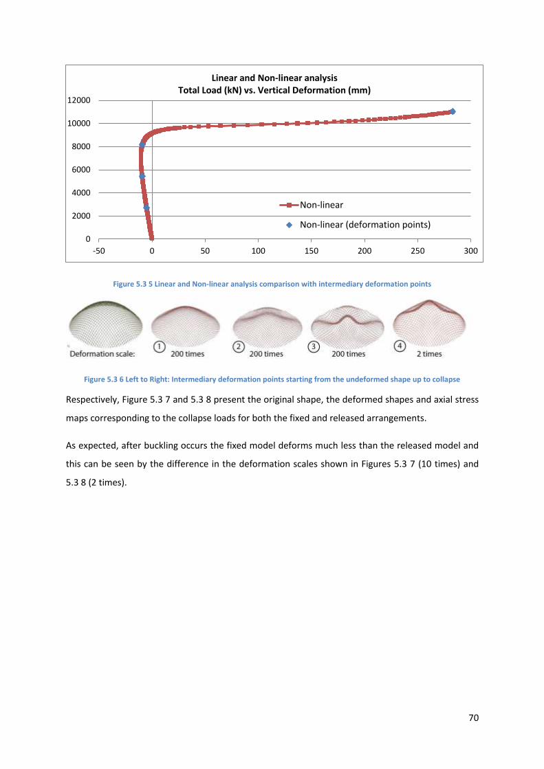
70

Figure 5.3 5 Linear and Non-linear analysis comparison with intermediary deformation points

Figure 5.3 6 Left to Right: Intermediary deformation points starting from the undeformed shape up to collapse

Respectively, Figure 5.3 7 and 5.3 8 present the original shape, the deformed shapes and axial stress

maps corresponding to the collapse loads for both the fixed and released arrangements.

As expected, after buckling occurs the fixed model deforms much less than the released model and

this can be seen by the difference in the deformation scales shown in Figures 5.3 7 (10 times) and

5.3 8 (2 times).

0

2000

4000

6000

8000

10000

12000

-50 0 50 100 150 200 250 300

Linear and Non-linear analysis Total Load (kN) vs. Vertical Deformation (mm)

Non-linear

Non-linear (deformation points)

71

Figu

re 5

.3 7

Do

ub

le-l

aye

red

Off

set-

Fix

ed

. Le

ft:

Un

de

form

ed

sh

ape

. Mid

dle

: D

efo

rme

d s

hap

e R

igh

t: A

xia

l Str

ess

Map

s w

ith

Sca

le

72

Figu

re 5

.3 8

Do

ub

le-l

aye

red

Off

set-

Re

leas

ed

Le

ft:

Un

de

form

ed

sh

ape

. Mid

dle

: D

efo

rme

d s

hap

e R

igh

t: A

xia

l Str

ess

Map

s w

ith

Sca

le

73

5.3.2 Connection Stiffness

Similarly to the single-layered model, the connector setup allowed for modifications in the bending

stiffness of the connectors that would reflect the shear stiffness of the gridshell. Firstly, the size

parameters of the middle connector were modified in the same range as described in Section 5.2.2.

For the very low values, the model describes two single-layered gridshells arranged on top of each

other with a very weak connection in between them. For this analysis, three phase-change loads

have been identified:

1) Start of non-linear behaviour/End of linear behaviour

2) Buckling load

3) Ultimate elastic collapse load.

Figure 5.3 9 shows the effect of the middle connector bending stiffness ( ) on the load carrying

behaviour of double-layered gridshells. is plotted on the horizontal axis using a logarithmic scale

(base 10) while the three loads identified above are plotted along the vertical axis. The same values

are also plotted against the connector sizes used in the different models (Fig 5.3 10).

Figure 5.3 9 Collapse Load, Buckling Load and Non-linear Start Load against connector EI on a logarithmic scale (base 10)

The same behaviour across the range as in the case of the single-layered model is evident here with

very small values of load being achieved at the low end of the range followed by a sharp increase

and capped by a levelling of the values. In this case, the ratio of high to low for the Buckling load is

9.1 : 1 whereas for the Collapse load it is 10.1 : 1. These values are similar to the single layered case

The ratios obtained from this investigation are smaller than the theoretical 13 : 1 value described in

Section 2.1. The reason for this is that the theoretical range covers the domain 0 to whereas our

values only approach 0 and go up to a stiffness corresponding to the 200 x 200 mm connector. In

0

2000

4000

6000

8000

10000

12000

14000

0.01 1 100 10000 1000000 100000000 1E+10 1E+12

Elastic Collapse Load, Buckling Load and Non-linear Start Load (kN) vs EI (Nmm2)

Collapse Load (kN)

Buckling Load (kN)

Non-Linear Start (kN)

74

addition, at the high end of the range, marginal increases still occur, but these are below 0.5% per

order of magnitude of EI.

Figure 5.3 10 Collapse Load, Buckling Load and Non-linear Start Load against connector size (mm)

Furthermore, in order to better understand the deformation behaviour under different stiffness

conditions, the mid-span grid element vertical deformations have been plotted against (Figure 5.3

11) and against the sizes used (Figure 5.3 12).

The two modes of behaviour are more obvious in this case as in the single-layered analysis. The

range can be split approximately in half with the low end featuring increasing downward deflections

of the mid-span. Between the models with 15 x 15 mm and 20 x 20 mm connectors there is a

sudden change in the deformation pattern with the mid-span now deforming upwards. The values

corresponding to the non-linear start load are all negative (showing downward deformation) and

very small (up to 12 mm) in comparison to the other two series shown on the graph.

Figure 5.3 11 Mid-span Vertical Deflections against connector EI corresponding to the loads in Figures 5.3 9 and 5.3 10

0

2000

4000

6000

8000

10000

12000

14000

0.1 0.75 5 10 15 20 30 50 75 100 200

Elastic Collapse Load, Buckling Load and Non-linear Start Load (kN) vs Size (mm)

Collapse Load (kN)

Buckling Load (kN)


-800

-600

-400

-200

0

200

400

0.01 1 100 10000 1000000 100000000 1E+10 1E+12

Vertical Deflection (mm) vs EI (Nmm2)

Buckling Load (kN)


Collapse Load (kN)

75

Figure 5.3 12 Mid-span Vertical Deflections against connector size corresponding to the loads in Figures 5.3 9 and 5.3 10

Finally, given the nature of the double-layered model making use of three sets of connectors, it was

deemed necessary to investigate the effect of modifying all three sets, as opposed to just the middle

one. The following series of graphs (Figures 5.3 13, 5.3 14 and 5.3 15) show the load versus stiffness

comparisons for all three phase-change loads.

Figure 5.3 13 Middle connector modified and All 3 connectors modified Collapse Load against connector EI

Figure 5.3 14 Middle connector modified and All 3 connectors modified Buckling Load against connector EI

-800

-600

-400

-200

0

200

400

0.1 0.75 5 10 15 20 30 50 75 100 200

Vertical Deflection (mm) vs Size (mm)

Collapse Load (kN)

Buckling Load (kN)


0

2000

4000

6000

8000

10000

12000

0.01 1 100 10000 1000000 100000000 1E+10 1E+12

Elastic Collapse Load (kN) vs EI (Nmm2)

Middle connector modified

3 connectors modified

0

2000

4000

6000

8000

10000

12000

0.01 1 100 10000 1000000 100000000 1E+10 1E+12

Buckling Load (kN) vs EI (Nmm2)



76

Figure 5.3 15 Middle connector modified and All 3 connectors modified Non-linear Start Load against connector EI

The behaviour clearly indicates that as all three connectors are now modified in size, the overall

stiffness at each node is significantly reduced for most situations. Therefore, the load values

obtained are smaller than in the cases where only the middle connector was modified. This happens

for the models up to the value of 50 x 50 mm which is identical in both situations, after which the

three connector models show a slightly higher value (2% higher for 200 x 200 mm, collapse load).

This is according to expectations as a consequence of the higher stiffness.

In addition, the vertical deformations of the mid-span grid element were plotted again for this series

of models and are shown following to the same values for the models with middle connector

modifications only (Figures 5.3 16 and 5.3 17).

Figure 5.3 16 Middle connector modified Vertical mid-span deflection across the connector size range

0

2000

4000

6000

8000

10000

12000

0.01 1 100 10000 1000000 100000000 1E+10 1E+12

Non-linear Start Load (kN) vs EI (Nmm2)



-800

-600

-400

-200

0

200

400

0.1 0.75 10 20 30 50 75 100 200

Middle connector modified - Deflection (mm) vs Size (mm)

Collapse Load (kN)

Buckling Load (kN)


77

Figure 5.3 17 All 3 connectors modified Vertical mid-span deflection across the connector size range

As another measure of comparison the load-deformation curves for each series of models were

plotted together and they are show below (Figures 5.3 18, 5.3 19, 5.3 20 and 5.3 21).

Figure 5.3 18 Load-deformation curves for the middle connector modified series

Figure 5.3 19 Load-deformation curves for the middle connector modified series. Range -150 mm to +150 mm

-800

-600

-400

-200

0

200

400

0.1 0.75 10 20 30 50 75 100 200

3 Connectors modified - Deflection (mm) vs Size (mm)

Collapse Load (kN)

Buckling Load (kN)


0

2000

4000

6000

8000

10000

12000

-800 -600 -400 -200 0 200 400

Load-Deformation for the model series with middle connector modified

0.10.755101520305075100200

0

2000

4000

6000

8000

10000

12000

-150 -100 -50 0 50 100 150

Load-Deformation for the model series with middle connector modified

0.1

0.75

5

10

15

20

30

50

75

100

200

78

Figure 5.3 20 Load-deformation curves for the 3 connectors modified series

Figure 5.3 21 Load-deformation curves for the 3 connectors modified series. Range -150 mm to +150 mm

The behaviour of the two series is very similar, the only major difference coming from a shift in the

values where the change in buckling and post-buckling behaviour occurs. As a result of the reduced

overall stiffness per node when all three connectors are modified, the change to upward buckling

now occurs between the values of 20 x 20 mm and 30 x 30 mm.

Noticeably, the curves for the low end of the range studied (0.1 mm up to 10 mm) are much

shallower, confirming the reduced overall stiffness of the nodes and of the entire structure.

Dicussion

The property of the connectors to be rotationally free around their local X-axis results in a lower

capacity of the gridshell while fixing them is, as discussed by Happold and Liddel (1975), one way to

improve the diagonal stiffness of the gridshell and therefore increasing its capacity to carry loads.

0

2000

4000

6000

8000

10000

12000

-800 -600 -400 -200 0 200 400

Load-Deformation for the model series with 3 connectors modified

0.1

0.75

10

20

30

50

75

100

200

0

2000

4000

6000

8000

10000

12000

-150 -100 -50 0 50 100 150

Load-Deformation for the model series with 3 connectors modified

0.1

0.75

10

20

30

50

75

100

200

79

In addition, the relationship between the connector stiffness and buckling load is confirmed to be

consistent with the single-layered model. Furthermore, the ratios between the loads at the high and

low ends of the range are lower than the theoretical 13 : 1 value discussed in Section 2.1 due to the

reasons detailed above.

The values for the highest buckling load of the single-layered model and the buckling load

corresponding to the 0.75 x 0.75 mm middle connector modified double-layered model are in a ratio

of 1 to 2. This proves that a double-layered gridshell with a very weak connection between the two

layers would effectively carry as much load as two independent single-layered gridshells.

Finally, the connector system allows for various modifications to be made to the model investigated

and would be a useful tool in the design of timber gridshells with complex layering systems.

80

5.4 Double Layered Model - Imperfection Analysis The research carried out since the middle of the XX-th century on gridshells has placed a significant

amount of emphasis on the effect of imperfections. Our investigation attempts to look at the

double-layered model by applying two types of imperfections, one related to the stiffness of the

connectors and the other one to geometric conditions (Figure 5.4 1).

Figure 5.4 1 Imperfections. Left: Perfect model. Middle: Local stiffness imperfection. Right: Local geometric imperfection

5.4.1 Connection Stiffness Imperfection

Firstly, a local imperfection at one of the nodes would represent a weakness in one of the

connections of a timber gridshell. In order replicate this, a node location was chosen at a node of no

particular topological significance (i.e. not close to the supports, or mid-span). For this node only, all

three connectors were modified in size and Table 5.1 presents the values used for a series of local

reductions in the connector stiffness ( ).

Connector

Size (mm)

Perfect Model 2% 3% 5% 94%

50 49.75 49.62 49.36 25

( ) 11000 11000 11000 11000 11000

( )

( )

Table 5. 1 Local stiffness imperfection range

The resulting load-deformation curves were plotted together against the baseline perfect model and

this is shown in Figure 5.4 2. For the 2% reduced model, there is no significant difference that

appears in the load carrying behaviour or the capacity of the gridshell. However, for the values of 3%

and 5% there are two different and sudden deviations from the load-deformation curve that occur at

the same value.

81

In order to further investigate this matter, another run was carried out which halved the size of the

connector to 25 x 25 mm leading to an overall decrease in the EI of 94%. The same type of sudden

change occurs around the same value on the load-deformation curve.

As a consequence, it can be said that the model used together with Robot’s analysis may be very

sensitive to imperfections.

Figure 5.4 2 Load-deformation curves for the stiffness imperfections series

The behaviour of the imperfect models presents significant differences between themselves and in

relation to the perfect model.

The following series of figures present the different deformed shapes obtained from the analysis,

together with the associated axial stress maps (Figures 5.4 3, 5.4 4, 5.4 5 and 5.4 6). The undeformed

shapes are also shown with a specific indication on where the imperfection is applied. The same

deformation scale is used for all four pictures (2 times).

0

2000

4000

6000

8000

10000

12000

-150 -100 -50 0 50 100 150 200 250 300

Load-Deformation for the model series with stiffness imperfection

Perfect Model

3% local reduction

2% reduction

5% local reduction

94% local reduction

82

Figu

re 5

.4 3

Sti

ffn

ess

re

du

ctio

n 2

% L

eft

: Un

de

form

ed

sh

ape

. Mid

dle

: D

efo

rme

d s

hap

e. R

igh

t: A

xia

l Str

ess

Map

s w

ith

Sca

le.

Re

d c

ircl

e in

dic

ate

s lo

cati

on

of

the

imp

erf

ect

ion

.

83

Figu

re 5

.4 4

Sti

ffn

ess

re

du

ctio

n 3

% L

eft

: Un

de

form

ed

sh

ape

. Mid

dle

: D

efo

rme

d s

hap

e. R

igh

t: A

xia

l Str

ess

Map

s w

ith

Sca

le.

Re

d c

ircl

e in

dic

ate

s lo

cati

on

of

the

imp

erf

ect

ion

.

84

Figu

re 5

.4 5

Sti

ffn

ess

re

du

ctio

n 5

% L

eft

: Un

de

form

ed

sh

ape

. Mid

dle

: D

efo

rme

d s

hap

e. R

igh

t: A

xia

l Str

ess

Map

s w

ith

Sca

le.

Re

d c

ircl

e in

dic

ate

s lo

cati

on

of

the

imp

erf

ect

ion

.

85

Figu

re 5

.4 6

Sti

ffn

ess

re

du

ctio

n 9

4%

Le

ft: U

nd

efo

rme

d s

hap

e. M

idd

le:

De

form

ed

sh

ape

. Rig

ht:

Axi

al S

tre

ss M

aps

wit

h S

cale

.

Re

d c

ircl

e in

dic

ate

s lo

cati

on

of

the

imp

erf

ect

ion

.

86

Discussion

The deformed shapes are extremely different in comparison to each other and neither is

symmetrical about both axes, as expected. However, they do present symmetry along one direction.

In addition, the 2% limit has been identified as the limit above which the behaviour of the double-

layered model becomes unstable.

These results cannot be interpreted correctly with the amount of data available and further work is

required to establish the exact causes for this. However, there are two major possibilities for the

sudden jumps in the load-deformation curves:

The model itself is extremely sensitive to deviations from the perfect state;

Robot and the analysis method used are extremely sensitive to these deviations and

significantly increasing the number of load increments could be one solution.

5.4.2 Geometrical Imperfection at Node

In order to compare the previous models with the one that looks at geometric imperfections the

same node was chosen as described above. A local geometric imperfection of 5 % was introduced by

modifying the position of the node along one of the lath directions by a margin of 5 % relative to the

distance between the two adjacent nodes (Figure 5.4 1). The results of the load-deformation curve

are presented below alongside the one for the perfect model (Figure 5.4 7).

Figure 5.4 7 Load-deformation comparison between the perfect model and the one with a local geometric imperfection

The same sudden change occurs as in the stiffness imperfection analysis but at a lower value of the

applied load. What’s more, the post-change behaviour is more controlled than in the other

instances, continuing on a gradually increasing slope. Furthermore, the deformed shape can be seen

below together with the undeformed shape and surface location of the imperfection and the axial

stress map (Figure 5.4 8).

0

2000

4000

6000

8000

10000

12000

-50 0 50 100 150 200 250 300

Load-Deformation: Perfect Model vs Geometric Imperfection Model

Perfect Model

5% Local Geometric Imperfection

87

Figu

re 5

.4 8

Ge

om

etr

ic Im

pe

rfe

ctio

n 5

% L

eft

: U

nd

efo

rme

d s

hap

e. M

idd

le:

De

form

ed

sh

ape

. Rig

ht:

Axi

al S

tre

ss M

aps

wit

h S

cale

.

Re

d c

ircl

e in

dic

ate

s lo

cati

on

of

the

imp

erf

ect

ion

wh

ich

is t

he

sam

e a

s fo

r th

e m

od

el w

ith

sti

ffn

ess

imp

erf

ect

ion

88

5.4.3 Asymmetric Loading

One important factor that affects the behaviour of gridshells is the situation where asymmetric

loading occurs. This is most often the case in practice where snow and wind loads occur, possibly

with catastrophic effects as in the case of the Bucharest dome failure.

As such, the double-layered gridshell model was loaded on half of its surface and the same type of

analysis was performed. The load-deformation curve, compared to the symmetric loading on a

perfect model is shown below followed by the deformed shape and axial stresses (Figure 5.4 9).

Figure 5.4 9 Load-deformation comparison between the perfect model and the asymmetrically loaded one

The non-linear behaviour of this model is similar to that of the uniformly distributed applied load

model and doesn’t present any sudden changes. The elastic collapse load is 2.2 times smaller than

that of the perfect model. In addition, as Figure 5.4 10 shows, the deformation keeps its symmetrical

pattern across the one symmetry line of the loaded model (splitting the loaded area in two).

0

2000

4000

6000

8000

10000

12000

-50 0 50 100 150 200 250 300

Load-Deformation: Perfect Model Symmetric vs Asymmetric Loading

Perfect Model

Perfect Model with Asymmetric Loading

89

Figu

re 5

.4 1

0 A

sym

me

tric

Lo

ad o

ver

hal

f o

f th

e a

rea

Left

: Un

de

form

ed

sh

ape

. Mid

dle

: D

efo

rme

d s

hap

e. R

igh

t: A

xial

Str

ess

Map

s w

ith

Sca

le.

Re

d a

rro

ws

ind

icat

e w

he

re t

he

load

is.

90

5.5 Critique on Robot Structural Analysis Robot is an extremely capable structural analysis and design package and it offers a variety of

options in terms of handling the non-linear analysis performed on the models discussed in this

thesis.

The calculation time required for the typical models investigated, involving a number of increments

of 300 to 400, is shown below in Table 5.5 1 together with the corresponding number of equations

that needed to be solved.

Single Layered Model Double Layered Model

Number of equations 12,912 26,064

Calculation time13 Between 45 and 115 minutes Between 120 and 180 minutes

Table 5.5 1 Calculation times for both types of models using Robot

These are sufficiently reasonable working parameters but for more complex structures with

increasing numbers of elements, higher processing power may be required or a simplification of the

model, either by making use of lines of symmetry or by reducing the complexity.

Furthermore, one significant drawback of Robot was its inability to present real-time results as the

load increments increase or to pause at intermediary steps in order to be able to visualise and save

deformation or stress patterns.

One of the most negative aspects which encumbered this investigation was Robot’s sensitivity to the

values of the load increments. For example, some analysis runs obtained asymmetrical deformations

for perfectly symmetrical models. Changing the tolerances and convergence parameters made no

effect and the only solution was to apply a different load that would then be split into increments at

different values which ultimately lead to a symmetrical solution.

13

On a Windows 7 machine with Intel Core i3 CPU @3.07GHz and 4.00GB RAM

91

5.6 Applicability of these Results towards Design The results presented in this thesis can be used for future timber gridshell designs in two different

contexts and are applicable in both the scheme and detailed design phase.

Firstly, by making use of dimensional analysis, it is possible to scale the results in order to evaluate

the performance of a structure that is similar to the prototype investigated, but which has different

dimensions. Simply put, if the whole geometry is scaled, including member sizes, the capacity per m2

would be the same as in this case, with the provision that the self-weight would also carry a scaled

proportion of this capacity. Happold and Liddell (1975) explain how this can be achieved from scale

models to predict full-size building behaviour and the method is based on the detailed description of

dimensional analysis provided by Buckingham (1914).

Secondly, the results presented here can be used to calibrate the computer analysis during the

design process. Information about how to replicate the models investigated here is available in

Section 3 with regard to the geometric definition and in Section 4 with regard to the structural

modelling, material properties and analysis method.

92

6. Conclusion

This thesis presented an in-depth review of timber gridshell construction technology, within a wide

architectural and engineering framework concerned with the design and construction of the projects

that have been built so far. The specificities of timber as a construction material for gridshells have

been outlined and compared to steel, while the use of timber in construction has been placed in the

current context of environmental awareness.

Through the study of precedents, it has become evident that timber gridshells are a very effective

means to cover large areas and span long distances. Structurally, they act in a similar manner as

continuous shells, but there are significant differences as well. By concentrating the material of a

shell into long strips, the paths of direct forces are now directionally limited and there is therefore a

need to introduce some form of diagonal resistance.

In contrast with discrete member steel gridshells, which have multiple members connecting at the

same node, continuous member timber gridshells feature sets of laths which are stacked onto each

other creating a layering system that eliminates the need for complicated geometry connections at

the nodes, thus allowing for standardisation.

In addition, timber gridshells have proven to be an extremely cost effective way to cover large areas,

while the use of timber as primary construction material, adequately sourced, is beneficial for the

environment.

Most importantly, through the limited number of projects realised so far it has been clear that the

potential for innovation, both in structural design and in architectural expression, is vast and that

the last decade has seen the timber gridshell technology closer to entering the mainstream of UK

lightweight construction.

Furthermore, the experimental nature of the design process has become evident and this is

adequate for an innovative type of structure. However, as timber gridshells become more popular, it

is necessary to have a certain amount of independence from this in order to reduce cost and

increase confidence. As a consequence, this work puts forward a proposal for a structural model that

would be able to accurately simulate the unique layering system of timber gridshells. The model was

then used in a numerical non-linear elastic analysis programme that investigated the behaviour of

timber gridshells. This thesis looked at both single-layered and double-layered timber gridshell

models.

93

Firstly, a simple computational prototype was developed within a parametric framework that

allowed for the definition of the geometry and which was the basis for the structural model.

Secondly, using Autodesk Robot Structural Analysis, more than 50 variations of this model were

investigated. In order to build confidence in the non-linear method used, a simple 2D arch model

was analysed and the results were compared to two independent analyses. It was found that the

non-linear method used by Robot provided accurate results and it was deemed appropriate for use

in the timber gridshell model.

The fundamental characteristic of the structural model proposed is the introduction of short

connector elements between the different layers of the gridshell. These introduce an offset that

accurately represents the layering system encountered in timber gridshells and this allows us to

examine the relationship between the behaviour of the gridshell and two distinct properties:

the torsional resistance of the connectors, which can be used to simulate rotational freedom

at the nodes, and

the bending stiffness of the connectors, which can be used as a representation of the shear

stiffness of the gridshell itself.

By applying this to a single-layered model (one set of laths in each direction) it was found that when

the connectors have zero torsional rigidity (achieved by using releases in Robot) the buckling load

was 47% of that of a model with fully fixed connectors. The same setup was used for a double-

layered model (two sets of laths in each direction), which featured three connectors per node, and

the released model buckling load was found to be 83% of the fully fixed value.

Furthermore, connector size variations were used to achieve a range of stiffness and both the single-

layered and the double-layered models were subject to a set of analyses. It was found that both

presented a similar variation of their capacity across the stiffness range:

at the lower end the capacity of the gridshells was very limited;

the middle part of the range showed a gradual and steady increase;

at the higher end (around the size equivalent representative of a real structure) the capacity

begins to stabilise, regardless of any further increases in the connector stiffness.

The deformation behaviour was also an extremely important part of this investigation and the

models exhibited small deformations for pre-buckling states, consistent with the behaviour of shells

acting under direct compression, and large displacements after buckling. It was also noted that

buckling was spread over areas of the gridshell.

94

Finally, as material and geometric imperfections constitute a topic of interest in the study of

gridshells, the double-layered model was altered and the effect of local stiffness and of local

geometric imperfections at a node was examined. The results showed that either the model or the

analysis method is very sensitive towards imperfect structures, yielding significant changes in the

load-deformation behaviour and a reduction in the overall capacity. There is a need for future work

in this area, with a specific focus on issues that affect the translation of a timber gridshell design into

reality.

Future Work As a confirmation of the suitability of the connector model proposed in this thesis, it would be useful

to have experimental results that would help assign accurate information about the nodal

connection behaviour to the connectors (including shear, friction and torsion).

Furthermore, as mentioned above, more work is needed to explore the exact degree of sensitivity

towards imperfections of this model.

From a computational process point of view, it is possible to reduce the complexity of double-

layered or maybe even triple-layered gridshell models by using a smaller number of layers with

effective properties corresponding to the desired arrangement. However, as computational

capabilities constantly increase, such a reduction would no longer bring any work-time benefits.

Finally, the most fertile ground for timber gridshell research is the possibility of parametrically

exploring variable gridshell thickness and surface pattern options that could be adjusted in a design

loop (geometry – analysis – new geometry). The connector model proposed here would be very

useful in changing the thickness locally, helping create an optimised gridshell for specific geometric

and loading conditions.

95

References

Architect's Journal, Building Library. Availaibe: http://www.ajbuildingslibrary.co.uk/ [Accessed 12

October 2012]

Architects, S.P., Scunthorpe Sports Academy [Online]. Available: http://www.s-parchitects.com/

[Accessed 4 October 2012].

Autodesk, 2012. Robot Structural Analysis Professional - User's Guide [Online]. Available:

http://docs.autodesk.com/RSA/2012/ENU/landing.html [Accessed 28 August 2012].

Azagra, D. & Hay, T., 2012. A case for physical models. Structural Engineer, 90, 14-20.

Bechthold, M., 2008. Innovative surface structures : technology and applications. London: Taylor &

Francis.

Brown, S., 2005. Millennium and beyond. Structural Engineer, 83, 34-42.

Buckingham, E., 1914. On Physically Similar Systems; Illustrations of the Use of Dimensional

Equations. Physical Review, 4, 345-376.

Bulenda, T. & Knippers, J., 2001. Stability of grid shells. Computers and Structures, 79, 1161-1174.

Calladine, C.R., 1983. Theory of shell structures. Cambridge: Cambridge : Cambridge University Press.

Douthe, C., Baverel, O. & Caron, J.F., 2006. Form-finding of a grid shell in composite materials.

Journal of the International Association for Shell and Spatial Structures, 47, 53-62.

Gambhir, M.L., 2004. Stability analysis and design of structures. Berlin ; New York: Springer.

Gioncu, V., 1995. Buckling of reticulated shells. State-of-the-art. International Journal of Space

Structures, 10, 1-1.

Gridshell.it, 2012. Form resistant lightweight timber structures [Online]. Available:

http://www.gridshell.it/category/structures/ [Accessed 30 August 2012].

Happold, E. & Liddell, W.I., 1975. Timber Lattice Roof for the Mannheim Bundesgartenschau.

Structural Engineer, 53, 99-135.

Happold, E. & Liddell, W.I., 1976. Discussion - Timber Lattice Roof for the Mannheim

Bundesgartenschau. Structural Engineer, 54, 247-257.

Harris, R., 2004. 21st century timber engineering - The age of enlightenment for timber design Part

1: An introduction to timber. Structural Engineer, 82, 52-57.

Harris, R., Year. 21st century timber engineering - The age of enlightenment for timber design Part 2:

Environmental credentials. In, 2005. Institution of Structural Engineers, 23-28.

Harris, R., 2006. Savill Building: A new landmark for Windsor Great Park. Structural Engineer, 84, 16-

19.

Harris, R., 2011. Design of timber gridded shell structures. Proceedings of the Institution of Civil

Engineers: Structures and Buildings, 164, 105-116.

http://www.ajbuildingslibrary.co.uk/

http://www.s-parchitects.com/

http://docs.autodesk.com/RSA/2012/ENU/landing.html

http://www.gridshell.it/category/structures/

96

Harris, R., Dickson, M., Kelly, O. & Roynon, J., 2004. The Use of Timber Gridshells for Long Span

Structures. 8th International Conference on Timber Engineering. Lahti, Finland: WCTE.

Harris, R., Haskins, S. & Roynon, J., 2008. The Savill Garden gridshell: Design and construction.


Harris, R., Kelly, O. & Dickson, M., 2003a. Downland gridshell - An innovation in timber design.

Proceedings of the Institution of Civil Engineers: Civil Engineering, 156, 26-33.

Harris, R., Romer, J., Kelly, O. & Johnson, S., 2003b. Design and construction of the Downland

Gridshell. Building Research and Information, 31, 427-454.

herzogenriedpark.de, 2012. Architektonischer Vorreiter unter Denkmalschutz [Online]. Available:

http://www.herzogenriedpark.de/mein-herzogenriedpark/multihalle [Accessed 22 August 2012].

Jensen, 2001. The Downland grid shell. Structural Engineer, 79, 16-16.

Jombert, C.-A., 1779. Elevation de la face du Pantheon, a Rome.

Kelly, O.J., Harris, R.J.L., Dickson, M.G.T. & Rowe, J.A., 2001. Construction of the downland gridshell.


Koiter, W.T., 1967. On the stability of elastic equilibrium. Washington,: National Aeronautics and

Space Administration,.

Lewis, B., 2011. Centre Pompidou - Metz: Engineering the roof. Structural Engineer, 89, 20-25.

Malek, S.R., 2012. The Effect of Geometry and Topology on the Mechanics of Grid Shells. Doctor of

Philosophy, Massachusetts Institute of Technology.

Merrick, J., 2006. This is not bling, nor even duchy original - Building Study. The Architect's Journal.

multihalle.de, 2012. Restaurant Multihalle [Online]. Available: http://multihalle.de/ [Accessed 22

August 2012].

Natterer, J., Burger, N., ller, A. & Natterer, J., 2000. Roof of the Main Hall at EXPO 2000 in Hanover,

Germany. Structural Engineering International, 10, 167-169.

Natterer, J. & MacIntyre, J., 1993. Polydome: A Timber Shell, Switzerland. Structural Engineering

International, 3, 82-83.

Natterer, J. & Weinand, Y., Year. Modelling of multi layer beam with inter-layer slips. In: 10th World

Conference on Timber Engineering 2008, June 2, 2008 - June 5, 2008, 2008 Miyazaki, Japan.

Engineered Wood Products Association, 2181-2188.

Officer, L.H. & Williamson, S.H., http://www.measuringworth.com/ [Online]. Available:

http://www.measuringworth.com/ [Accessed 23 July 2012].

Olcayto, R., 2007. Gridshell glazes over the past [Online]. Building Design Online. Available:

http://www.bdonline.co.uk/buildings/technical/gridshell-glazes-over-the-

past/3089698.article [Accessed 30 August 2012].

http://www.herzogenriedpark.de/mein-herzogenriedpark/multihalle

http://multihalle.de/

http://www.measuringworth.com/

http://www.measuringworth.com/

http://www.bdonline.co.uk/buildings/technical/gridshell-glazes-over-the-past/3089698.article

http://www.bdonline.co.uk/buildings/technical/gridshell-glazes-over-the-past/3089698.article

97

Parliament, 2008. Climate Change Act. In: Parliament, (ed.).

Pearman, H., 2000. Empire in the sun. The Sunday Times. London.

Pearman, H., 2002. Blending into the woodland, creaking gently in the breeze, the Gridshell is the

perfect rural building. The Sunday Times. London.

Pearman, H., 2006. Grounds for optimisim. The Sunday Times. London.

sbp, Courtyard of the Palacio de Comunicaciones [Online]. Available:

http://www.sbp.de/en#build/show/1422-Palacio_de_Comunicaciones_courtyard_roof

[Accessed 15 October 2012].

SMDArquitectes, Case Study: Mannheim Multihalle [Online]. Available:

http://www.smdarq.net/case-study-mannheim-multihalle/ [Accessed 5 October 2012].

Sociedad, L.D., 2010. Gallardón corona su "pirámide" con una bóveda de cristal de 5 millones de

euros [Online]. Available: http://www.libertaddigital.com/sociedad/gallardon-corona-su-

piramide-con-una-boveda-de-cristal-de-5-millones-de-euros-1276395429/ [Accessed 15

October 2012].

Timoshenko, S.P. & Timoshenko, S.P., 1953. History of strength of materials. London: McGraw-Hill

Book Company.

TRADA, 2007. The Savill Building, Windsor Great Park [Online]. Available:

http://www.trada.co.uk/casestudies/overview/SavillBuilding/ [Accessed 30 August 2012].

TRADA, 2012. Western hemlock [Online]. Timber Species Database. Available:

http://www.trada.co.uk/techinfo/tsg/view/33 [Accessed 22 August 2012].

Weinand, Y. & Pirazzi, C., 2006. Geodesic Lines on Free-Form Surfaces - Optimized Grids for Timber

Rib Shells. World Conference in Timber Engineering WCTE. Portland, USA.

Williams, C.J.K., 2001. The analytic and numerical definition of the geometry of the British Museum

Great Court Roof. Mathematics & Design. Geelong, Australia: Deakin University.

Worrell, E., Price, L., Martin, N., Hendriks, C. & Meida, L.O., 2001. Carbon dioxide emissions from the

global cement industry. Annual Review of Energy and the Environment, 26, 303-329.

Wright, D.T., 1965. Membrane forces and buckling in reticulated shells. American Society of Civil

Engineers Proceedings, Journal of the Structural Division, 91, 173-201.

Yamashita, T. & Kato, S., 2001. Elastic buckling characteristics of two-way grid shells of single layer

and its application in design to evaluate the non-linear behavior and ultimate strength.

Journal of Constructional Steel Research, 57, 1289-1308.

Zingoni, A., 1997. Shell structures in civil and mechanical engineering : theory and closed-form

analytical solutions. London: London : Thomas Telford.

http://www.sbp.de/en#build/show/1422-Palacio_de_Comunicaciones_courtyard_roof

http://www.smdarq.net/case-study-mannheim-multihalle/

http://www.libertaddigital.com/sociedad/gallardon-corona-su-piramide-con-una-boveda-de-cristal-de-5-millones-de-euros-1276395429/

http://www.libertaddigital.com/sociedad/gallardon-corona-su-piramide-con-una-boveda-de-cristal-de-5-millones-de-euros-1276395429/

http://www.trada.co.uk/casestudies/overview/SavillBuilding/

http://www.trada.co.uk/techinfo/tsg/view/33

geometry and performance of timber gridshells naicu, dragos

Documents