geometry and mechanics of pneumatic tireswanderlodgegurus.com/database/theory/tiregeometry.pdf ·...
TRANSCRIPT
GEOMETRY AND
MECHANICS OF
PNEUMATIC TIRES
F. KOUTNÝ
_______________________________
Zlín, CZE • 2007
- -
F. KOUTNY: GEOMETRY AND MECHANICS OF PNEUMATIC TIRES
I
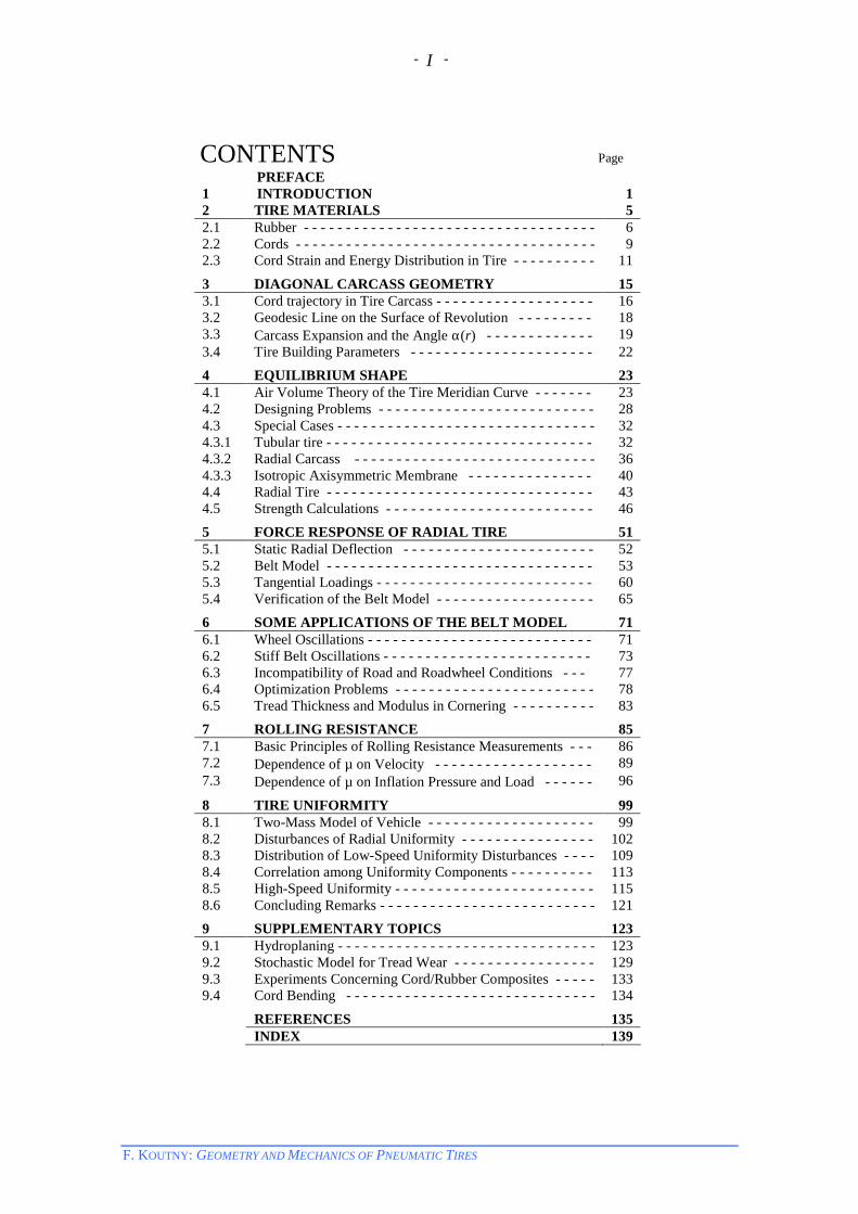
CONTENTS Page PREFACE 1 INTRODUCTION 1 2 TIRE MATERIALS 5 2.1 Rubber - - - - - - - - - - - - - - - - - - - - - - - - - - - - - - - - - - - 6 2.2 Cords - - - - - - - - - - - - - - - - - - - - - - - - - - - - - - - - - - - - 9 2.3 Cord Strain and Energy Distribution in Tire - - - - - - - - - - 11
3 DIAGONAL CARCASS GEOMETRY 15 3.1 Cord trajectory in Tire Carcass - - - - - - - - - - - - - - - - - - - 16 3.2 Geodesic Line on the Surface of Revolution - - - - - - - - - 18 3.3 Carcass Expansion and the Angle α(r) - - - - - - - - - - - - - 19 3.4 Tire Building Parameters - - - - - - - - - - - - - - - - - - - - - - 22
4 EQUILIBRIUM SHAPE 23 4.1 Air Volume Theory of the Tire Meridian Curve - - - - - - - 23 4.2 Designing Problems - - - - - - - - - - - - - - - - - - - - - - - - - - 28 4.3 Special Cases - - - - - - - - - - - - - - - - - - - - - - - - - - - - - - - 32 4.3.1 Tubular tire - - - - - - - - - - - - - - - - - - - - - - - - - - - - - - - - 32 4.3.2 Radial Carcass - - - - - - - - - - - - - - - - - - - - - - - - - - - - - 36 4.3.3 Isotropic Axisymmetric Membrane - - - - - - - - - - - - - - - 40 4.4 Radial Tire - - - - - - - - - - - - - - - - - - - - - - - - - - - - - - - - 43 4.5 Strength Calculations - - - - - - - - - - - - - - - - - - - - - - - - - 46
5 FORCE RESPONSE OF RADIAL TIRE 51 5.1 Static Radial Deflection - - - - - - - - - - - - - - - - - - - - - - - 52 5.2 Belt Model - - - - - - - - - - - - - - - - - - - - - - - - - - - - - - - - 53 5.3 Tangential Loadings - - - - - - - - - - - - - - - - - - - - - - - - - - 60 5.4 Verification of the Belt Model - - - - - - - - - - - - - - - - - - - 65
6 SOME APPLICATIONS OF THE BELT MODEL 71 6.1 Wheel Oscillations - - - - - - - - - - - - - - - - - - - - - - - - - - - 71 6.2 Stiff Belt Oscillations - - - - - - - - - - - - - - - - - - - - - - - - - 73 6.3 Incompatibility of Road and Roadwheel Conditions - - - 77 6.4 Optimization Problems - - - - - - - - - - - - - - - - - - - - - - - - 78 6.5 Tread Thickness and Modulus in Cornering - - - - - - - - - - 83
7 ROLLING RESISTANCE 85 7.1 Basic Principles of Rolling Resistance Measurements - - - 86 7.2 Dependence of µ on Velocity - - - - - - - - - - - - - - - - - - - 89 7.3 Dependence of µ on Inflation Pressure and Load - - - - - - 96
8 TIRE UNIFORMITY 99 8.1 Two-Mass Model of Vehicle - - - - - - - - - - - - - - - - - - - - 99 8.2 Disturbances of Radial Uniformity - - - - - - - - - - - - - - - - 102 8.3 Distribution of Low-Speed Uniformity Disturbances - - - - 109 8.4 Correlation among Uniformity Components - - - - - - - - - - 113 8.5 High-Speed Uniformity - - - - - - - - - - - - - - - - - - - - - - - - 115 8.6 Concluding Remarks - - - - - - - - - - - - - - - - - - - - - - - - - - 121
9 SUPPLEMENTARY TOPICS 123 9.1 Hydroplaning - - - - - - - - - - - - - - - - - - - - - - - - - - - - - - - 123 9.2 Stochastic Model for Tread Wear - - - - - - - - - - - - - - - - - 129 9.3 Experiments Concerning Cord/Rubber Composites - - - - - 133 9.4 Cord Bending - - - - - - - - - - - - - - - - - - - - - - - - - - - - - - 134
REFERENCES 135 INDEX 139
- -
F. KOUTNY: GEOMETRY AND MECHANICS OF PNEUMATIC TIRES
II
PREFACE This text is based on a compiling work written under the same title in 1996. Thus, it might look a bit old fashioned. But as I am still regularly reading two journals on tires, namely Tire Science and Technology and Tire Technology International, I see that old motives preserve their repeated appearing practically unchanged. That is why I decided to translate the work and update it in view of the present stage of my knowledge. Fast development of electronics, computers, numerical methods and all the complex structure of contemporary science has produced immense packets of specialized knowledge in every technical branch. The mathematical point of view, very often underestimated in the past, has finally found its place also in many areas traditionally considered for purely empirical ones. Tire production and exploitation is one of them. Today mathematical modeling is taken as a necessary part of inventing and designing every new rubber product and a tool to enhancing the quality and efficiency of production processes, accelerating development cycles, removing expensive tests on prototypes etc. The following chapters offer a short look at the tire structure and illustrate nonlinearities in behavior of basic tire materials. The role of the compressed air filling is emphasized by evaluating its prevailing contribution to total energy accumulated in tire. Then the problem of loading the tire structure with the internal air pressure is solved under the assumption that the energy accumulated in tire wall is neglected. This assumption enables setting up the so called belt model and solving simple cases of tire loading in analytical form within a very short time, i.e. instantly from the practical point of view. The belt model may serve in many application areas like rolling resistance, tire uniformity etc. The text may seem to be sometimes too concise. But all the needed mathematics with sufficient details could be found in Courses on this website (www.koutny-math.com). I take it as a shapeable material and may be some supplementary sections could be added in the future. There are also more comprehensive works at hand today like
Mechanics of Pneumatic Tires edited by S. K. Clark or The Pneumatic Tires edited by A. N. Gent and J. D. Walter.
It is just and fair to remind also Russian authors (Biderman, Bukhin and many others) who significantly contributed to the theory of pneumatic tires as well. I would like to apologize for my imperfectness, numerous mistakes, bad formulations and many linguistic trespasses.
F. Koutny
- -
1 INTRODUCTION
F. KOUTNY: GEOMETRY AND MECHANICS OF PNEUMATIC TIRES
1
The mathematician is characterized not by computing but by his clear thinking and his ability to omit irrelevant things.
Rósza Péter
1 INTRODUCTION Various vehicles such as cars and trucks in the first place, tractors, agricultural and forestry machinery etc. as well as aircrafts and jets belong to inevitable technical means of the present time. It is clear that the wheels of high performance vehicles cannot be built somehow by blind trials but modern construction means are needed in their design and development. Computers and robots are attributes of technological development almost in all branches of human activities in the last decade. Outputs of projecting works are completely automated and transferred to CNC machines. Laser optics and CCD cameras are used in optical control, computer tomography creates spatial view of the internal structure of goods etc. So mathematical methods have found a fertile soil also in many areas where they were completely ignored a few years ago. Though the pneumatic tire was invented and patented already in 1845 (Thomson) and reinvented in 1888 (Dunlop) [1] the first theoretical works concerning its construction appeared only in 1950ies (Hofferberth) [2]. The theory, however, was too complicated (integration of a function with a singularity) and its practical applications were conditioned by use of computers that were then only in napkins. In decades 1970 and 1980 graphical-numerical methods were used also and to make their application easier special nomographs were published [3-7]. At that time also analog computers were used to obtain the meridian curve of the tire. But with mass applications of digital computers, especially PC’s, those methods declined very quickly. Developments of electronics and numerical methods have had a strong influence also in various branches of rubber industry (machinery, automating technology, construction, testing). Here the basic knowledge concerning the construction and properties of tires will be discussed. It is obvious that the pneumatic tire as a real object must be represented in a very simplified way if the corresponding mathematical models are to be successful in search for answers to properly formulated questions. Theoretical results of any model need to be compared with the experimental ones whenever possible. As a rule, sooner or later experimental facts are discovered that do not agree with the theoretical predictions. Then the model must be adapted, if possible, or abandoned completely and substituted by a better model. This process is repeated again and again and the spiral-like development is a characteristic feature of general recognition (see Prelude to Probability … on this website).

- -
1 INTRODUCTION
F. KOUTNY: GEOMETRY AND MECHANICS OF PNEUMATIC TIRES
2
Experiment is a basic element of natural and technical sciences. Its reproducibility and repeatability assures the objectivity of science. This feature of experimental work is closely connected to applications of statistical methods.
But let us turn to the object of pneumatic tire again. Radial tire lettering is a sequence of figures and letters with the following meaning:
Outer width (mm) / aspect ratio + (Speed category) R + Rim diameter (inch) + Tread pattern.
Tire wall consists of three main components (Figure 1.1): • approximately homogeneous and isotropic outer rubber layers of the sidewall
and tread with patterned grooves needed for transmission of forces and moments in the interface tire/road,
• reinforced parts (carcass, belt, beads) of cord/rubber composites carrying main part of stresses produced by the internal air overpressure and external dynamic loads between rim and road,
• homogeneous layer of innerliner rubber material with small diffusion coefficient to preserve the inner overpressure in the tire cavity.
This complicated structure is very uncomfortable to describe mathematically. Moreover, there are very large differences in physical characteristics of individual tire layers, significant dependence of rubber behavior (and also of some cords behavior) on temperature, general nonlinearity in stress/strain relation and hysteresis. Also strains that cannot be considered small and tire geometry, though approximated by an axisymmetric body as usual, do not belong to simplifying facts.
Figure 1.1 – A schematic picture of the cross-section of a radial tire.
- -
1 INTRODUCTION
F. KOUTNY: GEOMETRY AND MECHANICS OF PNEUMATIC TIRES
3
The equilibrium shape theory, strength and tire building calculations take into account the load/deflection curves of corresponding reinforcing cords, wires etc. Rubber is considered just as a sealing and completely deformable material. But in calculations of tire reactions to the external loads the deflection of tread must be considered too. Therefore, also basic stress-strain behavior of rubber needs to be somehow described. Traffic safety requires that the tire as a pressure vessel retains its integrity during its whole service life. But its components are exposed to cyclic loadings so their strength drops necessarily. Study of the fatigue behavior of individual tire components in exploitation is expensive, because strengths measurement means total destruction of the tire. E.g. acquiring the bead strength drop after traveling a fixed distance would need a burst test of tire with pressurized water. Preserving the material strength above a given level needs to know something on how it depends on stress-strain conditions and what the working conditions of tire are like. A qualified estimate of deflection of the traveling tire is the first step to it. Conditions in regular exploitation, however, are a mixture of deterministic and stochastic components. Therefore, realistic simulation of the cord loading is very difficult in laboratory. The carcass cord in running tire is periodically unloaded and bent during its passing the contact area. So estimates of the upper and lower levels of the cord tension and deflection would be very useful to describe the fatigue regime. This, however, needs a suitable tire model. Systemizing experimental data can help to reveal some relations (or structures) that in some cases may be explicitly expressed in mathematical form. Mathematical models enable prediction and theoretical results can be confronted with experimental data in the experimentally feasible domains. On the other hand, theoretical results can transcend the possibilities of experiments. A system of ideas, hypothesis or theory can be considered scientific in the sense of K. Popper only if it includes the possibility of its falsifiability, e.g. by experimental disprovability. As far as the horizon of the investigation is broad enough while the area of knowledge is small several concurrent theories may exist contemporarily. The subjective standpoint may be influenced by the temporary philosophy, ideological fashion, social or political boosts or constrictions etc.
The Greek word “pneuma” means the air, which emphasizes etymologically the role of the compressed air in the pneumatic tire. The German “Luftreifen” is the verbatim equivalent of the pneumatic tire. The behavior of the system (tire wall/air) is controlled by the principle of minimum energy. The today so popular finite element method (FEM) finds this minimum via numerical solution of large systems of equations corresponding to individual elements and their constrictions. Neglecting the tire wall energy, however, simplifies the problem
- -
1 INTRODUCTION
F. KOUTNY: GEOMETRY AND MECHANICS OF PNEUMATIC TIRES
4
substantially. This can lead to a relatively simple and analytically solvable problem, whose solution can be obtained very fast by numerical methods. Direct measuring the inflation pressure increase in two car tires during their radial loading in laboratory by mercury manometer [12] provided a justification for such a neglecting. Rhyne’s regression formula for radial stiffness [13] transformed for SI units,
Kz = 1.3368.2 +WDp (p is the inflation pressure in MPa, W and D are the width and diameter of tire in mm), was verified in several large tire groups and confirms the overwhelming role of the compressed air in the pneumatic tire. It gives the ratio of the radial stiffness (N/mm) of a flat tire (p = 0) and the radial stiffness of the same inflated tire
1.3368.21.33
+WDp
As mentioned above, those ideas create a basis of the belt model of radial tire that enables to predict its external behavior, i.e. load/deflection curves in radial, lateral, circumferential directions quite good. It can also be used to predict average stresses in supporting elements inside the tire structure. Nevertheless, computing local stress peaks or determining stresses and strains maps need finer means (FEA). In the tread/road interface local strains are influenced by the macroscopic and microscopic bumps and asperities on the road surface. Corresponding stresses may exceed the critical level of material strength. Then microscopic particles are torn out of the surface. This destructive process is manifested as the tread wear. Wear rate depends on tread rubber compound, road surface quality, interface temperature etc. As said in Preface this text is a commented summary on author’s former publications in different journals. Its main goal is to show that relatively simple methods and means can still be useful in such a large application area like the geometry, technology and mechanics of pneumatic tires.
P

- -
2 TIRE MATERIALS
F. KOUTNY: GEOMETRY AND MECHANICS OF PNEUMATIC TIRES
5
2 TIRE MATERIALS Properties of macromolecular materials for tire production belong in the area of physics of polymers [14]. However, there is a substantial difference in response of real tire compounds and the ideal elastomer considered in the kinetic theory of rubber elasticity. For example, the ideal material is stiffening with increasing temperature while the real tire rubber compounds become softer. To illustrate the complexity of real tire materials several examples are presented below. 2.1 Rubber
Figure 2.1 – Hysteresis loops of the vulcanization bladder rubber in the first and fifth strain cycle.
150°C
70°C
23°C
0
20
1.6 1.4 1.2 1.0
Force, N
10
30
Elongation ratio λ
Force, N
150°C
23°C
70°C
1.6 1.4 1.2 1.0 0
20
10
30
Cycle 1
Cycle 5
Elongation ratio λ
- -
2 TIRE MATERIALS
F. KOUTNY: GEOMETRY AND MECHANICS OF PNEUMATIC TIRES
6
Figure 2.1 demonstrates complexity of stress strain behavior in rubber. There are shown hysteretic loops of test pieces prepared of bladder rubber at different temperatures in the first and the fifth strain cycles. It is surely difficult to clarify what could be meant under the Young modulus in such a case and why. The information value of the Young modulus is low for the majority of the people who develop rubber compounds. On the other hand the evaluation criterions used by those people cannot be used in the regular physical description of rubber. To compute tangential forces in radial tire the shear modulus of tread compound is needed. This, however, is not measured as a rule. To determine the shear stiffness of rubber, the device shown in Figure 2.2 was made. It enabled to record the tensile force F(x) at displacement x of jaws by INSTRON TTCM machine [15]. Though the torque F(x).R represents an average of shear stresses the linear elasticity gives proportionality between the shear modulus G and the ratio F(x)/x. However, tensile force F(x) showed nonlinearity, which implies variability of G with x and the shear angle (Figure 2.3). Both the dynamic (oscillation) and static torsion tests with standard shear test pieces were carried out.
Figure 2.2 – A device for rubber torsion testing either statically on INSTRON TTCM (the distance between horizontal axis and vertical tension axis is the pulley radius) or dynamically by flywheel.

- -
2 TIRE MATERIALS
F. KOUTNY: GEOMETRY AND MECHANICS OF PNEUMATIC TIRES
7
Figure 2.3 – Nonlinear relationship between the displacement of INSTRON jaws and force.
In some parts of the tire the pressure stress is dominant, e.g. in tread. Therefore, also pressure tests were performed on cylindrical test pieces cut out either of laboratory rubber plates [16] or directly from treads of tires [17]. Stress/strain characteristics were taken in the 3rd or 5th strain cycle. To illustrate the dependence on temperature (°C) pressure moduli are shown at different temperatures. In tread compounds an exponential drop with the absolute temperature was ascertained (Figure 2.4). But these approximations cannot be used for extrapolations (e.g. at temperatures lower than 10°C the materials become stiffer than predicted).
4
5
6
7
8
10 30 50 70 90 110Temperature T , °C
Youn
g's
mod
ulus
E, M
Pa E =1.45 exp(476/(273+T ))
E =1.25 exp(478/(273+T ))
Figure 2.4 – Young’s pressure modulus decrease in truck tire treads with increasing temperature; Michelin, ∆ Semperit.
In hysteresis a similar decrease may be observed. Figure 2.5 shows the drop of hysteresis with increasing temperature in rubber matrix of belt cord layer. Hysteresis
- -
2 TIRE MATERIALS
F. KOUTNY: GEOMETRY AND MECHANICS OF PNEUMATIC TIRES
8
losses were calculated directly from force/displacement records of INSTRON 6025. But the resilience measurement by Lüpke method proved to be easier and more acceptable due to lower variance.
30
40
50
60
0 50 100 150Temperature T , °C
100
- Ela
stic
ity L
üpke
, H, %
H =10.79 exp(488.6/(273+T ))
Figure 2.5 – Hysteresis decrease with increasing temperature in belt rubber matrix of a truck tire.
The displayed regression function would reach the level of H = 100% at T ≈ –53°C, i.e. approximately at the glass transition temperature of the rubber. With this temperature the regression functions from Figure 2.4 would be transferred to
EMichelin(T) = 3.85 exp T+53
55.49 , ESemperit(T) = 3.22 exp T+53
95.52 .
Those formulas also adequately fit the experimental data and are acceptable in a broader range of temperature.
0
0.5
1
1.5
2
2.5
1 1.2 1.4 1.6 1.8 2Elongation ratio λ
Stre
ss σ
, N/m
m
Figure 2.6 – Hysteresis loops of rubberized steel cord strip of 50mm width before tire building.
- -
2 TIRE MATERIALS
F. KOUTNY: GEOMETRY AND MECHANICS OF PNEUMATIC TIRES
9
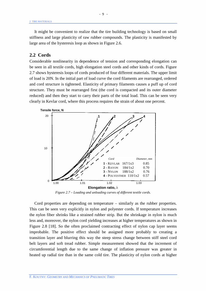
It might be convenient to realize that the tire building technology is based on small stiffness and large plasticity of raw rubber compounds. The plasticity is manifested by large area of the hysteresis loop as shown in Figure 2.6. 2.2 Cords Considerable nonlinearity in dependence of tension and corresponding elongation can be seen in all textile cords, high elongation steel cords and other kinds of cords. Figure 2.7 shows hysteresis loops of cords produced of four different materials. The upper limit of load is 20N. In the initial part of load curve the cord filaments are rearranged, ordered and cord structure is tightened. Elasticity of primary filaments causes a puff up of cord structure. They must be rearranged first (the cord is compacted and its outer diameter reduced) and then they start to carry their parts of the total load. This can be seen very clearly in Kevlar cord, where this process requires the strain of about one percent.
Elongation ratio, λ Figure 2.7 – Loading and unloading curves of different textile cords.
Cord properties are depending on temperature – similarly as the rubber properties. This can be seen very explicitly in nylon and polyester cords. If temperature increases the nylon fiber shrinks like a strained rubber strip. But the shrinkage in nylon is much less and, moreover, the nylon cord yielding increases at higher temperatures as shown in Figure 2.8 [18]. So the often proclaimed contracting effect of nylon cap layer seems improbable. The positive effect should be assigned more probably to creating a transition layer and blurring this way the steep stress change between stiff steel cord belt layers and soft tread rubber. Simple measurement showed that the increment of circumferential length due to the same change of inflation pressure was greater in heated up radial tire than in the same cold tire. The plasticity of nylon cords at higher
Tensile force, N
4 1 2 3
Cord Diameter, mm 1 - KEVLAR 167/1x3 0.85 2 - RAYON 184/1x2 0.70 3 - NYLON 188/1x2 0.76 4 - POLYESTHER 110/1x2 0.57
1.03 1.02 1.01 1.00 0
10
20

- -
2 TIRE MATERIALS
F. KOUTNY: GEOMETRY AND MECHANICS OF PNEUMATIC TIRES
10
temperatures also reduces problems arisen possibly due to high circumferential stiffness when the tire expands into vulcanization mold.
0
10
20
30
40
50
60
0 2 4 6 8Strain, %
Tens
ion
forc
e, N
150°C
23°CNYLON 188/1x2
Figure 2.8 – Influence of temperature on tension stiffness of nylon cord. Time dependence of nylon cord strain e(t) at a constant tension load (creep) can be described in a simple engineering form
e(t) = a ln t + b, where parameters a, b depend on the cord load, temperature etc. For example, in the nylon cord from Figure 2.8 the tension of 27.5N and the time in minutes gave e23(t) = 0.010 ln t + 0.040 for the temperature T = 23°C, e100(t) = 0.001 ln t + 0.065 for the temperature T = 100°C. For more details see [18].
r Special devices are needed in experimental work with steel cords. E.g. a properly dimensioned tensile testing machine is required for establishing the strength of a steel cord. Clamping the cord in jaws must also be solved satisfactorily to obtain undistorted results. Figure 2.9 shows tensile curves in several steel cords. They are practically linear up to 1% strain at least. The high-elongation (HE) cord appears very soft at small values of elongation and all the displacement in the tensile force direction is consumed on spatial packing the primary fibers. Only then the fibers are forced to elongate in the cord axis direction with a much greater stiffness. The strength of cord fiber steel is significantly higher than that in common steels of similar composition due to technology of drawing the rod. Though the hysteresis in steel cords is considerable it is difficult to record precisely the unloading curve with common tensile testing machine. Our attempts to find out a suitable and simple method for measuring hysteresis of steel cord were unsuccessful.

- -
2 TIRE MATERIALS
F. KOUTNY: GEOMETRY AND MECHANICS OF PNEUMATIC TIRES
11
The steel still represents one of the materials with a very high strength. But the strength of the common spider web fiber is also very high at much lower specific weight. Obviously, the mere existence of such materials is a provocative challenge for development of materials with similar strength/mass ratio.
0
500
1000
1500
2000
2500
1 1.002 1.004 1.006 1.008 1.01Elongation ratio λ
Tens
ile fo
rce,
N
1
2
3
4
Figure 2.9 – Tensile curves of several steel cords. 1 - BEKAERT 7x4x0.22+1 (D =1.81mm) and 3+9+15x0.22+1 (D =1.62mm) 2 - BEKAERT 3x0.20+6x0.38 (D =1.19mm), 3 - ZDB 3x0.15+6x0.27 (D =0.85mm), 4 - BEKAERT HE 3x7x0.22 (D =1.51mm). 2.3 Cord Strain and Energy Distribution in Tire Tire wall occupies just a relatively small part of the total volume limited by the outer surfaces of the tire and the rim. The prevailing part of the total tire volume, tire cavity, is filled with almost ideally elastic medium – the compressed air (or other gas, e.g. neutral nitrogen). The air overpressure produces strains in the tire wall corresponding to its structure and stress/strain parameters of materials. It is well known that the dimensional changes in radial tires are smaller that those in diagonal tires due to the orientation of tough cords close to the direction of main components of stress. To show different behavior of the compressed air and cords let us consider a simple system shown in Figure 2.10. It consists of sealed cylinder with a piston of a negligible mass. The initial distance of the piston from the bottom be h, its area be A. Let pa = 98kPa denote the usual atmospheric pressure and initial pressure under the piston. If the piston is loaded via a piece of the elastic cord then the pressure under the piston increases. The isotherm compression is characterized by constant product pV, i.e. a displacement x of the piston changes the pressure to p(x) = pa h/(h–x), 0<x<h due to Boyle law. The overpressure in the lower part of cylinder p(x) – pa = pa(h/(h–x) – 1 ) = pa x/(h–x) produces the pressure force on the piston
- -
2 TIRE MATERIALS
F. KOUTNY: GEOMETRY AND MECHANICS OF PNEUMATIC TIRES
12
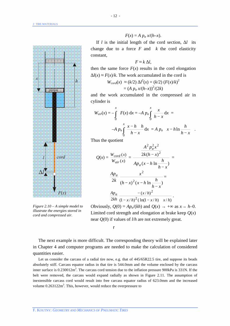
Figure 2.10 – A simple model to illustrate the energies stored in cord and compressed air.
F(x) = A pa x/(h–x). If l is the initial length of the cord section, ∆l its change due to a force F and k the cord elasticity constant,
F ≈ k ∆l, then the same force F(x) results in the cord elongation ∆l(x) ≈ F(x)/k. The work accumulated in the cord is
Wcord(x) ≈ (k/2) ∆l2(x) = (k/2) (F(x)/k)2 = (A pa x/(h–x))2/(2k)
and the work accumulated in the compressed air in cylinder is
Wair(x) = – ∫x
0
F(x) dx = –A pa ∫ −
x
xhx
0
dx =
–A pa ∫ −+−x
xhhhx
0
dx = A pa
−−
xhhhx ln .
Thus the quotient
Q(x) = )()(
xWxW
air
cord = )ln(
)(2 2
222
xhhhxAp
xhkxpA
a
a
−−
− =
)ln()(2 2
2
xhhhxxh
xk
Apa
−−−
=
)/)/1ln(()/1(
)/(2 2
2
hxhxhxhx
khApa
+−−
− .
Obviously, Q(0) = Apa/(kh) and Q(x) → +∞ as x→ h–0. Limited cord strength and elongation at brake keep Q(x) near Q(0) if values of l/h are not extremely great.
r
The next example is more difficult. The corresponding theory will be explained later in Chapter 4 and computer programs are needed to make the calculation of considered quantities easier. Let us consider the carcass of a radial tire now, e.g. that of 445/65R22.5 tire, and suppose its beads absolutely stiff. Carcass equator radius in that tire is 544.0mm and the volume enclosed by the carcass inner surface is 0.230012m3. The carcass cord tension due to the inflation pressure 900kPa is 331N. If the belt were removed, the carcass would expand radially as shown in Figure 2.11. The assumption of inextensible carcass cord would result into free carcass equator radius of 623.0mm and the increased volume 0.263122m3. This, however, would reduce the overpressure to

- -
2 TIRE MATERIALS
F. KOUTNY: GEOMETRY AND MECHANICS OF PNEUMATIC TIRES
13
p = (998×0.230012/0.263122 – 98) = 774kPa, while the cord tension would increase to 579N. Let carcass cord be the steel cord 1 from Figure 2.9. The elongation ratio corresponding to the load 579N is λ = 1.003. For the initial carcass cord length 814.18mm the tension difference 579 – 331 = 248N would produce an increased cord length lf = 815.0mm, a new equator radius of 623.33mm and volume Vf = 0.263654m3. The total energy of the compressed air contained in the cavity of the free carcass at the isothermal expansion is defined by the volume Va annulling the overpressure 774kPa, i.e. reducing the absolute air
pressure from (774 + 98)kPa = 872kPa to 98kPa, Va = 98
98774 +Vf = 2.343331m3,
Wair = 872 000 × 0.263654 ln 98
872 = 502.534kJ.
The energy stored in the carcass corresponds to the energy spent on the volume decrement due to the cord length reduction, lc = lf /λ = 815.0/1.003 = 812.56mm. The volume V(lc) = 0.262008m3. Thus,
Wcords = 872 000 × 0.263654 × ln 262008.0263654.0
= 1.440kJ.
Figure 2.11 – Carcass meridian of the 445/65R22.5 tire.
These simple estimates show that the tire wall contribution to the total energy accumulated in the inflated tire must be expected very small. In real tire, however, the bead wire is extensible as much as the steel cords at least. Also the bead is rotated by some angle due to the tension stress in the carcass cord layer winded around the bead wire bundle (Figure 1.1). Thus, the real meridian length increments in the area beyond the rim shoulders due to inflation pressure are much greater than those we have taken into account so far.
300
350
400
450
500
550
600
650
-300 -200 -100 0 100 200 300 z, mm
r, mm
belted tire
free carcass
- -
2 TIRE MATERIALS
F. KOUTNY: GEOMETRY AND MECHANICS OF PNEUMATIC TIRES
14
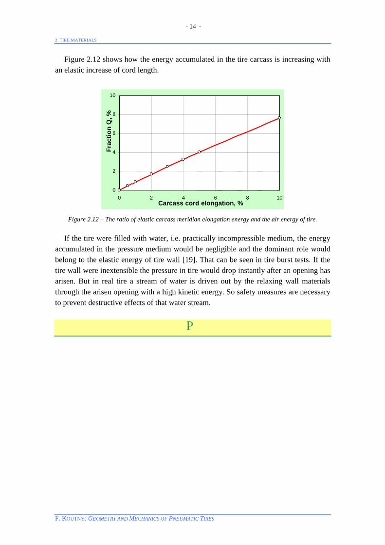
Figure 2.12 shows how the energy accumulated in the tire carcass is increasing with an elastic increase of cord length.
Figure 2.12 – The ratio of elastic carcass meridian elongation energy and the air energy of tire.
If the tire were filled with water, i.e. practically incompressible medium, the energy accumulated in the pressure medium would be negligible and the dominant role would belong to the elastic energy of tire wall [19]. That can be seen in tire burst tests. If the tire wall were inextensible the pressure in tire would drop instantly after an opening has arisen. But in real tire a stream of water is driven out by the relaxing wall materials through the arisen opening with a high kinetic energy. So safety measures are necessary to prevent destructive effects of that water stream.
P
0
2
4
6
8
10
0 2 4 6 8 10 Carcass cord elongation, %
Frac
tion
Q, %
- -
3 DIAGONAL CARCASS GEOMETRY
F. KOUTNY: GEOMETRY AND MECHANICS OF PNEUMATIC TIRES
15
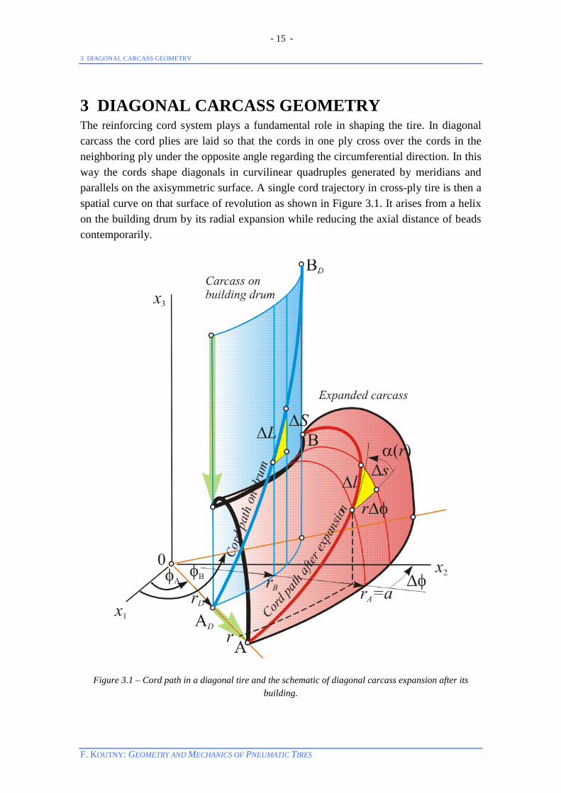
3 DIAGONAL CARCASS GEOMETRY The reinforcing cord system plays a fundamental role in shaping the tire. In diagonal carcass the cord plies are laid so that the cords in one ply cross over the cords in the neighboring ply under the opposite angle regarding the circumferential direction. In this way the cords shape diagonals in curvilinear quadruples generated by meridians and parallels on the axisymmetric surface. A single cord trajectory in cross-ply tire is then a spatial curve on that surface of revolution as shown in Figure 3.1. It arises from a helix on the building drum by its radial expansion while reducing the axial distance of beads contemporarily.
Figure 3.1 – Cord path in a diagonal tire and the schematic of diagonal carcass expansion after its building.
- -
3 DIAGONAL CARCASS GEOMETRY
F. KOUTNY: GEOMETRY AND MECHANICS OF PNEUMATIC TIRES
16
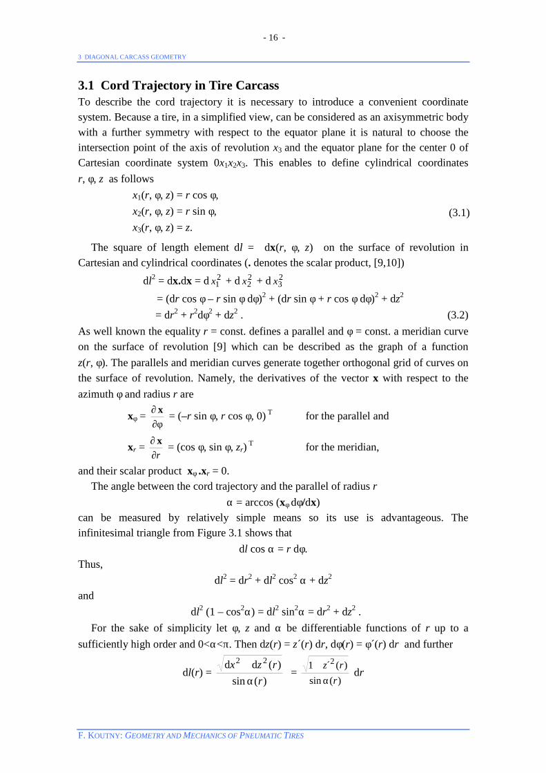
3.1 Cord Trajectory in Tire Carcass To describe the cord trajectory it is necessary to introduce a convenient coordinate system. Because a tire, in a simplified view, can be considered as an axisymmetric body with a further symmetry with respect to the equator plane it is natural to choose the intersection point of the axis of revolution x3 and the equator plane for the center 0 of Cartesian coordinate system 0x1x2x3. This enables to define cylindrical coordinates r, φ, z as follows
x1(r, φ, z) = r cos φ, x2(r, φ, z) = r sin φ, x3(r, φ, z) = z.
(3.1)
The square of length element dl = dx(r, φ, z) on the surface of revolution in Cartesian and cylindrical coordinates (. denotes the scalar product, [9,10]) dl2 = dx.dx = d 2
1x + d 22x + d 2
3x = (dr cos φ – r sin φ dφ)2 + (dr sin φ + r cos φ dφ)2 + dz2
= dr2 + r2dφ2 + dz2 . (3.2) As well known the equality r = const. defines a parallel and φ = const. a meridian curve on the surface of revolution [9] which can be described as the graph of a function z(r, φ). The parallels and meridian curves generate together orthogonal grid of curves on the surface of revolution. Namely, the derivatives of the vector x with respect to the azimuth φ and radius r are
xφ = φ∂
∂ x = (–r sin φ, r cos φ, 0) T for the parallel and
xr = r∂
∂ x = (cos φ, sin φ, zr) T for the meridian,
and their scalar product xφ .xr = 0. The angle between the cord trajectory and the parallel of radius r
α = arccos (xφ dφ/dx) can be measured by relatively simple means so its use is advantageous. The infinitesimal triangle from Figure 3.1 shows that
dl cos α = r dφ. Thus,
dl2 = dr2 + dl2 cos2 α + dz2 and
dl2 (1 – cos2α) = dl2 sin2α = dr2 + dz2 . For the sake of simplicity let φ, z and α be differentiable functions of r up to a sufficiently high order and 0<α<π. Then dz(r) = z´(r) dr, dφ(r) = φ´(r) dr and further
dl(r) = )(sin
)(22
rrzx
α+ dd
= )(sin
)(´1 2
rrz
α+
dr

- -
3 DIAGONAL CARCASS GEOMETRY
F. KOUTNY: GEOMETRY AND MECHANICS OF PNEUMATIC TIRES
17
Putting this into Equation (3.2) gives
)(sin)(´1
2
2
rrz
α
+ dr2 = dr2 + r2dφ2 + z´2 (r) dr2 ,
and by simple rearrangement one obtains
dφ(r) = )(tan)(´1 2
rrrz
α+
dr .
The total length of the spatial curve and the azimuth angle between the endpoints A, B (Figure 3.1) is then
lAB = ∫ α+A
B
r
r rrz)(sin
)(´1 2dr ,
φAB = ∫ α+A
B
r
r rrrz)(tan)(´1 2
dr .
(3.3)
The derivative z´(r) for r→rA tends to infinity, −→ Arr
lim z´(r) = –∞, and both integrals
(3.3) are singular. But for rA–rB< 2R the length of the arc of the circle (r – (rA – R))2 + z2 = R2
expressed by the integral
∫ +B
A
r
r
rz )(´1 2 dr
is final evidently. The same is true also for 0<α(r)≤π/2 and any reasonable meridian curve z(r). If α(r) = π/2 (radial carcass),
lAB = ∫ +A
B
r
r
rz )(´1 2 dr , φAB = ∫A
B
r
r
0 dr = 0 .
Problems with singularity may be avoided by transforming the integrals (3.3) to line integrals of the first kind [9]. The infinitesimal length of the meridian curve is
ds(r) = )(´1 2 rz+ dr. Thus, if sAB is the total meridional length between the parallels r = rB and r = rA, then
lAB = ∫ α
ABs
sr0 ))((sin1 ds , φAB = ∫ α
ABs
srsr0 ))((tan)(1 ds . (3.4)
These formulas together with numerical computing the integrals [10] played very useful role several decades ago, because then the tires used to be given merely by its cross-sectional drawings and both values lAB, φAB had to be computed manually [20]. For example, the 3-nodal Gauss’ quadrature formula needs three radii r-1, r0, r1 shown in Figure 3.2a. This may be even simplified, when calculating over the whole meridian

- -
3 DIAGONAL CARCASS GEOMETRY
F. KOUTNY: GEOMETRY AND MECHANICS OF PNEUMATIC TIRES
18
arc as shown in Figure 3.2b (with a greater error).
Figure 3.2 – Radii used in Gauss formula for computing integrals (3.4). 3.2 Geodesic Line on the Surface of Revolution Let a convex surface of revolution be given by its meridian curve z(r) and let the shortest line connecting its two fixed endpoints be found (a tensioned fiber laid on the surface so that it goes through two given points on it). On the interval (rB, rA) of uniqueness of the functions z and φ this problem may be written as follows
lAB[φ] = ∫ φ++A
B
r
r
rrrz )(´)(´1 222 dr = ∫A
B
r
r
f (r, φ´) dr → minimum.
This is a simple problem when using the calculus of variations [9]. The corresponding Euler-Lagrange equation
φ′∂
φ′∂ ),(rfrd
d = 0
has its first integral
φ′∂φ′∂ ),(rf =
)()(´1
)(222
2
rrrz
rr
φ′++
φ′ = r l
rddφ = const.
But l
rddφ = cos α (Figure 3.1). Therefore the geodesic line on the surface of revolution
is characterized by the following equation r cos α(r) = const.
(Clairaut’s equation). The choice r = a presents the simplest case – the cylindrical surface (a circular tube) – on which the geodesic line, helix, runs under a constant elevation angle (lead). This curve was found in [9] as a solution of a problem concerning the conditioned maximum.

- -
3 DIAGONAL CARCASS GEOMETRY
F. KOUTNY: GEOMETRY AND MECHANICS OF PNEUMATIC TIRES
19
Imagine a thin elastic axisymmetric membrane (tube) and a uniform net of fibers (free cords without any rubber matrix) fixed only to two parallels in beads and otherwise freely frictionless movable on the membrane. The overpressure in the fluid within the membrane would force the cords to reshape in such a way that the volume enclosed by the membrane is maximal:
=φ′+′+∫ ∫
A
B
A
B
r
r
r
rBAldrrrrzdrrzr )()(1)( 222 → max.
Such problems, however, will be solved later in Chapter 4. 3.3 Carcass Expansion and the Angle α(r) The cord net in tire carcass on the building drum is embedded in the matrix of raw rubber compound. The expansion of raw carcass can be viewed as a radial displacement of the cord system in a very viscous liquid or something like this. Problems of this type are probably difficult to solve even today. That is why different models were set up to capture the behavior of the cord net embedded in the rubber. Ignoring the possibility of local shear displacement of cord plies there are two extreme cases to distinguish: § If the cord length has to be preserved, which is in full accord with reality, the
cord net is modeled locally as a combination of two systems of parallel rods connected together in fixed joints (Figure 3.3).
§ Between every two parallel rods is an incompressible material and the distance between neighboring cords in the corresponding layer must be preserved, i.e. joints must be displaced (Figure 3.4).
Figure 3.3 – Pantographic model of the carcass cord net.

- -
3 DIAGONAL CARCASS GEOMETRY
F. KOUTNY: GEOMETRY AND MECHANICS OF PNEUMATIC TIRES
20
Figure 3.4 – An element of the cord net. In the first case the distances ∆l between the neighboring nodes of parallelepipeds are constant, which implies
∆l = r ∆φ / cos α(r) = rD ∆φ / cos αD , i.e.
rr)(cos α =
D
Dr
r )(cos α = const. (cos)
This is the traditionally used cosine or pantographic rule. The area of one parallelepiped of the net is
A(α) = ∆l2 sin (2α) . This means that A tends to 0 if α→0+ as indicated in the lower part of Figure 3.3. The maximum expansion ratio is then r/rD = 1/cos αD and cos α(rD /cos αD) = 1. One can, however, suppose that the rubber matrix surrounding cords would resist such squeezing out. The distance of two neighboring cords is (Figure 3.4)
d(r) = 2r ∆φ sin α(r). The assumption d(r) = const. leads to the following equations
d(r) = 2r ∆φ sin α(r) = 2rD ∆φ sin αD = d(rD), i.e.
r sin α(r) = rD sin αD = const. (sin) This is the so called sine rule [21]. Requirement of preserving the area A(α) is a compromise between those extreme cases. The distance ∆l between two neighboring nodes on the same cord is now variable but the area A can be expressed by diagonals in the parallelepiped in Figure 3.4. The horizontal diagonal uh = 2r ∆φ, the vertical one uv = uh tan α, therefore
A(α(r)) = 21 uv uh =
21 (2r ∆φ)2 tan α(r) = 2 (rD ∆φ)2 tan αD = const.
Then r2 tan α(r) = rD
2 tan αD = const. (tan) This may be called the tangent rule. Another compromise rule is the generalized cosine rule

- -
3 DIAGONAL CARCASS GEOMETRY
F. KOUTNY: GEOMETRY AND MECHANICS OF PNEUMATIC TIRES
21
cos α(r) = E
Drr
cos αD . (E)
It comprises as special cases either E = –1, i.e. the Clairaut’s relation for geodesic line on a surface of revolution, and E = 1, i.e. the usual cosine rule.
Figure 3.5 – Comparison of angles α(r) computed with the mentioned rules to the measured values in a
strip cut of two raw rubberized cord plies assembled with angles αD = ±50°. Figure 3.5 shows the angles α(r) computed by the mentioned rules compared to results obtained by stretching the strip of width 0.1m made of two raw rubberized textile cord layers with angles αD = ±50°. The rule (E) with E = 0.9 fits the measured values quite well. But the straight line through the point (1, 50°),
α(r) = 50 – 52.95(r/rD – 1), fits the measured data also good and F-test [11] shows statistical equivalency of both the functions,
F =
∑
∑
=
=
α−−−
α−α
11
1
2
11
1
29.0,
))1/(95.5250(
))((
kkDk
kkkE
rr
r = 1.764155 < 3.47370 = F0.025(11, 11) .
The dependence
α(r) = αD – c(Drr – 1) (L)
can be taken as a further expansion rule, the linear rule.
15
20
25
30
35
40
45
50
1 1.1 1.2 1.3 1.4 1.5 r/rD
α(r), deg.
cos, E=1 sin tan E = 0.9 E = 0.8 Experiment
- -
3 DIAGONAL CARCASS GEOMETRY
F. KOUTNY: GEOMETRY AND MECHANICS OF PNEUMATIC TIRES
22
Though the radial tires are clearly dominant today, the description of crossed cord systems deserves some attention. Belts of radial tires are still built as diagonal systems and it is important to realize that a small expansion at angles round 20° introduces the reduction of width of the corresponding ply,
DWW =
D
rαα
sin)(sin ,
which may be significant. For example if the original width is WD = 200mm, the angle αD=22° and the expansion ratio 1.02 (2 percent), then the rule (E) with E = 0.9 gives
α = arcos(1.020.9 cos(22°)) = 19.29° and
W = WD D
rαα
sin)(sin = 200
°°
22sin29.19sin = 176.4mm.
The reduction of the corresponding belt ply is therefore almost 24mm, i.e. 12 percent. 3.4 Tire Building Parameters The rubberized cord fabric is cut so that cord plies of rhomboid shape with prescribed width are prepared. The cutting angle αC is approximately equal to the angle αD (given by the angle αA on tire equator and expansion rule) but sometimes it needs to be a bit corrected, e.g. with respect to possible circumferential elongation. Another quantity that must be set up is the width WD of the building drum. It is essentially determined by the cord length lBAB = 2lAB equal to the length of the helix representing the cord path on the building drum and the angle αD :
WD ≈ 2lAB sin αD. There are several technical details concerning the shape of bead parts that must be respected in practical determining the values of αC, WD and carcass ply widths for individual tires and building drums. Mathematical analysis of relationships among the angles in tire and on the building drum, the cord elongation and the building drum width was in a more detailed way presented in [22,23]. In radial carcass there is α(r) = π/2, of course. Then, obviously, αC = αD = π/2 and WD ≈ 2lAB with respect to possible increase due tightening cords in beads.
P
4 EQUILIBRIUM SHAPE
F. KOUTNY: GEOMETRY AND MECHANICS OF PNEUMATIC TIRES
23
4 EQUILIBRIUM SHAPE So far the carcass expansion with no respect to the final shape has been dealt with. The carcass expands to a fixed shape in the vulcanization press when it is pressed against the mold surface by heating medium in the bladder within the tire cavity. If there is no outer support then the carcass itself must resist the pressure on its internal surface and change its shape in accordance with the general principle of energy minimum. The energy of inflated tire at zero velocity is composed of the elastic energy of tire wall and the energy of the air compressed in tire cavity, Epot = Eelast + Eair. It was shown in Section 2.3 that the energy Eelast can be taken negligible. Then the tire wall can be reduced to a surface of revolution whose final shape is fully determined by the carcass cord net. 4.1 Air Volume Theory of the Tire Meridian Curve We will consider the unloaded inflated tire rotating with angular velocity ω. Variable thickness and density of the tire wall is reflected in surface density ρ (kg/m2) of the surface A representing the upper half of the tire (z ≥ 0). Let P be a point on A. The kinetic energy of the whole surface is
Ekin = 22
2ω ∫A
ρ(P) r2(P) dA(P) .
Let the rotating tire be considered as an energetically closed system. The surface A in cylindrical coordinates is expressed by a function
z = f(r, φ). Local measuring lengths and angles a point P of the surface is performed in tangential plane at this point, i.e. in the plane determined by two independent tangential vectors at that point [9]. The square of the length element is
dl2 = grr dr2 + gφφ dφ2 + 2 grφ dr dφ ,
where g =
φφφ
φgggg
rrrr is the local metric tensor.
In the case of axial symmetry with respect to the axis 0z the surface is given completely by its meridian curve z = f(r). Using (3.2) gives
grr = 1 + f ´2(r), grφ = 0, gφφ = r2. Thus,
dA(r, φ) = 2φφφ − rrr ggg dr dφ = 22 ))(1( rrf ′+ dr dφ = r )(1 2 rf ′+ dr dφ
and
Ekin = ω2 ∫π× )2,0(),( AB rr
ρ(r, φ) r2 r )(1 2 rf ′+ dr dφ = ω2 ∫
A
B
r
r∫π2
0
ρ(r, φ) r3 )(1 2 rf ′+ dr dφ.
4 EQUILIBRIUM SHAPE
F. KOUTNY: GEOMETRY AND MECHANICS OF PNEUMATIC TIRES
24
The mass is supposed to be distributed axisymmetrically, ρ(r, φ) = ρ(r). Due to finality of r and ρ(r) the existence of the integral on the right hand side is obvious and the Fubini theorem [9, Section 3.4] gives
Ekin[f] = 2πω2 ∫A
B
r
r
ρ(r) r3 )(1 2 rf ′+ dr .
The volume of the cavity T corresponding to the meridian curve z = f(r) is
V [f] = ∫T
dx1dx2dx3.
Transition to cylindrical coordinates and the substitution theorem [9, Section 3.4] yields
V [f] = 2 ∫Ω ),,(
),,( 321zrxxx
φ∂∂ dr dφ dz ,
where Ω = (r, φ, z) : rB < r < rA, 0 < φ < 2π, 0 < z < f(r) .
The Jacobian
),,(),,( 321
zrxxx
φ∂∂ = det
φφφ−φ
1000cossin0sincos
rr
= det
φφφ−φ
cossinsincos
rr = r.
Thus,
V [f] = 2 ∫A
B
r
r∫π2
0∫
)(
0
rfr dr dφ dz .
Using the Fubini theorem gives
V [f] = 2 ∫A
B
r
r
2π r f(r) dr = 4π ∫A
B
r
r
r f(r) dr.
The potential energy is considered equal to the energy of the air compressed in the tire cavity, i.e.
Upot[f] = p0V0 ln [ ]fVV0 = – p0V0 ln
[ ]
−−
0
01V
fVV ≈ – p0V0[ ]
−−
0
0V
fVV
= p0 [ V0 – 4 π ∫A
B
r
r
r f(r) dr] ,
where V0, p0 are the initial volume and absolute pressure, respectively. The total energy
E[f] = Ekin[f] + Upot[f] is then a functional depending on f and in real conditions E[f] is always minimized,
E[f] → min. The function f is supposed to be smooth sufficiently and satisfy conditions of preserving the following two invariants of expansion,
4 EQUILIBRIUM SHAPE
F. KOUTNY: GEOMETRY AND MECHANICS OF PNEUMATIC TIRES
25
L[f] = ∫ α
′+Ar
rBr
rf)(sin
)(1 2dr = lAB, Φ[f] = ∫ α
′+Ar
rBrr
rf)(tan
)(1 2dr = φAB. (4.1)
Search for the conditioned minimum of the energy of rotating tire may be shortly written as follows
(E[f] | L[f] = lAB, Φ[f] = φAB) → min. This is the so called isoperimetric problem with two isoperimetric restrictions [9, Chapter 6]. The standard way for its solution is based on finding a stationary point of an auxiliary functional
H = E + µL + νΦ, where µ and ν are unknown constants (Lagrange multipliers). Obviously, omitting the constant V0 and putting p = p0 one gets
H[f] = ∫A
B
r
r
h(r, f, f´) dr,
where
h(r, f, f´) = ω2ρ(r) r3 )(1 2 rf ′+ – 4πpr f + µ)(sin
)(1 2
rrf
α
′+ + ν
)(tan)(1 2
rrrf
α
′+
=
αν
+α
µ+ρω
tansin32
rr 21 f ′+ – 4πpr f.
The corresponding Euler-Lagrange equation sounds
0 = rd
d
′∂
∂fh –
fh
∂∂ =
rdd
′+
′
αν
+α
µ+ρω
232
1tansin f
fr
r + 4πpr .
Integrating this equation gives
′+
′
αν
+α
µ+ρω
232
1tansin f
fr
r = 2πp(C – r2) ,
where C is a constant. Further simplification may be attained by introducing the angle θ by equation
tan θ(r) = f ´(r). Then
αν
+α
µ+ρω
tansin32
rr sin θ(r) = 2πp(C – r2)
and
sin θ(r) =
αν
+α
µ+ρω
−π−
tansin
)(232
2
rr
Crp =
α
ν+µα
+ρω
−π−
rr
Crpcos
sin1
)(2
32
2. (4.2)
On the right side there are three constants, C, µ, ν, that are to be determined by other conditions. The function f is differentiable on (rB, rA), thus, its derivative f ´
4 EQUILIBRIUM SHAPE
F. KOUTNY: GEOMETRY AND MECHANICS OF PNEUMATIC TIRES
26
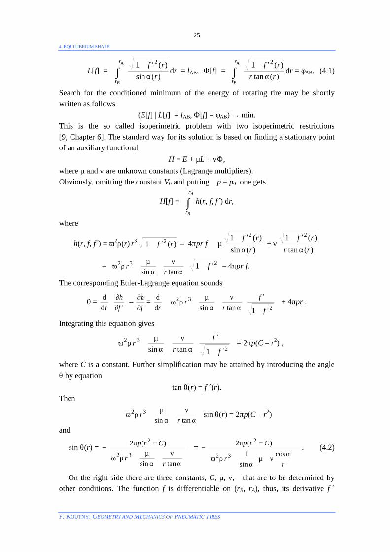
vanishes at its maximum representing the “width” W of the tire carcass (Figure 4.1). Denoting the corresponding radius rw, it is obviously f ´(rw) = 0. This implies
sin θ(rw) =
αν+µ
α+ρω
−π−
ww
w
rr
Crp
cossin
1
)(2
32
2 = 0
and C = rw
2 .
Figure 4.1 – Sketch of a typical carcass meridian curve.
The maximum radius – the upper boundary of the domain of function f is defined by the equality
θ(a) = –π/2 . This in many cases represents the carcass equator with radius a, especially in diagonal tires or in tires without belt. Then (like in Figure 4.1)
a = rA, f(a) = 0. For r = a the equation (4.2) yields
sin θ(a) =
α
ν+µα
+ρω
−π−
aaaa
rap wcos
)(sin1)(
)(2
32
22 = –1 .
From here
µ = [2πp(a2 – rw2) – ω2ρ(a) a3] sin α(a) – ν
aa)(cos α .
This and the Equation (4.2) give
sin θ(r) =
α
ν+µα
+ρω
−π−
rrrr
rrp w
cos)(sin
1)(
)(2
32
22 =
α
ν+µ+αρω
α−π−
rrrr
rrrp w
cos)(sin)(
)(sin)(2
32
22
4 EQUILIBRIUM SHAPE
F. KOUTNY: GEOMETRY AND MECHANICS OF PNEUMATIC TIRES
27
=
α
ν+α
ν−αρω−−π+αρω
α−π−
raaaaaraprrr
rrrp
w
w
cos)(cos)(sin])()(2[)(sin)(
)(sin)(2
322232
22
=
α
−α
ν+α−π+αρ−αρω
α−π−
aa
rrarapaaarrr
rrrp
w
w
)(cos)(cos)(sin)(2)](sin)()(sin)([
)(sin)(2
22332
22
.
(4.3) This general formula includes several important cases. The cosine (pantographic) expansion rule (Section 3.3) eliminates the constant ν due to its multiplication by 0, i.e. it makes the conditions (4.1) dependent ( Φ[f] = L[f] cos α(a)/a ). If in this case ω = 0 (static condition), the influence of mass distribution is annulled and one obtains the well known formula (e.g. Hofferberth [2], Biderman [3,25])
sin θ(r) =)(sin)(
)(sin)(
22
22
ara
rrr
w
w
α−
α−− .
Knowledge of the function sin θ(r) enables calculating the function f by means of numerical integration,
f(r) = f(rB) + ∫r
rB )(sin1
)(sin2 u
u
θ−
θ du
or, more generally,
f(r) = f(r0) + sign (r – r0) ∫r
r0 )(sin1
)(sin2 u
u
θ−
θ du ,
where the free integration variable (radius) is denoted by u to prevent ambiguity.
Since sin θ(a) = –1, the square root )(sin1 2 uθ− tends to 0 for u → a–. Thus, the
integral ∫r
r0
becomes singular and a special treatment is needed to compute it. The
derivative rd
d sin θ(r) is the curvature of the planar curve z = f(r) [9],
1κ(r) =rd
d sin θ(r) = rd
d21 f
f
′+
′ = 2
22
1
11
f
f
fffff
′+
′+
′′′′−′+′′
= 2/32 )1( f
f′+
′′ .
The curvature is final and different from zero. Hence, near the point r = a the function f can be approximated by the arc of its osculation circle, (a–R)2 + z2 = R2, where
R(a) = )(
11 aκ
.
The meridian curve can be computed in the two following steps:

4 EQUILIBRIUM SHAPE
F. KOUTNY: GEOMETRY AND MECHANICS OF PNEUMATIC TIRES
28
§ First a small number ε (precision) is chosen, e.g. ε=10-4, and the osculating arc z(r) = ))(2( raraR −+− over the interval [(1–ε) a, a] is constructed.
§ A decreasing sequence (1–ε)a = r0 > r1 > r2 > … > rn = rB is chosen and coordinates
zi = z(ri) = zi-1 + ∫−
i
i
r
r 1 )(sin1
)(sin2 u
u
θ−
θ du
are computed numerically (by Gauss’ 3node formula, [10]).
The distances between points should be chosen dependently on changes of f ´(r), e.g. (ri – ri-1) f ´(r i-1) ≈ const for big f ´(r i-1). More details concerning preciseness, partitioning the interval [rB, a] etc. can be found in [10, 26-30]. 4.2 Designing Problems
Figure 4.2 – A sketch of the problem (A) for a diagonal tire given through its main dimensions. Static case plays a fundamental role in attaining the given (standard) dimensions of a tire on a prescribed rim because the declared tire width and diameter are measured on inflated and unloaded tire in static condition. Subtraction of thicknesses on equator, sidewall and beads gives a, W and an arc concentric with the arc of rim shoulder on
4 EQUILIBRIUM SHAPE
F. KOUTNY: GEOMETRY AND MECHANICS OF PNEUMATIC TIRES
29
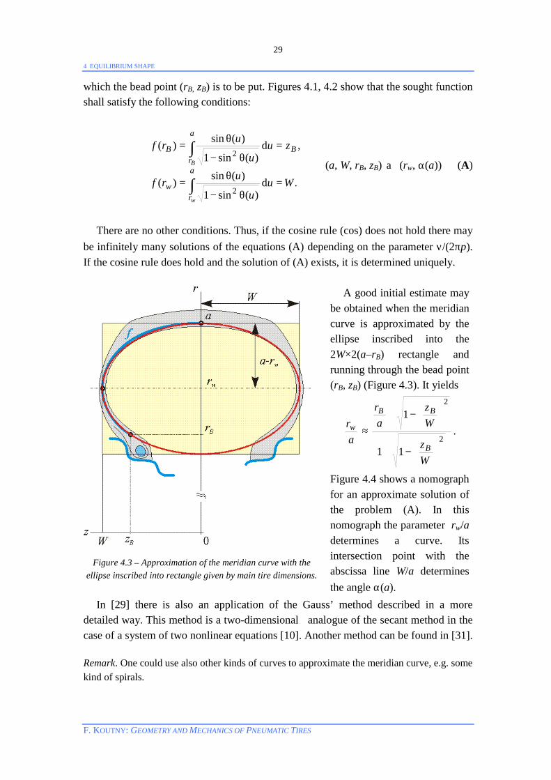
which the bead point (rB, zB) is to be put. Figures 4.1, 4.2 show that the sought function shall satisfy the following conditions:
=θ−
θ=
=θ−
θ=
∫
∫a
rw
a
rBB
w
B
Wuu
urf
zuu
urf
.)(sin1
)(sin)(
,)(sin1
)(sin)(
2
2
d
d
(a, W, rB, zB) a (rw, α(a)) (A)
There are no other conditions. Thus, if the cosine rule (cos) does not hold there may be infinitely many solutions of the equations (A) depending on the parameter ν/(2πp). If the cosine rule does hold and the solution of (A) exists, it is determined uniquely.
Figure 4.3 – Approximation of the meridian curve with the ellipse inscribed into rectangle given by main tire dimensions.
A good initial estimate may be obtained when the meridian curve is approximated by the ellipse inscribed into the 2W×2(a–rB) rectangle and running through the bead point (rB, zB) (Figure 4.3). It yields
arw ≈
2
2
11
1
−+
−+
Wz
Wz
ar
B
BB
.
Figure 4.4 shows a nomograph for an approximate solution of the problem (A). In this nomograph the parameter rw/a determines a curve. Its intersection point with the abscissa line W/a determines the angle α(a).
In [29] there is also an application of the Gauss’ method described in a more detailed way. This method is a two-dimensional analogue of the secant method in the case of a system of two nonlinear equations [10]. Another method can be found in [31]. Remark. One could use also other kinds of curves to approximate the meridian curve, e.g. some kind of spirals.
4 EQUILIBRIUM SHAPE
F. KOUTNY: GEOMETRY AND MECHANICS OF PNEUMATIC TIRES
30
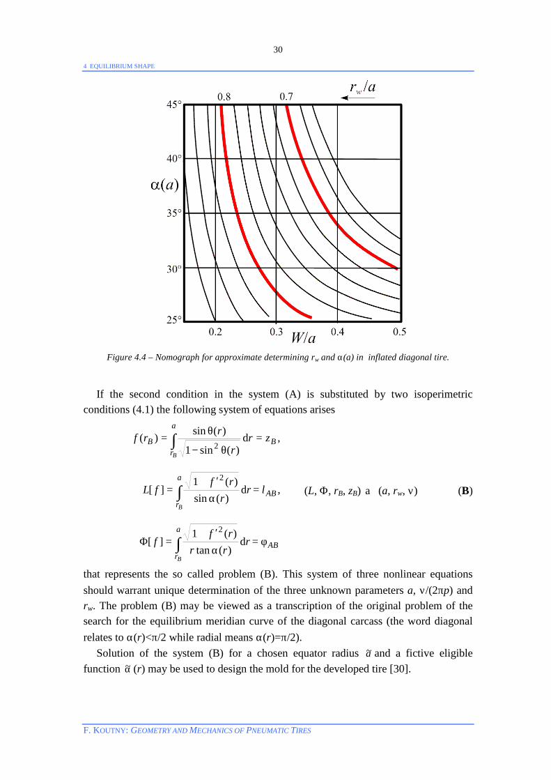
Figure 4.4 – Nomograph for approximate determining rw and α(a) in inflated diagonal tire.
If the second condition in the system (A) is substituted by two isoperimetric conditions (4.1) the following system of equations arises
φ=α
′+=Φ
=α
′+=
=θ−
θ=
∫
∫
∫
a
rAB
a
rAB
a
rBB
B
B
B
rrrrf
f
lrr
rffL
zrr
rrf
d
,d
d
)(tan)(1
][
)(sin)(1
][
,)(sin1
)(sin)(
2
2
2
(L, Φ, rB, zB) a (a, rw, ν) (B)
that represents the so called problem (B). This system of three nonlinear equations should warrant unique determination of the three unknown parameters a, ν/(2πp) and rw. The problem (B) may be viewed as a transcription of the original problem of the search for the equilibrium meridian curve of the diagonal carcass (the word diagonal relates to α(r)<π/2 while radial means α(r)=π/2). Solution of the system (B) for a chosen equator radius a~ and a fictive eligible function α~ (r) may be used to design the mold for the developed tire [30].

4 EQUILIBRIUM SHAPE
F. KOUTNY: GEOMETRY AND MECHANICS OF PNEUMATIC TIRES
31
As soon as the polar angle between both the cord ends in beads, 2φAB, is once set up on the building drum, it remains practically preserved during the next production steps and in exploitation as well. Conversely, the cord length, 2lAB, especially in nylon or polyester materials, may change due to tension induced by inflation pressure, elasticity and creep. This must be taken into account and the carcass meridian curve in mold may be computed according to the assumed reduced cord length, 2 ABl~ , and possible axial
bead displacement, zB→ Bz~ (Figure 4.5). The fixed angle φAB can be attained naturally
by reduced values of the function α(r). The radius of carcass equator remains eligible, but it is usually chosen a~ ≤a. Thus, for a given expansion rule an angle αD must be found that substitutes the unknown a in (B).
Figure 4.5 – Paths of the same carcass cord in mold and in inflated tire. Solution of problems (A) and (B) does not exist whenever one likes. Also practical computation is relatively difficult. Those problems are discussed in more detail e.g. in [29,30]. In [30] the influence of rotating velocity on the tire shape, e.g. that of mass distribution is discussed. Nevertheless, diagonal tires have turned to be rather a specialized sort of tires today. So we can abandon this topic.
4 EQUILIBRIUM SHAPE
F. KOUTNY: GEOMETRY AND MECHANICS OF PNEUMATIC TIRES
32
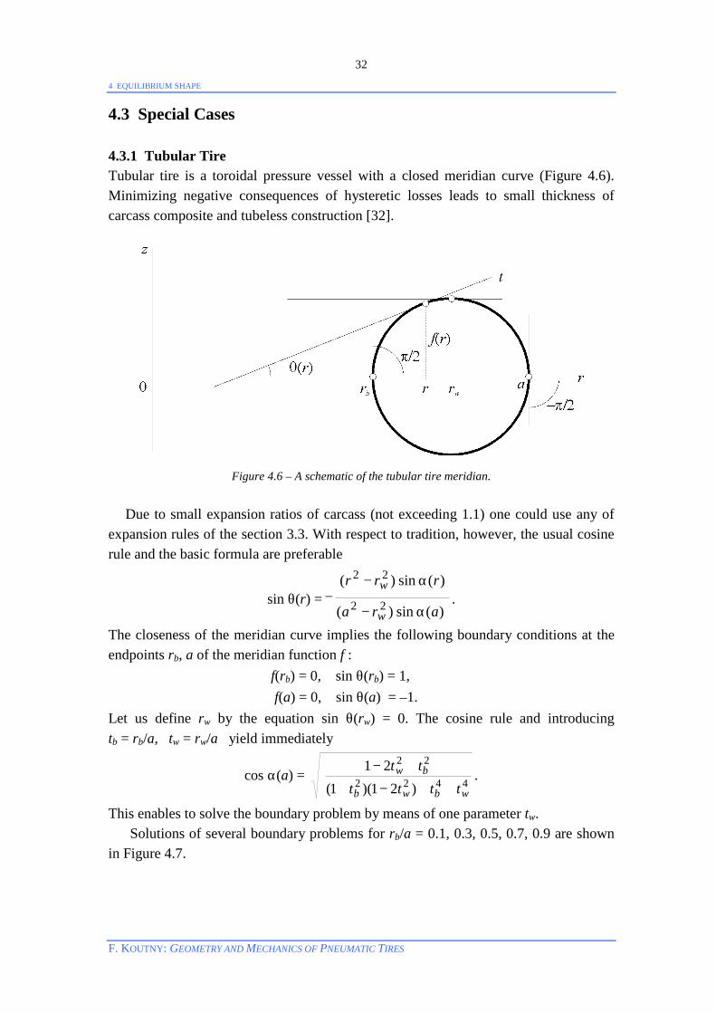
4.3 Special Cases 4.3.1 Tubular Tire Tubular tire is a toroidal pressure vessel with a closed meridian curve (Figure 4.6). Minimizing negative consequences of hysteretic losses leads to small thickness of carcass composite and tubeless construction [32].
Figure 4.6 – A schematic of the tubular tire meridian. Due to small expansion ratios of carcass (not exceeding 1.1) one could use any of expansion rules of the section 3.3. With respect to tradition, however, the usual cosine rule and the basic formula are preferable
sin θ(r) =)(sin)(
)(sin)(
22
22
ara
rrr
w
w
α−
α−− .
The closeness of the meridian curve implies the following boundary conditions at the endpoints rb, a of the meridian function f :
f(rb) = 0, sin θ(rb) = 1, f(a) = 0, sin θ(a) = –1.
Let us define rw by the equation sin θ(rw) = 0. The cosine rule and introducing tb = rb/a, tw = rw/a yield immediately
cos α(a) = 4422
22
)21)(1(21
wbwb
bw
tttttt
++−+
+− .
This enables to solve the boundary problem by means of one parameter tw. Solutions of several boundary problems for rb/a = 0.1, 0.3, 0.5, 0.7, 0.9 are shown in Figure 4.7.

4 EQUILIBRIUM SHAPE
F. KOUTNY: GEOMETRY AND MECHANICS OF PNEUMATIC TIRES
33
-0.8
-0.6
-0.4
-0.2
0
0.2
0.4
0.6
0.8
0 0.2 0.4 0.6 0.8 1
r/a
z/a
α=31.016°
α=36.276°
α=42.313°
α=47.9°
α=52.8°
Figure 4.7 – Meridians of closed toroidal cord-rubber composite membrane related to the equator
radius a and several bottom radii rb. If such a meridian curve is taken as mold profile and the angle αcord between cord and equator is chosen arbitrarily, then the equation
g(R) ≡ α(R) – arccos (aR cos αcord) = 0
defines the corresponding equator radius R after inflation. This equation must be
solved numerically [10]. R0 = cord
aaα
αcos
)(cos gives a good estimate of R.

4 EQUILIBRIUM SHAPE
F. KOUTNY: GEOMETRY AND MECHANICS OF PNEUMATIC TIRES
34
Example. Let us choose a = 330mm, rb = 305mm. The corresponding meridian curve shown in Figure 4.8 is chosen for the meridian of molded carcass. Solving the boundary problems gives: tw = 0.962135, α(a) = 53.41646°, L = 47.96014mm, Φ = 0.08662rad., V = 0.979448dm3. The cord angle for building the tubular tire is chosen αcord = 50°. Then the corresponding cord length is
Lcord = ∫ α
′+a
r cordb
rrf
)(sin)(1 2
dr = ∫ α
′+α
αa
r cordb
rrf
rr
)(sin)(1
)(sin)(sin 2
dr ≈ cord
aαα
sin)(sin L
= °
°50sin41646.53sin 47.96014mm = 50.27313mm.
-15
-10
-5
0
5
10
15
280 285 290 295 300 305 310 315 320 325 330r , mm
z , mm
Figure 4.8 – Meridian curves of molded and inflated cord-rubber composite membrane with
αcord = 50° < 53.4° = α(a). Now the new equilibrium equator radius R is to be found. It may be expected in the
neighborhood of °°
50cos53cosa ≈ 310. A simple program in DELPHI was set up to find
the equilibrium meridian curve for the couple (L, R). It gives:
R0 = 310mm → α0 = 53.199405°, g0 = –0.30091,
R1 = 315mm → α1 = 53.232299°, g1 = +0.418857. The inverse interpolation yields
R01 = 01
1gg − 11
0000
RgRg
−− = 312.09mm, g(R01) = 0.00068.
Inflated Molded
Volume V=1.010493dm3 Volume V=0.979448dm3
4 EQUILIBRIUM SHAPE
F. KOUTNY: GEOMETRY AND MECHANICS OF PNEUMATIC TIRES
35
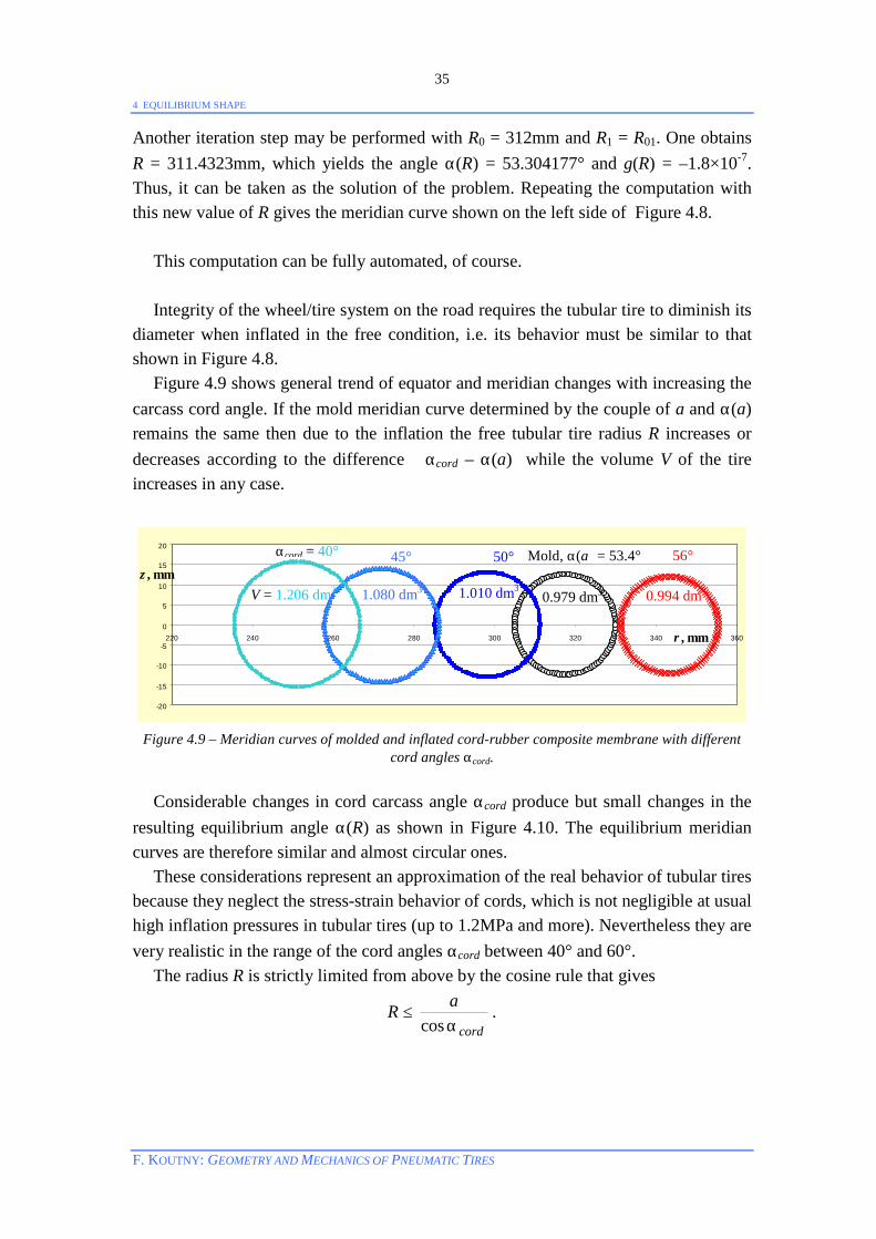
Another iteration step may be performed with R0 = 312mm and R1 = R01. One obtains R = 311.4323mm, which yields the angle α(R) = 53.304177° and g(R) = –1.8×10⁻⁷. Thus, it can be taken as the solution of the problem. Repeating the computation with this new value of R gives the meridian curve shown on the left side of Figure 4.8. This computation can be fully automated, of course. Integrity of the wheel/tire system on the road requires the tubular tire to diminish its diameter when inflated in the free condition, i.e. its behavior must be similar to that shown in Figure 4.8. Figure 4.9 shows general trend of equator and meridian changes with increasing the carcass cord angle. If the mold meridian curve determined by the couple of a and α(a) remains the same then due to the inflation the free tubular tire radius R increases or decreases according to the difference αcord – α(a) while the volume V of the tire increases in any case.
-20
-15
-10
-5
0
5
10
15
20
220 240 260 280 300 320 340 360r , mm
z , mm
Figure 4.9 – Meridian curves of molded and inflated cord-rubber composite membrane with different
cord angles αcord. Considerable changes in cord carcass angle αcord produce but small changes in the resulting equilibrium angle α(R) as shown in Figure 4.10. The equilibrium meridian curves are therefore similar and almost circular ones. These considerations represent an approximation of the real behavior of tubular tires because they neglect the stress-strain behavior of cords, which is not negligible at usual high inflation pressures in tubular tires (up to 1.2MPa and more). Nevertheless they are very realistic in the range of the cord angles αcord between 40° and 60°. The radius R is strictly limited from above by the cosine rule that gives
R ≤ cord
aαcos
.
αcord = 40° 50° 56° 45° Mold, α(a) = 53.4°
V = 1.206 dm3 1.010 dm3 1.080 dm3 0.979 dm3 0.994 dm3
4 EQUILIBRIUM SHAPE
F. KOUTNY: GEOMETRY AND MECHANICS OF PNEUMATIC TIRES
36
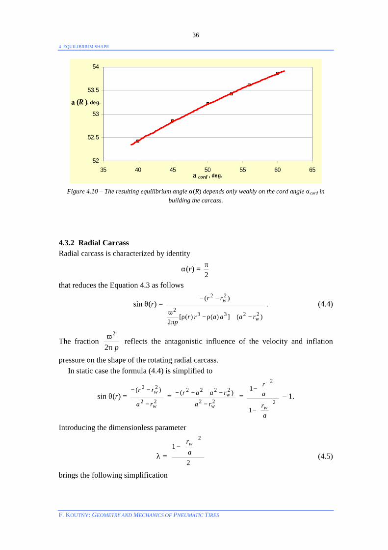
52
52.5
53
53.5
54
35 40 45 50 55 60 65α cord , deg.
α (R ), deg.
Figure 4.10 – The resulting equilibrium angle α(R) depends only weakly on the cord angle αcord in
building the carcass. 4.3.2 Radial Carcass Radial carcass is characterized by identity
α(r) = 2π
that reduces the Equation 4.3 as follows
sin θ(r) = )(])()([
2
)(
22332
22
w
w
raaarrp
rr
−+ρ−ρπ
ω
−−. (4.4)
The fraction pπ
ω2
2 reflects the antagonistic influence of the velocity and inflation
pressure on the shape of the rotating radial carcass. In static case the formula (4.4) is simplified to
sin θ(r) = 22
22 )(
w
w
ra
rr
−
−− =
22
2222 )(
w
w
ra
raar
−
−+−− = 2
2
1
1
−
−
ar
ar
w
– 1.
Introducing the dimensionless parameter
λ = 2
12
−
arw
(4.5)
brings the following simplification

4 EQUILIBRIUM SHAPE
F. KOUTNY: GEOMETRY AND MECHANICS OF PNEUMATIC TIRES
37
sin θ(r) = λ
−
2
12
ar
– 1. (4.6)
Then
f(r; a, λ) – f(a) =
−
−+
λ−−
kFEa
rSaSa
FEa
22
])1(ln21[
])21([
for
,41
,41
,41
>λ
=λ
<λ
(4.7)
where
F = F(k, φ(r)) = ∫φ
φ
φ)(
02sin
r
k 2-1
d ,
E = E(k, φ(r)) = ∫φ
φφ)(
0
2sinr
k d-1 2 ,
are elliptic integrals of the 1st and 2nd kind in Legendre’s normal form,
S = S(r) = 2
21
ar
− ,
k2 = 4λ and φ(r) = arcsin krS )( for λ <
41 ,
k2 = λ41 and φ(r) = arccos
ar for λ >
41 .
Several examples can be seen in Figure 4.11. The length l of an arc of the meridian curve over an interval [r, a] may be computed as follows [33]
l(r; a, λ) – l(a) =
λ
λ
aF
-Sa
Fa
41ln
2
)( for
.41
,41
,41
>λ
=λ
<λ
Similarly, the volume V of the corresponding cavity
V(r; a, λ) = 4π ∫a
r
r f(r; a) dr = 2π [a2f(a) – r2f(r; a) – I(r)] .
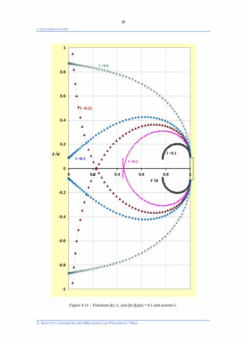
4 EQUILIBRIUM SHAPE
F. KOUTNY: GEOMETRY AND MECHANICS OF PNEUMATIC TIRES
38
-1
-0.8
-0.6
-0.4
-0.2
0
0.2
0.4
0.6
0.8
1
0 0.2 0.4 0.6 0.8 1r /a
z /a
Figure 4.11 – Functions f(r; λ, a)/a for f(a)/a = 0.1 and several λ.
λ=0.2
λ=0.1
λ=0.25
λ=0.3
λ=0.6

4 EQUILIBRIUM SHAPE
F. KOUTNY: GEOMETRY AND MECHANICS OF PNEUMATIC TIRES
39
Here, on the right side,
I(r) = ∫a
r
r2 tan θ(r) dr = a3 ∫1
ar/ )14)(1(
)21(22
22
tt
tt
+−λ−
−λ− dt
=
φ−φ
+
6/))](())(([
6/)()/21(
3
223
aHrHa
rSara for
4141
≠λ
=λ,
where
H(φ(r)) =
φ+−+−
φ+−+−
322
22
/))](()12()1([
))(()2()1(2
krJEkkF
rJEkkF for
4141
>λ
<λ
and
J(φ(r)) = k2 sin(2φ(r)) )(sin1 22 rk φ− .
Figure 4.12 shows that the theory presented here can be almost immediately used in overpressure expansion of the radial carcass in the second stage of radial tire building [34]. The basic task is to minimize the energy E needed for joining together the belt and the carcass. The shape of carcass is controlled by the distance dB between its beads, E(dB) = g(f(a; dB)). Obviously, a = const. and ∂f(a; dB)/∂dB = 0 implies dE(dB)/ddB = 0, so the width of contact area 2 f(a; dB) is to be maximized.
Figure 4.12 – Radial carcass expansion.
Cylindrical belt
Gap
Optimum bead-to-bead distance

4 EQUILIBRIUM SHAPE
F. KOUTNY: GEOMETRY AND MECHANICS OF PNEUMATIC TIRES
40
4.3.3 Isotropic Axisymmetric Linearly Elastic Membrane The meridian curve of a linearly elastic isotropic membrane can be found when solving the problem
p
−
π ∫a
rB
rrrfV
d)(2
0 + 2E
−′+∫ 00
2 )(1)( Ahrrfrrha
rB
d → min.
where V0 is an initial volume bounded by the non-extended membrane, E is the elasticity constant in Nm-2, A0 is the initial area and h is the thickness of the membrane. The membrane is supposed to expand in all directions uniformly. The additive constants do not influence the extreme behavior of the energy sum on the left side. Thus, one can introduce an energy function
F(r, f, f ´) = – 2pr f(r) + Eh(r)r )(1 2 rf ′+ . The corresponding Euler-Lagrange equation [13]
′∂
∂fF
rdd –
fF
∂∂ =
rdd (Ehr
21 f
f
′+
′) + 2pr = 0
can be easily integrated (as usual we put 21 f
f
′+
′ = sin θ)
E h(r) r sin θ + p r2 = C = const. The parameter a denotes the radius at which θ(a) = –π/2 (sin θ(a) = –1). Thus,
C = pa2 – Eha = a (pa – Eh(a)) and
sin θ(r) = rrhE
prahEpaa)())(( 2−− =
rrhErap)(
22 − – )()(
rhraha .
Let us consider the simplified case when the thickness h(r) is constant (independent of r), i.e. h(r) = h0. Then
sin θ(r) = 0Eh
pr
ra 22 − – ar /
1 = 0
2
Eahpa
arar
/)/(1 2− –
ar /1 .
If a new variable t = r/a is introduced and K = 0Eh
pa > 0 is a new constant, then
sin θ(t) = ttK 1)1( 2 −− .
Obviously, t = 1 determines the upper end of the domain of f, sin θ(1) = –1. The lower boundary of the domain of f, t = tb, is defined by sin θ(tb) = 1 for K ≥ 1 and sin θ(tb) = –1 for 0 < K < 1, i.e.
tb =
−−
1/1/11
KK for 1
1<≥
KK .
The role of the parameter K in case of fixed boundary is illustrated in Figure 4.13.

4 EQUILIBRIUM SHAPE
F. KOUTNY: GEOMETRY AND MECHANICS OF PNEUMATIC TIRES
41
0
0.5
1
1.5
2
-1.5 -1 -0.5 0 0.5 1 1.5r/r b
(z-z b )/r b
K=1.3K=1.2K=1.1K=1K=0.95K=0.9K=0.8
Figure 4.13 – Meridian curves of axisymmetric, isotropic and linearly elastic membrane. After several simple arrangements the meridian curve can be expressed by means of elliptic integrals in the following way:
f(r) = a ∫1
/ ar )(sin1
)(sin2 t
t
θ
θ
−dt = a ∫
1
/ ar22
2
1)1(1
1)1(
−−−
−−
ttK
ttK
dt
= a ∫1
/ ar ( )222
2
1)1(
1)1(
−−−
−−
tKt
tK dt = a ∫1
/ ar ))/11()(1(
)/11(222
2
Ktt
tK
−−−
−− dt.
In the important case of K > 1 (Figure 4.14) one obtains
f(r) = a [E(k, φ) – (1–1/K) F(k, φ)] , where
k = 2)/11(1 K−− = KK 12 − and φ = arcsin
−−
121 2
KtK .

4 EQUILIBRIUM SHAPE
F. KOUTNY: GEOMETRY AND MECHANICS OF PNEUMATIC TIRES
42
The special case of K = 1 yields k = 1, φ = arcsin 21 t− , i.e.
f(r) = a E(1, φ) = ∫φ
φφ−)(
0
2sin1r
d = a ∫φ
φφ)(
0
cosr
d = sin (arcsin 21 t− )
= a 21 t− . In other words, K = 1 gives f 2(r) = a2(1 – t2) = a2 – (at)2, i.e. a circle
f 2(r) + r2 = a2. This result can be obtained directly considering the curvature of the meridian curve [9]
κ(t) = a1
dtd sin θ(t) =
a1
td
d (–Kt +t
K 1−) =
a1
–K – 21
tK −
,
where K=1 implies κ(t) = a1 .
0
0.2
0.4
0.6
0.8
1
-0.6 -0.4 -0.2 0 0.2 0.4 0.6-z /a
r /a
Figure 4.14 – Meridian curves of axisymmetric, isotropic and linearly elastic membranes for several K>1.
K=5
K=3
K=1.5
K=2
4 EQUILIBRIUM SHAPE
F. KOUTNY: GEOMETRY AND MECHANICS OF PNEUMATIC TIRES
43
The behavior of the meridian curve near the lower boundary of its domain (r = atb) signalizes a loss of stability – a phenomenon that is manifested by corrugating the surface of the internal part (i.e. facing towards the axis of revolution) of free tubes when they are inflated. Another approach to the search for the shape of isotropic (flexible but inextensible) membrane or tire can be found in [35]. Remark. Considering r as a function of z, r(0) = rb, r(H) = 0 leads to the following
expression of volume V = π ∫H
0
r2 dz. Integration by parts gives
π ∫H
0
r2 dz = πr2 z 0,0
===
rHzz – 2π ∫
H
0
rz dz = – 2π ∫H
0
rz dz .
The variable z is the internal one and may therefore be denoted by r while the original r may be denoted otherwise arbitrarily. In this way we get the problem of maximizing
the standard volume integral ∫1
0
r
r
r f dr .
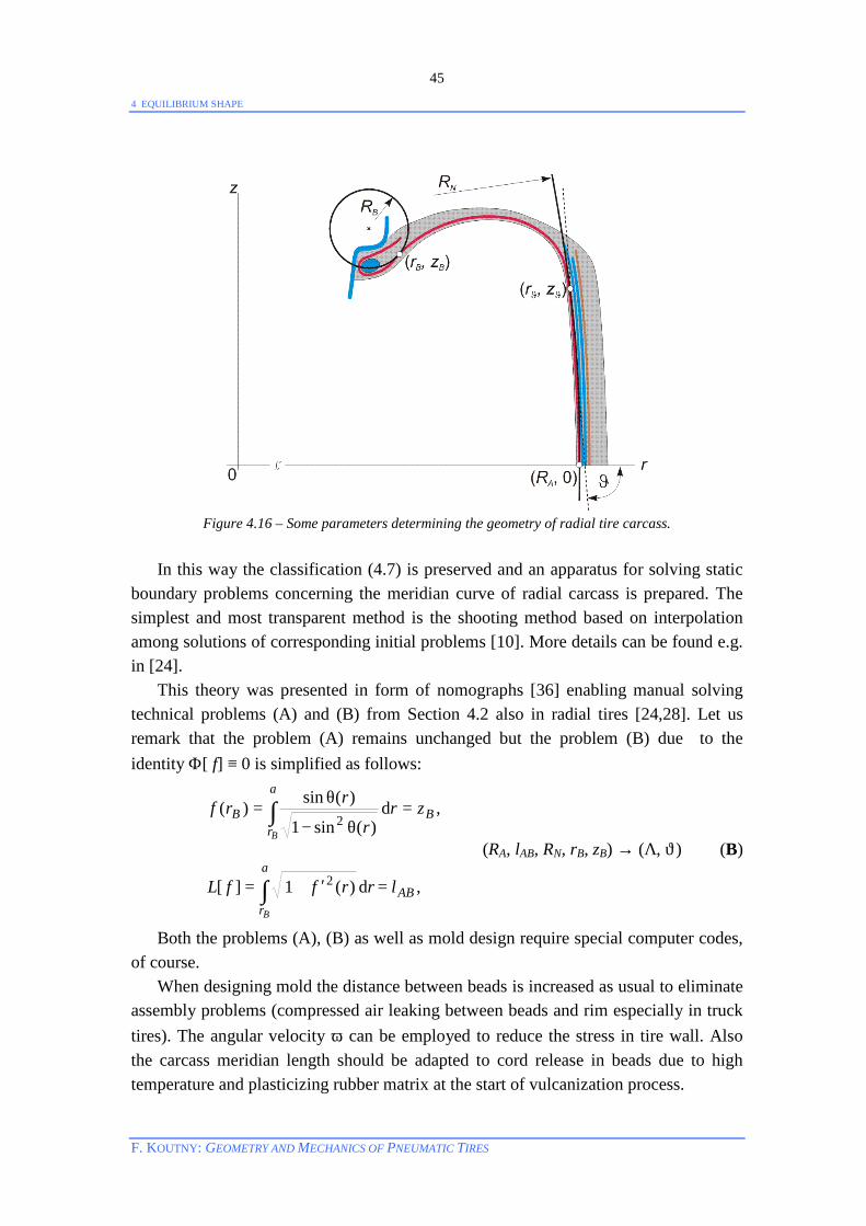
4.4 Radial Tire A schematic cross-section of the radial tire was presented in Figure 1.1 and a 3D picture of carcass expansion is shown in Figure 4.15. The belt of cord-rubber composite is a substantial element of radial tire. Its circumferential stiffness is very high while its radial bending stiffness is quite low so it behaves like a usual girdle. The belt constricts the radial expansion of tire carcass as indicated in Figure 2.11. The presence of belt as well as that of rim brings restriction conditions on the carcass meridian. They represent impenetrable areas and carcass comes in smooth contact with them, i.e. tangents of the carcass meridian and those of belt and bead area surface are identical at the borders of the contact areas [9, Section 6.4]. In first approximation the meridians of both the contact surfaces can be simply approximated by circles (Figure 4.16). Let RN be the radius of the belt circle
(r – (RA – RN))2 + z2 = RN2 ,
ϑ the absolute value of angle between the common tangent and the positive direction of the r-axis and (rϑ, zϑ) the boundary point of the contact area. Because the point (rϑ, zϑ) is unknown it is advantageous to take the angle ϑ for a new parameter. The inverse value of the product of radius rϑ and the curvature 1κ at (rϑ, zϑ) may be taken for the second parameter Λ (Figure 4.16)
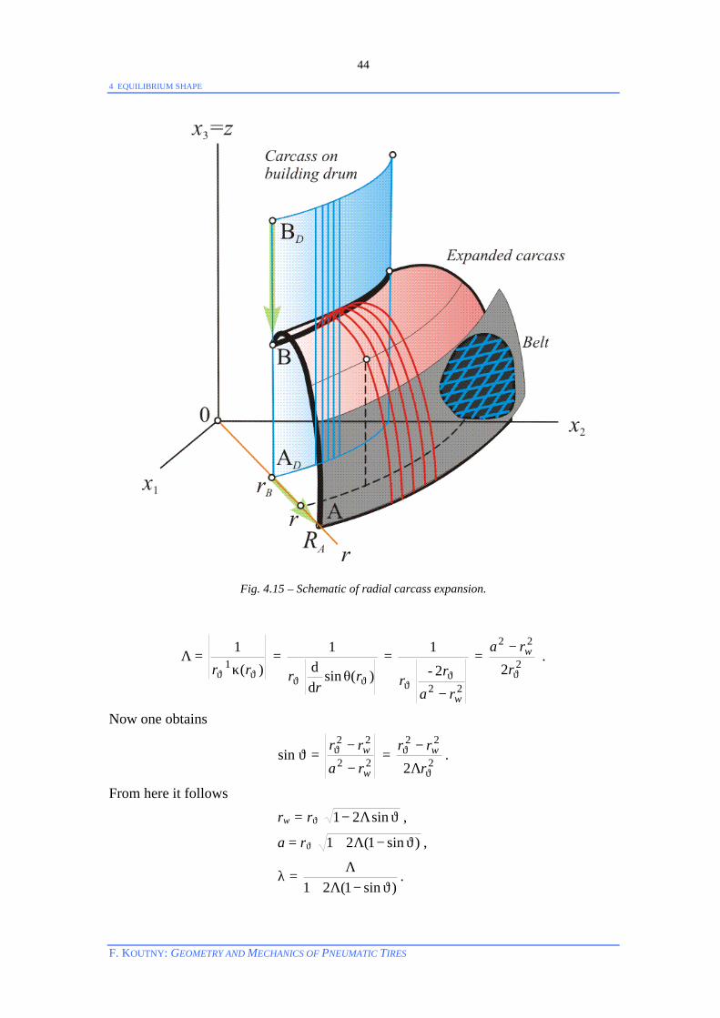
4 EQUILIBRIUM SHAPE
F. KOUTNY: GEOMETRY AND MECHANICS OF PNEUMATIC TIRES
44
Fig. 4.15 – Schematic of radial carcass expansion.
Λ = )(
11
ϑϑ κ rr =
)(sin
1
ϑϑ rr
r θdd
=
22
1
wrar
r−
ϑϑ
2- = 2
22
2 ϑ
−
rra w .
Now one obtains
sin ϑ = 22
22
w
w
rarr
−
−ϑ = 2
22
2 ϑ
ϑ
Λ
−
rrr w .
From here it follows rw = rϑ ϑΛ− sin21 ,
a = rϑ )sin1(21 ϑ−Λ+ ,
λ = )sin1(21 ϑ−Λ+
Λ .
4 EQUILIBRIUM SHAPE
F. KOUTNY: GEOMETRY AND MECHANICS OF PNEUMATIC TIRES
45
Figure 4.16 – Some parameters determining the geometry of radial tire carcass.
In this way the classification (4.7) is preserved and an apparatus for solving static boundary problems concerning the meridian curve of radial carcass is prepared. The simplest and most transparent method is the shooting method based on interpolation among solutions of corresponding initial problems [10]. More details can be found e.g. in [24]. This theory was presented in form of nomographs [36] enabling manual solving technical problems (A) and (B) from Section 4.2 also in radial tires [24,28]. Let us remark that the problem (A) remains unchanged but the problem (B) due to the identity Φ[ f] ≡ 0 is simplified as follows:
=′+=
=θ−
θ=
∫
∫
,d
d
a
rAB
a
rBB
B
B
lrrffL
zrr
rrf
)(1][
,)(sin1
)(sin)(
2
2
(RA, lAB, RN, rB, zB) → (Λ, ϑ) (B)
Both the problems (A), (B) as well as mold design require special computer codes, of course. When designing mold the distance between beads is increased as usual to eliminate assembly problems (compressed air leaking between beads and rim especially in truck tires). The angular velocity ω can be employed to reduce the stress in tire wall. Also the carcass meridian length should be adapted to cord release in beads due to high temperature and plasticizing rubber matrix at the start of vulcanization process.
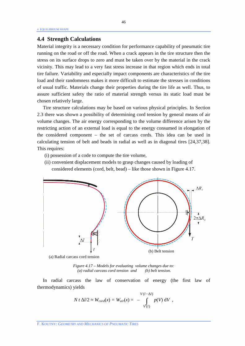
4 EQUILIBRIUM SHAPE
F. KOUTNY: GEOMETRY AND MECHANICS OF PNEUMATIC TIRES
46
4.4 Strength Calculations Material integrity is a necessary condition for performance capability of pneumatic tire running on the road or off the road. When a crack appears in the tire structure then the stress on its surface drops to zero and must be taken over by the material in the crack vicinity. This may lead to a very fast stress increase in that region which ends in total tire failure. Variability and especially impact components are characteristics of the tire load and their randomness makes it more difficult to estimate the stresses in conditions of usual traffic. Materials change their properties during the tire life as well. Thus, to assure sufficient safety the ratio of material strength versus its static load must be chosen relatively large. Tire structure calculations may be based on various physical principles. In Section 2.3 there was shown a possibility of determining cord tension by general means of air volume changes. The air energy corresponding to the volume difference arisen by the restricting action of an external load is equal to the energy consumed in elongation of the considered component – the set of carcass cords. This idea can be used in calculating tension of belt and beads in radial as well as in diagonal tires [24,37,38]. This requires:
(i) possession of a code to compute the tire volume, (ii) convenient displacement models to grasp changes caused by loading of considered elements (cord, belt, bead) – like those shown in Figure 4.17.
(a) Radial carcass cord tension
(b) Belt tension
Figure 4.17 – Models for evaluating volume changes due to: (a) radial carcass cord tension and (b) belt tension.
In radial carcass the law of conservation of energy (the first law of thermodynamics) yields
N t ∆l/2 ≈ Wcord(x) = Wair(x) = – ∫∆− )(
)(
llV
lV
p(V) dV ,
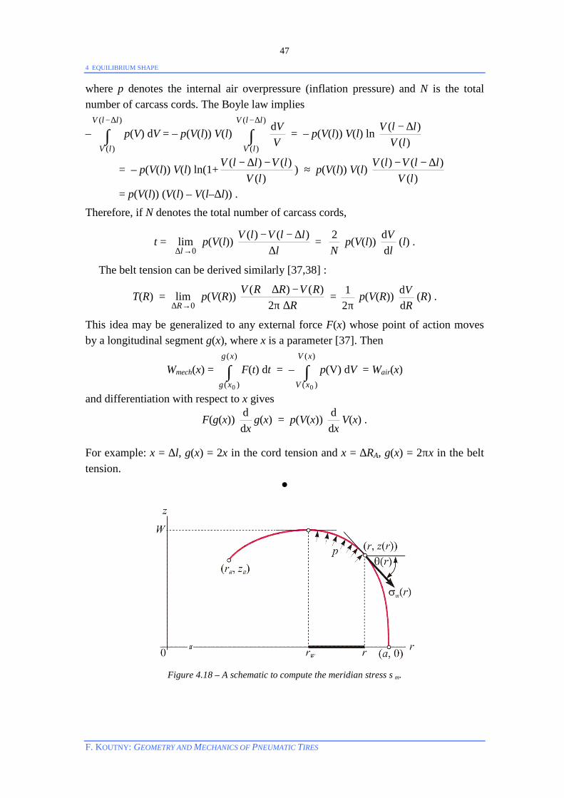
4 EQUILIBRIUM SHAPE
F. KOUTNY: GEOMETRY AND MECHANICS OF PNEUMATIC TIRES
47
where p denotes the internal air overpressure (inflation pressure) and N is the total number of carcass cords. The Boyle law implies
– ∫∆− )(
)(
llV
lV
p(V) dV = – p(V(l)) V(l) ∫∆− )(
)(
llV
lV VVd = – p(V(l)) V(l) ln
)()(
lVllV ∆−
= – p(V(l)) V(l) ln(1+)(
)()(lV
lVllV −∆− ) ≈ p(V(l)) V(l) )(
)()(lV
llVlV ∆−−
= p(V(l)) (V(l) – V(l–∆l)) .
Therefore, if N denotes the total number of carcass cords,
t = 0
lim→∆l
p(V(l)) l
llVlV∆
∆−− )()( = N2 p(V(l))
lV
dd (l) .
The belt tension can be derived similarly [37,38] :
T(R) = 0
lim→∆R
p(V(R)) R
RVRRV∆π
−∆+2
)()( = π2
1 p(V(R)) RV
dd (R) .
This idea may be generalized to any external force F(x) whose point of action moves by a longitudinal segment g(x), where x is a parameter [37]. Then
Wmech(x) = ∫)(
)( 0
xg
xg
F(t) dt = – ∫)(
)( 0
xV
xV
p(V) dV = Wair(x)
and differentiation with respect to x gives
F(g(x)) xd
d g(x) = p(V(x)) xd
d V(x) .
For example: x = ∆l, g(x) = 2x in the cord tension and x = ∆RA, g(x) = 2πx in the belt tension.
Figure 4.18 – A schematic to compute the meridian stress σm.

4 EQUILIBRIUM SHAPE
F. KOUTNY: GEOMETRY AND MECHANICS OF PNEUMATIC TIRES
48
Safe performance of tires seems to be the most probable cause of the search for the static equilibrium shape of tires as a well substantiated base for strength considerations. Figure 4.18 shows a basic schematic for computing the meridional stress σm. The z-projection of the resulting force acting on the surface area determined by parallels of radii rW and r is Fz(r) = ∫
),( rrS W
(iz. pn) dS = p ∫),( rrS W
sin (π/2 – θ(t)) dS
= p ∫π× )2,0(),( rrW
cos θ(t) t )(´1 2 tf+ dt dφ = 2π ∫r
rw
t dt = pπ(r2 – rw2),
where iz is the unit vector in the z-direction and n is the unit vector of the external normal. Because sin θ(rw) = 0 the force Fz(r) is equalized merely by the projection of total force acting on the parallel of radius r, Fz(r) = 2πr σm(r) sin θ(r). Thus,
σm(r) = )(sin2)( 22
rrrrp wθ
−.
On the other hand, in uniform radial carcass, obviously, σm(r) = n(r) t(r) , where n(r) is the number of cords per unit length segment of the r-parallel. Hence,
t(r) = )(sin)(2
)( 22
rrnrrrp wθ
− =
22
22
22
2
)(2
w
w
w
rarrN
rrp
−
−
−π =
Nrap w )( 22 −π
= const.
The relation (4.5) gives
t(r) = 2πpNa2λ = 2πp
Nr 2ϑΛ
.
The computation of belt tension T seems to be derived in the easiest way by reproducing main ideas of F. Frank [31]. The projection of pressure force acting on the contact area of belt and carcass into a meridional plane is shown in Figure 4.19. It is reduced by the meridional stress at the boundary parallel of radius rϑ. Therefore,
T = 2 p AF – 2 rϑ σm(rϑ) cos ϑ. The magnitude of the contact area projection AF can be estimated by Simpson’s formula [10],
2AF = ∫ϑ
ϑ−
z
z
r dz ≈ 6
2 ϑz [r(–zϑ) + 4r(0) + r(zϑ)] =
32 ϑz
[2r(0) + r(zϑ)].
Hence, T ≈ 2p [(2RA + rϑ) zϑ/3 – Λ rϑ
2 cos ϑ] . This total circumferential force is distributed onto individual cords corresponding to their density and angles with the circumferential direction.

4 EQUILIBRIUM SHAPE
F. KOUTNY: GEOMETRY AND MECHANICS OF PNEUMATIC TIRES
49
Figure 4.19 – Computing the total belt tension in radial tire.
Example. In 235/40R18 tire the carcass meridian curve is given as solution of the following simplified problem (A) (in mm)
(RA, W, RN, rB, zB) = (309.5, 115.5, 3000, 249.8, 104.4) → (Λ, ϑ) . This yields Λ = 0.1000949, ϑ = 1.542534, rϑ = 308.30mm, zϑ = 84.85mm and the meridional length l = lAB = 163.4mm. Let us approximate the derivative dV(l)/dl by the ratio of symmetric differences [10]
lV
dd (l) ≈
lllVllV
∆∆−−∆+
2)()( ,
where ∆l = 0.2mm. Solving the corresponding problems (B), (309.5, 163.4 ± 0.2, 3000, 249.8, 104.4) → (Λ, ϑ),
one obtains V(l+∆l) = 22.870251dm3, V(l–∆l) = 22.822429dm3. If the inflation pressure is p = 200kPa and the total number of radial cords in carcass is N = 4000, then the individual cord tension is
t = N2 p(V(l))
lV
dd (l) ≈
40002 200 000
0004.0429822022.0251870022.0 −
= 2.988875N. On the other hand,
t = 2π p Nr 2ϑΛ
≈ 40002π 200 000 × 0.1000949 × 0.30832 = 2.988883N.
Thus, the difference between the two results is negligible and caused by numerical inaccuracy. Let us remark that the real carcass is never uniform perfectly. Also cord strength is a random quantity whose distribution may be well approximated by B-distribution. More details can be found in [39].

4 EQUILIBRIUM SHAPE
F. KOUTNY: GEOMETRY AND MECHANICS OF PNEUMATIC TIRES
50
In a similar way one obtains for the belt tension
T = π2
1 p(V(R)) RV
dd (R) ≈
π2p
RRRVRRV
∆∆−−∆+
2)()(
= π2000200
0004.0022781049.0022911526.0 − = 10 383.03N
and T ≈ 2p [(2RA + rϑ) zϑ/3 – Λ rϑ
2 cos ϑ] = 2×200 000 [(2×0.3095 + 0.3083) 0.08485/3 – 0.1000949×0.30832× cos 1.542534] = 10 383.314N.
Again, both the results are practically the same and the small difference 0.31N is a consequence of rounding errors.
Remark 1. In uniform diagonal carcass the meridional stress σm(r) = n(r) t(r) sin α(r),
where r denotes the distance from the axis of revolution, n(r) is the total number of cords per unit length of r-parallel (Figures 3.3, 3.4),
n(r) = D
DDr
nrαsin
.
Here nD is the number of cords per unit length perpendicularly and αD is the cord angle on building drum (radius rD). Thus, for the usual cosine rule, cos α(r) = (r/rD) cos αD,
t(r) = )(sin)(
)(rrn
rmα
σ = p
DDD
wnr
araαα−
sin2)(sin)( 22
)(sin
12 rα
= const. ×)(sin
12 rα
.
This means: in diagonal carcass the cord tension is increasing with radius r.
Remark 2. If the bead area can be supposed stiff, the tension in wires of bead bundle may be estimated by tire volume changes due to increase of bead radius and bead displacement controlled by the shape of rim contour. Another way is using the projection of the meridional stress on radius σm(rB) into the bead plane under the angle
ϑC = arctan CB
CBrrzz
−−
, where (rC, zC) denotes the bead bundle(s) center in rim with
small conicity (5°). The total tension in bead is approximately
TC ≈ rC σm(rB) cos ϑC = rC σm(rB) 22 )()( CBCB
CB
zzrr
rr
−+−
−.
If the friction between individual wires may be supposed high enough then the force TC can be thought distributed uniformly onto individual wires and their tension confronted with their strength.
P
5 RESPONSE OF RADIAL TIRE TO EXTERNAL LOAD
F. KOUTNY: GEOMETRY AND MECHANICS OF PNEUMATIC TIRES
51
5 RESPONSE OF RADIAL TIRE TO EXTERNAL LOAD The pneumatic tire is the first dynamical element between the road and vehicle, i.e. a car, truck, aircraft, bicycle, etc. When designing a vehicle the designer needs to have some estimates of tire response to the external force signals so that he could create a tuned project. External loads in tire exploitation are non-axisymmetric which brings another complexity into tire analysis. Though the belt in radial tires restricts the carcass in radial direction it, on the other hand, has the advantage in its high circumferential stiffness. Considering negligible circumferential elongation allowed an approximation of the ´equator´ of the vertically loaded radial tire by a smooth combination of four circular arcs [12]. This model appears to be rather an artificial geometrical construction. Radial flexibility and circumferential inextensibility of the belt together with our experimental knowledge [40,41] led later to development of the so called belt model of radial tire [42]. The belt model is much more general and besides radial forces it enables to compute also lateral forces and moments in cornering tires etc. [43]. It is still relatively simple and works with analytical solutions, which provides its numerical efficiency and easy use. Also in the today’s FEM era the belt model may serve as an independent source of predictions of tire stiffness in main directions. Many experimental results have confirmed its consistency and closeness to reality. The pneumatic tire within the dynamical system of vehicle works as a spring in the first place. If m denotes the mass of the wheel (unsprung mass), t the time and x the displacement of the wheel center from its equilibrium position then according to the second law of motion (e.g. [44]) the following force F is connected with the acceleration of mass m (if m is assumed constant)
F(t) = m 2
2
tx
dd (t).
In linear spring (oscillator) this force is proportional to the displacement, F(t) = – k x(t),
where the ratio (stiffness)
k = xF .
is constant for any couple (x, F). However, the occurrence of such an ideal spring is very rare. To preserve this transparent linear model the real elastic behavior is approximated by various substitutions of the stiffness, e.g. by a local stiffness,
k(x) = xxF
dd )( .
Even an elementary knowledge on tire materials (Chapter 2) leads to expectation that the tire elasticity does also depend on temperature, velocity of deflection etc. In
5 RESPONSE OF RADIAL TIRE TO EXTERNAL LOAD
F. KOUTNY: GEOMETRY AND MECHANICS OF PNEUMATIC TIRES
52
search for logical connections one has – with some arbitrariness, of course – to summarize the important features into several clearly formulated simplifying assumptions and set up a convenient mathematical model on this basis. Dynamical behavior of the pneumatic tire is represented by the following scalar differential equation of the second order (it can be generalized to vector case easily)
2
2 )(t
txd
d = f (t, x(t), ttx
dd )( ) ,
where f is a suitable function (from the standpoint of the existence and uniqueness of solution [9,10,45]). The time dependence connected e.g. with temperature changes is ignored as usual, thus, thermodynamic equilibrium is supposed. Then the last equation may be rewritten as follows
2
2
tx
dd =
m1 (F(x) + G(x,
tx
dd )),
where the functions F, G may be simplified (linearized). The ratio G/F is very small in rolling tire. This was experimentally verified in radial oscillations in car tires [40,41].
The elastic component m
xF )( plays then a dominant role.
5.1 Static Radial Deflection Our first model that fitted experimental load–deflection curves quite well is described in [12]. The “equator” of the deflected tire is approximated by a smooth curve of the same length as the original equator of the inflated unloaded tire. This spline curve [10] is composed of four sections: the straight segment of the contact area, the large arc concentric with the original unloaded equator but with a greater radius and two equal transient arcs of smaller radius enabling a smooth joining the contact area to the free, unloaded arc. This way the radius RA is given, “bead point” (rB, zB) is kept fixed and the meridian length lAB as well as belt radius RN can be fixed or slightly changed. Thus, to any polar angle φ the following problem (B) is assigned:
(RA, lAB, RN, rB, zB)φ → (Λ, ϑ)φ . Its solution yields principally the volume VA(φ) of the corresponding axisymmetric body. The total volume of the model that belongs to the radial deflection u is then
V(u) = π21 ∫
π
π−
VA (φ) dφ = π1 ∫
π
0
VA (φ) dφ .
The last integral over the area [0, ψ] of variable radius RA(φ) is computed numerically (by the 3-node Gauss formula [10]).

5 RESPONSE OF RADIAL TIRE TO EXTERNAL LOAD
F. KOUTNY: GEOMETRY AND MECHANICS OF PNEUMATIC TIRES
53
The volume change enables to compute the energy increase of the air filling in the tire U(u). Doing this for n>3 values of ui one gets a set of points (ui, U(ui)), i = 1, …, n. It can be fitted by the following regression polynomial
P(u) = b1u2 + b2u3 . The external deflecting force F (vertical load) is then found by differentiation of P with respect to u,
F(u) = 2b1u + 3b2u2 . Direct measurement of air pressure increments in the 185SR14 radial tire at various deflections is described in [12]. There is also mentioned their comparison with corresponding predicting curve determined from volume changes of model. In this case the ratio of the air energy represents 92-95 percent of the total deflection energy. This corresponds excellently with the vertical stiffness regression published in [13] recently (as mentioned in Chapter 1). 5.2 Belt Model The ring on elastic foundations belongs to the models that are permanently used in the mechanics of tires. However, the elastic foundation created by linearly elastic spring does not describe the behavior of tires faithfully and must be improved in various ways. The belt model (Figures 1.1 and 5.1) is consistently based on the air volume work and uses the consequent theory of meridional curve (Chapter 4). Volume changes derived this way imply nonlinearity of the foundation in dependence of radial deflection. The basic theory was published in [42,43]. Here only a short survey will be given with some supplements. Figure 1.1 shows the basic partitioning the radial tire into: § low stiffness (modulus) tread area consisted of thick rubber layer equipped with
tread pattern (grooves, sipes etc.), § reinforced area of carcass, belt and beads with high stiffness in specific
directions. Equilibrium shape of the reinforced part was the theme of Chapter 4. In the foregoing Section 5.1 the volume of axisymmetric cavity swept by the meridional curve was used to compute the volume of non-axisymmetric cavity of vertically deflected tire model. The same principle creates a basis for using the elastic support that may be characterized by three coefficients of stiffness connected with axes of natural cylindrical system of coordinates 0rφz: § u = radial coordinate, ku = coefficient of radial stiffness, § v = circumferential coordinate, kv = coefficient of circumferential stiffness, § w = axial, lateral coordinate, kw = coefficient of axial, lateral stiffness.
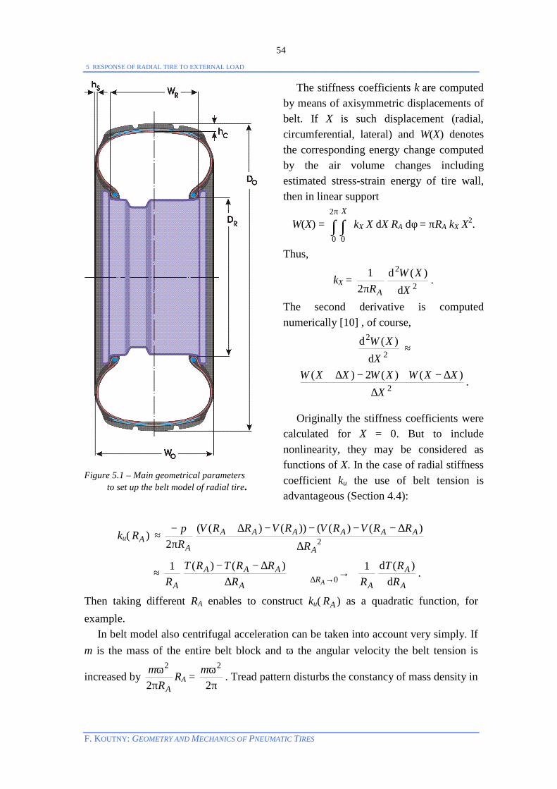
5 RESPONSE OF RADIAL TIRE TO EXTERNAL LOAD
F. KOUTNY: GEOMETRY AND MECHANICS OF PNEUMATIC TIRES
54
Figure 5.1 – Main geometrical parameters to set up the belt model of radial tire.
The stiffness coefficients k are computed by means of axisymmetric displacements of belt. If X is such displacement (radial, circumferential, lateral) and W(X) denotes the corresponding energy change computed by the air volume changes including estimated stress-strain energy of tire wall, then in linear support
W(X) = ∫ ∫π2
0 0
XkX X dX RA dφ = πRA kX X2.
Thus,
kX = ARπ2
12
2 )(X
XWd
d .
The second derivative is computed numerically [10] , of course,
2
2 )(X
XWd
d ≈
2)()(2)(
XXXWXWXXW
∆
∆−+−∆+ .
Originally the stiffness coefficients were calculated for X = 0. But to include nonlinearity, they may be considered as functions of X. In the case of radial stiffness coefficient ku the use of belt tension is advantageous (Section 4.4):
ku( AR ) ≈ AR
pπ−
2 2)()(())()((
A
AAAAAA
RRRVRVRVRRV
∆
∆−−−−∆+
≈ AR
1
A
AAAR
RRTRT∆
∆−− )()( →
→∆ 0AR
AR1
A
ARRT
dd )(
.
Then taking different RA enables to construct ku( AR ) as a quadratic function, for example. In belt model also centrifugal acceleration can be taken into account very simply. If m is the mass of the entire belt block and ω the angular velocity the belt tension is
increased by AR
mπω
2
2RA =
πω
2
2m . Tread pattern disturbs the constancy of mass density in

5 RESPONSE OF RADIAL TIRE TO EXTERNAL LOAD
F. KOUTNY: GEOMETRY AND MECHANICS OF PNEUMATIC TIRES
55
circumferential direction and small variability in belt tension along circumference certainly contributes to tire vibrations at high speeds. Hence, transversal grooves also if distributed irregularly in tread pattern [46] may turn to a source of tire noise emissions. As mentioned above, high circumferential stiffness is a characteristic property of belt of radial tire. So, in a simplified way, the belt may be considered to be inextensible longitudinally. The circumferential component of the strain tensor [47] is then
εφφ =
+
φ∂∂ uv
r1 = 0
and, because r>0, one gets a very important relationship between the radial and circumferential components of belt displacement [42]:
u = – φ∂
∂v .
Thus, the variable u is eliminated and the belt model can be described by two components of deflection, v and w.
We will shortly write v´ instead of φ∂
∂v , v´´ instead of 2
2
φ∂
∂ v , etc.
If energy losses are negligible, loading a radial tire rotating with angular velocity ω induces a deflection for which, according to the Hamilton’s principle [44], the functional
S = ∫1
0
t
t
(Ekin – Epot) dt
attains its stationary value. Here Ekin is the kinetic energy,
Ekin = πω
4
2m∫π
π−
[(RA – v´)2 + (v´´)2 + (w´´)2] dφ .
The potential energy
Epot = 2AR
∫π
π−
[Qv(v, v´, v´´) + Qw(w, w´, w´´)] dφ ,
where
Qv(v, v´, v´´) = T 2
′′
ARv + ku(v´)2 + kv v2,
Qw(w, w´, w´´) = D2
2
′′
ARw + T
2
′
ARw + kw w2,
and D is the transversal (axial) stiffness of the belt [42]. Obviously, S may be decomposed into two independent summands,
S = Sv + Sw,
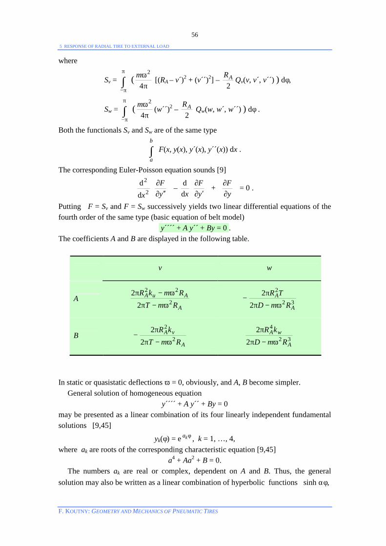
5 RESPONSE OF RADIAL TIRE TO EXTERNAL LOAD
F. KOUTNY: GEOMETRY AND MECHANICS OF PNEUMATIC TIRES
56
where
Sv = ∫π
π−
(πω
4
2m [(RA – v´)2 + (v´´)2] – 2AR Qv(v, v´, v´´) ) dφ,
Sw = ∫π
π−
(πω
4
2m (w´´)2 – 2AR Qw(w, w´, w´´) ) dφ .
Both the functionals Sv and Sw are of the same type
∫b
a
F(x, y(x), y´(x), y´´(x)) dx .
The corresponding Euler-Poisson equation sounds [9]
′′∂
∂yF
x2
2
dd –
′∂
∂yF
xdd +
∂∂
yF = 0 .
Putting F = Sv and F = Sw successively yields two linear differential equations of the fourth order of the same type (basic equation of belt model)
y´´´´ + A y´´ + By = 0 . The coefficients A and B are displayed in the following table.
v w
A A
AuA
RmTRmkR
2
22
22
ω−π
ω−π 32
2
22
A
A
RmDTRω−π
π−
B A
vA
RmTkR
2
2
22
ω−π
π− 32
4
22
A
wA
RmDkRω−π
π
In static or quasistatic deflections ω = 0, obviously, and A, B become simpler. General solution of homogeneous equation
y´´´´ + A y´´ + By = 0 may be presented as a linear combination of its four linearly independent fundamental solutions [9,45]
yk(φ) = e φka , k = 1, …, 4, where ak are roots of the corresponding characteristic equation [9,45]
a4 + Aa2 + B = 0. The numbers ak are real or complex, dependent on A and B. Thus, the general solution may also be written as a linear combination of hyperbolic functions sinh αφ,
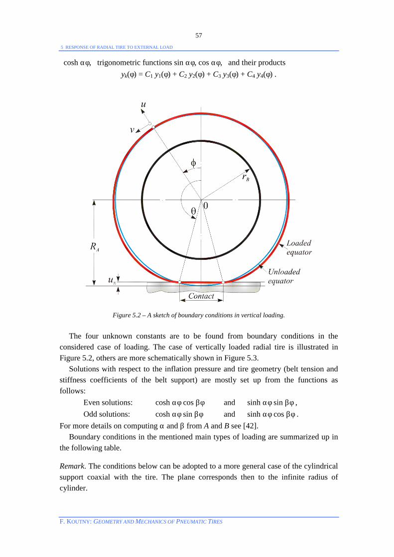
5 RESPONSE OF RADIAL TIRE TO EXTERNAL LOAD
F. KOUTNY: GEOMETRY AND MECHANICS OF PNEUMATIC TIRES
57
cosh αφ, trigonometric functions sin αφ, cos αφ, and their products yk(φ) = C1 y1(φ) + C2 y2(φ) + C3 y3(φ) + C4 y4(φ) .
Figure 5.2 – A sketch of boundary conditions in vertical loading. The four unknown constants are to be found from boundary conditions in the considered case of loading. The case of vertically loaded radial tire is illustrated in Figure 5.2, others are more schematically shown in Figure 5.3. Solutions with respect to the inflation pressure and tire geometry (belt tension and stiffness coefficients of the belt support) are mostly set up from the functions as follows:
Even solutions: cosh αφ cos βφ and sinh αφ sin βφ , Odd solutions: cosh αφ sin βφ and sinh αφ cos βφ .
For more details on computing α and β from A and B see [42]. Boundary conditions in the mentioned main types of loading are summarized up in the following table.
Remark. The conditions below can be adopted to a more general case of the cylindrical support coaxial with the tire. The plane corresponds then to the infinite radius of cylinder.
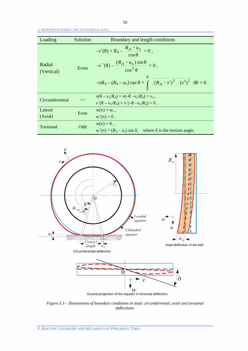
5 RESPONSE OF RADIAL TIRE TO EXTERNAL LOAD
F. KOUTNY: GEOMETRY AND MECHANICS OF PNEUMATIC TIRES
58
Loading Solution Boundary and length conditions
Radial (Vertical)
Even
–v´(θ) + RA – θ
− π
cosuRA = 0 ,
–v´´(θ) – θ
θ− π2cos
sin)( uRA = 0 ,
–πRA – (RA – uπ) tan θ + ∫θ
′′+′−0
22 )()( vvRA dθ = 0 .
Circumferential --- v(θ – vπ/RA) = v(–θ –vπ/RA) = vπ , v´(θ – vπ/RA) = v´(–θ –vπ/RA) = 0 .
Lateral (Axial)
Even w(π) = wπ , w´(π) = 0 .
Torsional Odd w(π) = 0 , w´(π) = (RA – uπ) sin δ, where δ is the torsion angle.
Circumferential deflection
Axial deflection of the belt
Ground projection of tire equator in torsional deflection.
Figure 5.3 – Illustrations of boundary conditions in static circumferential, axial and torsional
deflections.

5 RESPONSE OF RADIAL TIRE TO EXTERNAL LOAD
F. KOUTNY: GEOMETRY AND MECHANICS OF PNEUMATIC TIRES
59
If the solution vk(φ), wk(φ) is found for given deflections xk, k = 1, …, n, the corresponding energy E(xk) can be obtained by integration. Fitting the points (xk, E(xk)) by a simple function facilitates computing the load. It is advantageous, of course, to choose the regression function (regression polynomial P) as simple as possible. We have used the following polynomial of the 4th order
P(x) = x2(a1 + a2x + a3x2). Principally, three fitting polynomials Pu, Pv, Pw would be constructed for a general
deflection x =
wvu
. The force is then
F(x) =
),,(),,(),,(
wvuFwvuFwvuF
wvu
=
∂∂∂∂∂∂
wwvuPvwvuPuwvuP
wvu
/),,(/),,(/),,(
.
The belt model of the reinforced part alone (without tread layer) gives a very good approximation of vertical load-deflection curve of real radial tire. The tread layer is namely much stiffer in radial direction than the pneumatic part of tire, so the influence of tread in its serial connection to the reinforced part is small (Figure 5.4). But in tangential loadings the shear contribution of the tread to the tangential deflections is considerable. We will prefer writing (FR, FC, Fz) instead of (Fu, Fv, Fw) as a rule.
0
10
20
30
40
50
60
70
80
0 10 20 30 40 50 60
Radial deflection u, mm
Rad
ial f
orce
F, k
N
Figure 5.4 – Radial load-deflection curves in 445/65R22.5 truck tire (infl. pressure p = 800kPa).
Reinforced part
Reinforced part + tread
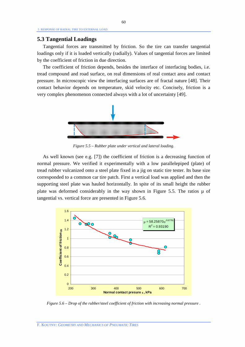
5 RESPONSE OF RADIAL TIRE TO EXTERNAL LOAD
F. KOUTNY: GEOMETRY AND MECHANICS OF PNEUMATIC TIRES
60
5.3 Tangential Loadings Tangential forces are transmitted by friction. So the tire can transfer tangential loadings only if it is loaded vertically (radially). Values of tangential forces are limited by the coefficient of friction in due direction. The coefficient of friction depends, besides the interface of interfacing bodies, i.e. tread compound and road surface, on real dimensions of real contact area and contact pressure. In microscopic view the interfacing surfaces are of fractal nature [48]. Their contact behavior depends on temperature, skid velocity etc. Concisely, friction is a very complex phenomenon connected always with a lot of uncertainty [49].
Figure 5.5 – Rubber plate under vertical and lateral loading.
As well known (see e.g. [7]) the coefficient of friction is a decreasing function of normal pressure. We verified it experimentally with a low parallelepiped (plate) of tread rubber vulcanized onto a steel plate fixed in a jig on static tire tester. Its base size corresponded to a common car tire patch. First a vertical load was applied and then the supporting steel plate was hauled horizontally. In spite of its small height the rubber plate was deformed considerably in the way shown in Figure 5.5. The ratios µ of tangential vs. vertical force are presented in Figure 5.6.
µ = 58.25870σ-0.67791
R2 = 0.93190
0
0.2
0.4
0.6
0.8
1
1.2
1.4
1.6
200 300 400 500 600 700Normal contact presure σ, kPa
Coe
ffici
ent o
f fric
tion
µ
Figure 5.6 – Drop of the rubber/steel coefficient of friction with increasing normal pressure .
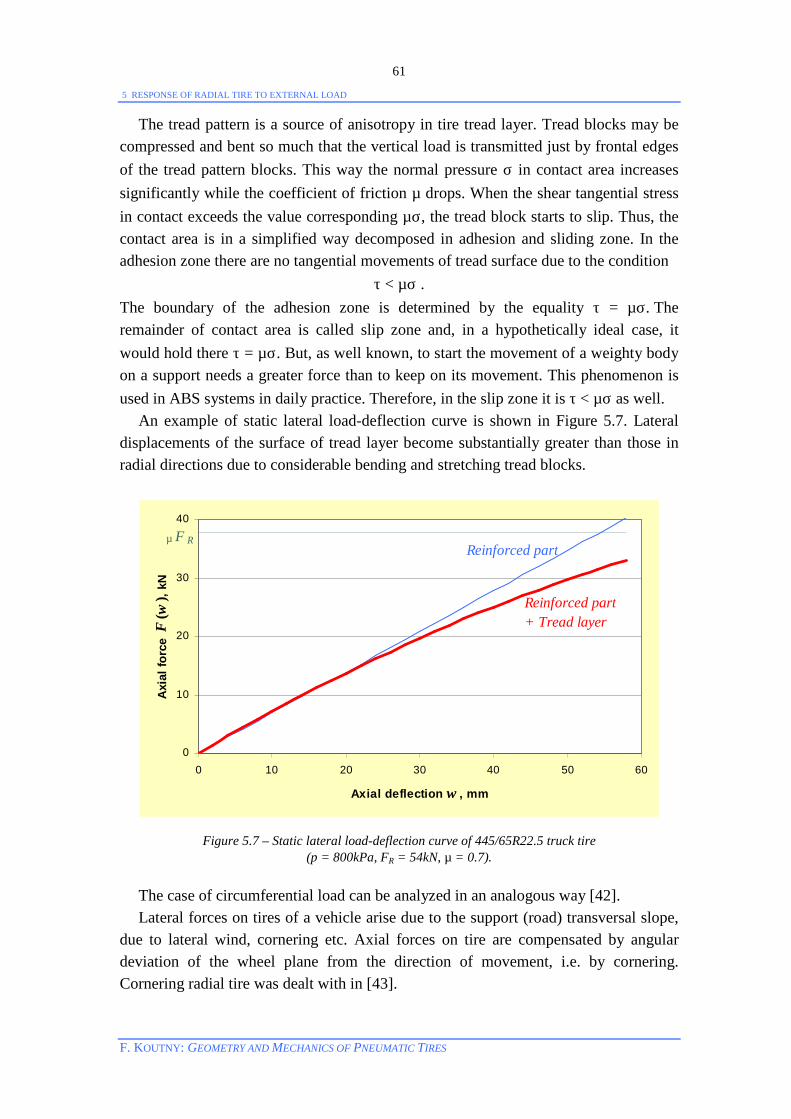
5 RESPONSE OF RADIAL TIRE TO EXTERNAL LOAD
F. KOUTNY: GEOMETRY AND MECHANICS OF PNEUMATIC TIRES
61
The tread pattern is a source of anisotropy in tire tread layer. Tread blocks may be compressed and bent so much that the vertical load is transmitted just by frontal edges of the tread pattern blocks. This way the normal pressure σ in contact area increases significantly while the coefficient of friction µ drops. When the shear tangential stress in contact exceeds the value corresponding µσ, the tread block starts to slip. Thus, the contact area is in a simplified way decomposed in adhesion and sliding zone. In the adhesion zone there are no tangential movements of tread surface due to the condition
τ < µσ . The boundary of the adhesion zone is determined by the equality τ = µσ. The remainder of contact area is called slip zone and, in a hypothetically ideal case, it would hold there τ = µσ. But, as well known, to start the movement of a weighty body on a support needs a greater force than to keep on its movement. This phenomenon is used in ABS systems in daily practice. Therefore, in the slip zone it is τ < µσ as well. An example of static lateral load-deflection curve is shown in Figure 5.7. Lateral displacements of the surface of tread layer become substantially greater than those in radial directions due to considerable bending and stretching tread blocks.
0
10
20
30
40
0 10 20 30 40 50 60
Axial deflection w , mm
Axi
al fo
rce
F(w
) , kN
µ F RReinforced part
Reinforced part+ Tread layer
Figure 5.7 – Static lateral load-deflection curve of 445/65R22.5 truck tire (p = 800kPa, FR = 54kN, µ = 0.7).
The case of circumferential load can be analyzed in an analogous way [42]. Lateral forces on tires of a vehicle arise due to the support (road) transversal slope, due to lateral wind, cornering etc. Axial forces on tire are compensated by angular deviation of the wheel plane from the direction of movement, i.e. by cornering. Cornering radial tire was dealt with in [43].

5 RESPONSE OF RADIAL TIRE TO EXTERNAL LOAD
F. KOUTNY: GEOMETRY AND MECHANICS OF PNEUMATIC TIRES
62
If the plane of wheel deviates from the instant direction of wheel movement by an angle δ (slip angle) an axial force Fz(δ), i.e. in the direction of tire revolution axis z, arises as a resultant of axial stresses τ in contact area A. The distance t between its point of action and geometric center of contact s0 of vertically loaded tire is called the pneumatic trail. Those quantities are given by the following equations
Fz = ∫∫A
τ(s, w; Fz, t) dA(s, w),
t = zF
1∫∫A
(s – s0) τ(s, w; Fz, t) dA(s, w),
where s is the circumferential and w the axial coordinate in the contact area A.
Planar support. Cylindrical segment, RD = 770mm.
Figure 5.8 – Contact areas in 15R22.5 tire. Inflation pressure p = 800kPa, vertical load 49kN.
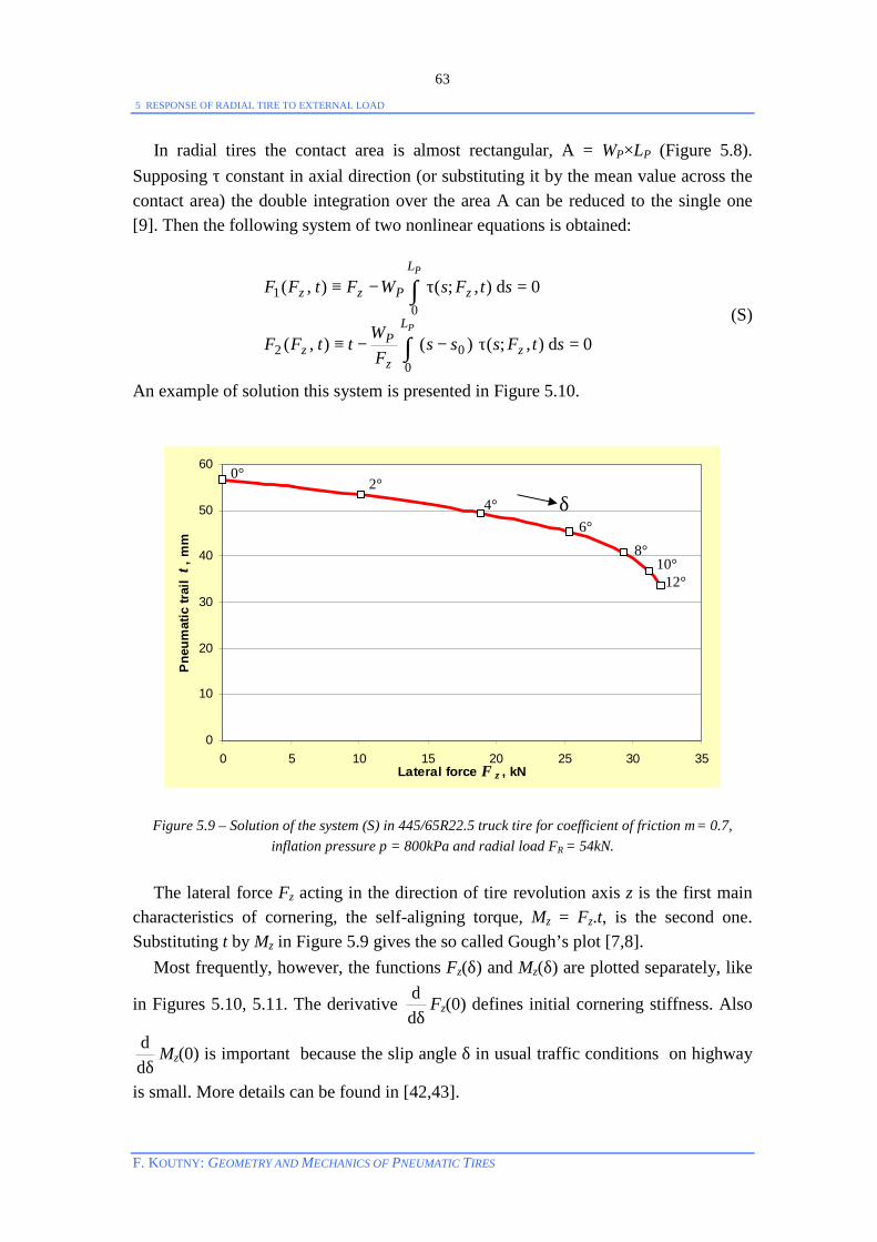
5 RESPONSE OF RADIAL TIRE TO EXTERNAL LOAD
F. KOUTNY: GEOMETRY AND MECHANICS OF PNEUMATIC TIRES
63
In radial tires the contact area is almost rectangular, A = WP×LP (Figure 5.8). Supposing τ constant in axial direction (or substituting it by the mean value across the contact area) the double integration over the area A can be reduced to the single one [9]. Then the following system of two nonlinear equations is obtained:
=τ−−≡
=τ−≡
∫
∫P
P
L
zz
Pz
L
zPzz
stFsssF
WttFF
stFsWFtFF
002
01
0),;()(),(
0),;(),(
d
d (S)
An example of solution this system is presented in Figure 5.10.
0
10
20
30
40
50
60
0 5 10 15 20 25 30 35Lateral force F z , kN
Pne
umat
ic tr
ail
t , m
m
Figure 5.9 – Solution of the system (S) in 445/65R22.5 truck tire for coefficient of friction µ = 0.7, inflation pressure p = 800kPa and radial load FR = 54kN.
The lateral force Fz acting in the direction of tire revolution axis z is the first main characteristics of cornering, the self-aligning torque, Mz = Fz.t, is the second one. Substituting t by Mz in Figure 5.9 gives the so called Gough’s plot [7,8]. Most frequently, however, the functions Fz(δ) and Mz(δ) are plotted separately, like
in Figures 5.10, 5.11. The derivative δd
d Fz(0) defines initial cornering stiffness. Also
δdd Mz(0) is important because the slip angle δ in usual traffic conditions on highway
is small. More details can be found in [42,43].
0°
δ 2°
6° 8°
12° 10°
4°
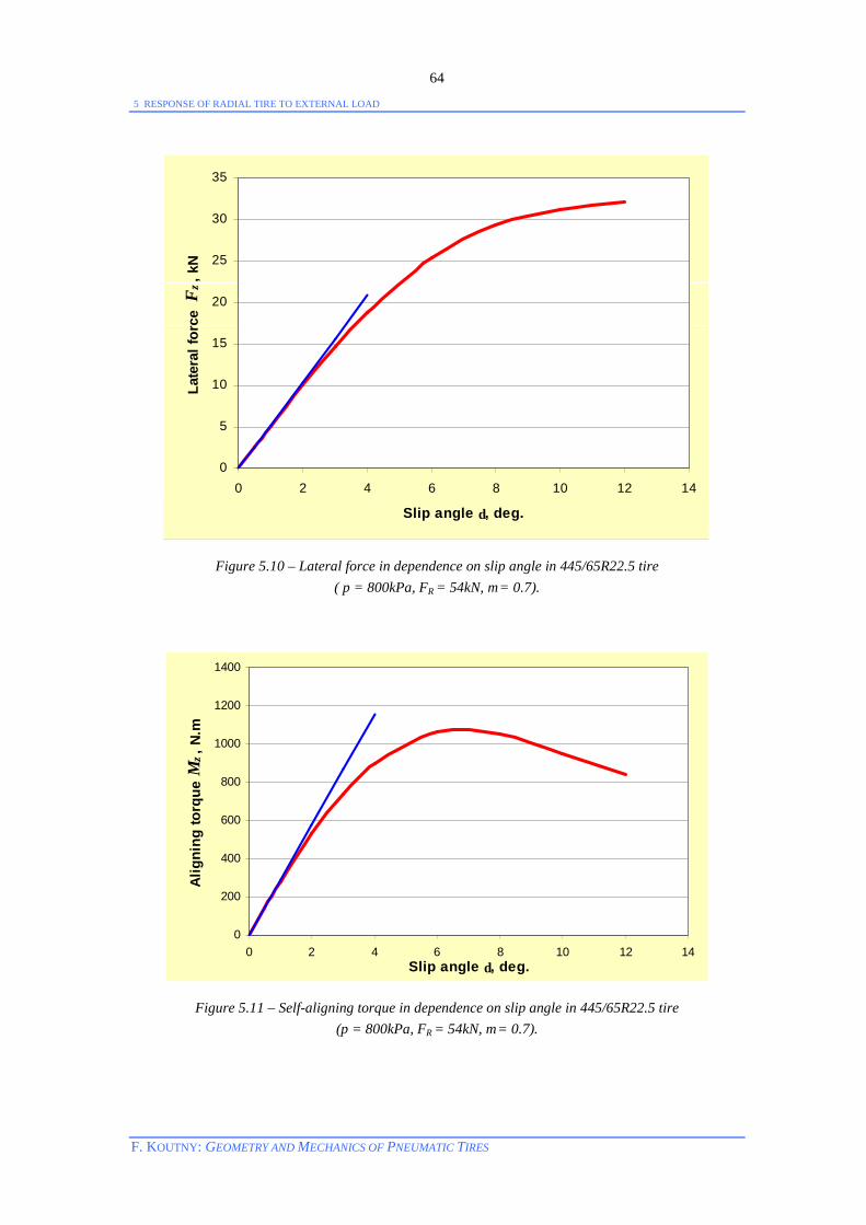
5 RESPONSE OF RADIAL TIRE TO EXTERNAL LOAD
F. KOUTNY: GEOMETRY AND MECHANICS OF PNEUMATIC TIRES
64
0
5
10
15
20
25
30
35
0 2 4 6 8 10 12 14
Slip angle δ, deg.
Late
ral f
orce
Fz,
kN
Figure 5.10 – Lateral force in dependence on slip angle in 445/65R22.5 tire ( p = 800kPa, FR = 54kN, µ = 0.7).
0
200
400
600
800
1000
1200
1400
0 2 4 6 8 10 12 14Slip angle δ, deg.
Alig
ning
torq
ue M
z, N
.m
Figure 5.11 – Self-aligning torque in dependence on slip angle in 445/65R22.5 tire (p = 800kPa, FR = 54kN, µ = 0.7).
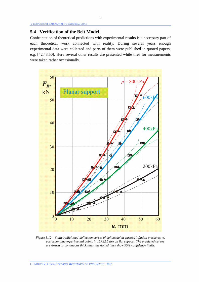
5 RESPONSE OF RADIAL TIRE TO EXTERNAL LOAD
F. KOUTNY: GEOMETRY AND MECHANICS OF PNEUMATIC TIRES
65
5.4 Verification of the Belt Model Confrontation of theoretical predictions with experimental results is a necessary part of each theoretical work connected with reality. During several years enough experimental data were collected and parts of them were published in quoted papers, e.g. [42,43,50]. Here several other results are presented while tires for measurements were taken rather occasionally.
Figure 5.12 – Static radial load-deflection curves of belt model at various inflation pressures vs. corresponding experimental points in 15R22.5 tire on flat support. The predicted curves are drawn as continuous thick lines, the dotted lines show 95% confidence limits.
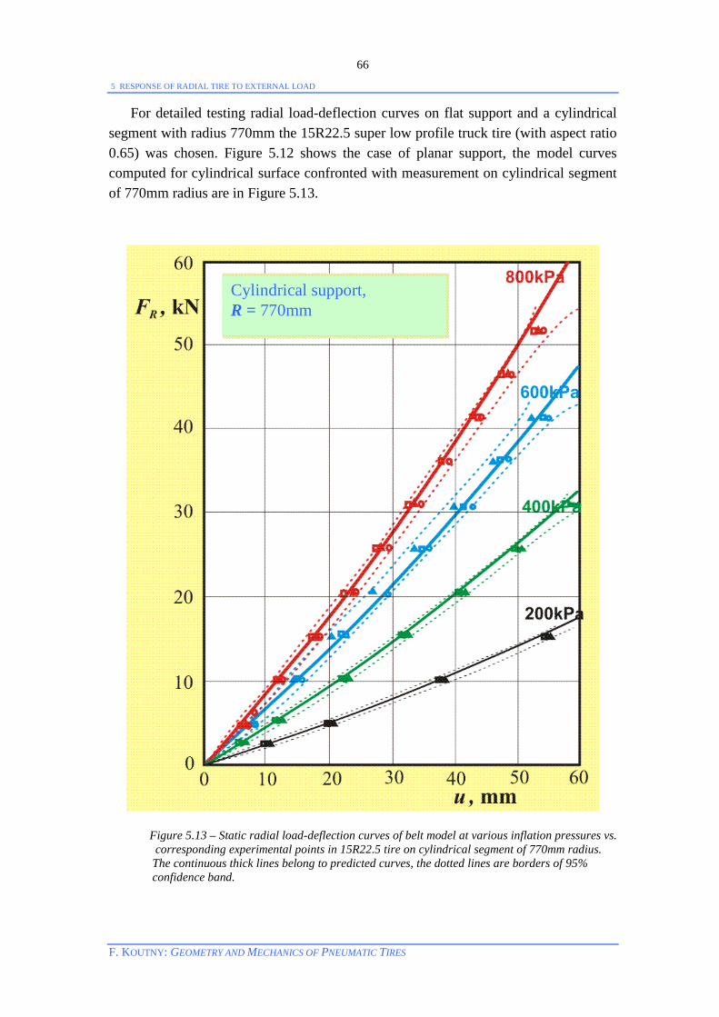
5 RESPONSE OF RADIAL TIRE TO EXTERNAL LOAD
F. KOUTNY: GEOMETRY AND MECHANICS OF PNEUMATIC TIRES
66
For detailed testing radial load-deflection curves on flat support and a cylindrical segment with radius 770mm the 15R22.5 super low profile truck tire (with aspect ratio 0.65) was chosen. Figure 5.12 shows the case of planar support, the model curves computed for cylindrical surface confronted with measurement on cylindrical segment of 770mm radius are in Figure 5.13.
Figure 5.13 – Static radial load-deflection curves of belt model at various inflation pressures vs. corresponding experimental points in 15R22.5 tire on cylindrical segment of 770mm radius. The continuous thick lines belong to predicted curves, the dotted lines are borders of 95% confidence band.
Cylindrical support, R = 770mm

5 RESPONSE OF RADIAL TIRE TO EXTERNAL LOAD
F. KOUTNY: GEOMETRY AND MECHANICS OF PNEUMATIC TIRES
67
In a smaller truck tire, 295/80R22.5, the static load-deflection curves on planar support and those on the roadwheel (D = 2m) at the speed of 100km/h are shown in Figure 5.14. The centrifugal acceleration changes the carcass meridian and reduces radial stiffness of the belt support (ku) but on the other hand the belt tension (T) is increased. At the same time the stiffness of the tread rubber decreases due to the temperature increase. These antinomy moderates the expected changes of tire stiffness at higher speeds.
Figure 5.14 – Radial load-deflection curves of belt model vs. corresponding experimental points in
295/80R22.5 tire. The predicted curves are drawn as continuous thick lines, the dotted lines belong to 95% confidence limits.
0
10
20
30
40
50
0 10 20 30 40 50 60 u , mm
F R , kN
Planar support, v = 0
Roadwheel D = 2m, v = 100km/h

5 RESPONSE OF RADIAL TIRE TO EXTERNAL LOAD
F. KOUTNY: GEOMETRY AND MECHANICS OF PNEUMATIC TIRES
68
The following Table presents laboratory measurements in 295/80R22.5 on a 2m-roadwheel at several speeds. Small variability disables to compare the results graphically.
v = 50km/h v = 100km/h v = 150km/h F, kN experiment model experiment model experiment model
3 5.0 4.4 4.63 4.7 4.0 4.53 4.1 3.4 4.31 10 14.9 14.5 14.44 14.3 13.9 14.17 13.7 13.1 13.56 15 21.4 21.0 20.92 20.6 20.3 20.59 19.9 19.5 19.78 20 27.1 26.8 27.06 26.2 26.1 26.70 25.4 25.1 25.73 25 32.8 32.6 32.91 32.0 31.9 32.53 31.1 30.9 31.44 30 38.4 38.2 38.49 37.5 37.3 38.12 36.5 36.3 36.93 35 44.0 44.0 43.84 43.2 43.1 43.48 41.9 42.0 42.23 40 49.4 49.2 48.97 48.6 48.4 48.64 47.4 47.2 47.34
In computing tangential forces one needs to know the contact length quite exactly. The comparison of predicted contact lengths to the measured ones is shown in the following Figures 5.15 and 5.16.
R2 = 0.9711
R2 = 0.9553
0
100
200
300
400
0 100 200 300 400
Measured contact length, mm
Pred
icte
d co
ntac
t len
gth,
mm
Plane
Drum, R770mm
Figure 5.15 – Contact lengths in 15R22.5 tire in radial loading.

5 RESPONSE OF RADIAL TIRE TO EXTERNAL LOAD
F. KOUTNY: GEOMETRY AND MECHANICS OF PNEUMATIC TIRES
69
Tire 15R22.5
0 50 100 150 200 250 300 350 400
(400kPa, 9.807kN)
(400kPa, 19.613kN)
(400kPa, 29.420kN)
(400kPa, 39.227kN)
(400kPa, 49.033kN)
(200kPa, 11.032kN)
(400kPa, 20.839kN)
(600kPa, 30.646kN)
(800kPa, 40.452kN)
(800kPa, 9.807kN)
(800kPa, 19.613kN)
(800kPa, 29.420kN)
(800kPa, 39.227kN)
(800kPa, 49.033kN)C
ondi
tions
(inf
latio
n pr
essu
re p
, ver
tical
load
FR
)
Contact length, mm
Plane, prediction
Plane, measurement
Drum R=770mm, pred.
Drum R=770mm, meas.
Figure 5.16 – Comparison of contact lengths in 15R22.5 tire in radial loading.
Some comparison of computed results with experimental data for circumferential and lateral loadings can be found in [42]. It is necessary to say that the measuring methods of that time were not very perfect from today’s point of view. The same could be said on cornering measurements. But this matter cannot be discussed here. Figure 5.17 illustrates dependence of lateral force and self-aligning torque on the slip angle in three car tires.
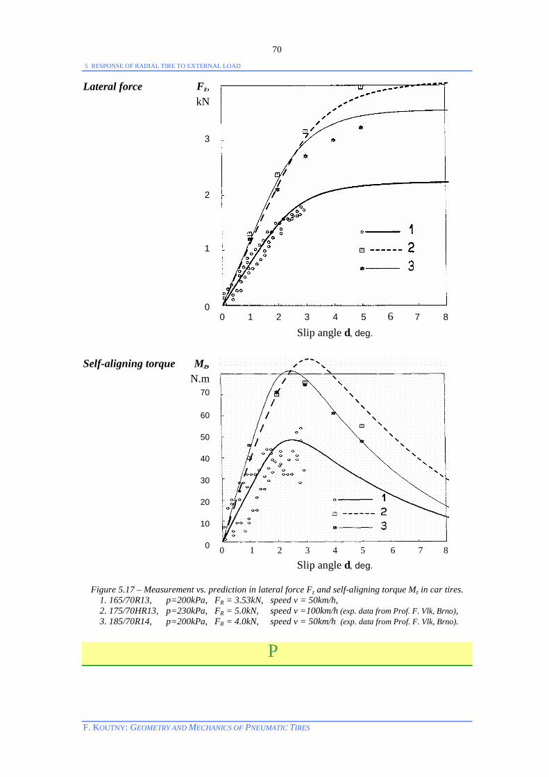
5 RESPONSE OF RADIAL TIRE TO EXTERNAL LOAD
F. KOUTNY: GEOMETRY AND MECHANICS OF PNEUMATIC TIRES
70
Lateral force Fz, kN
3
2
1
0 0 1 2 3 4 5 6 7 8
Slip angle δ, deg.
Self-aligning torque Mz, N.m
70
60
50
40
30
20
10
0 0 1 2 3 4 5 6 7 8
Slip angle δ, deg.
Figure 5.17 – Measurement vs. prediction in lateral force Fz and self-aligning torque Mz in car tires. 1. 165/70R13, p=200kPa, FR = 3.53kN, speed v = 50km/h, 2. 175/70HR13, p=230kPa, FR = 5.0kN, speed v =100km/h (exp. data from Prof. F. Vlk, Brno), 3. 185/70R14, p=200kPa, FR = 4.0kN, speed v = 50km/h (exp. data from Prof. F. Vlk, Brno).
P
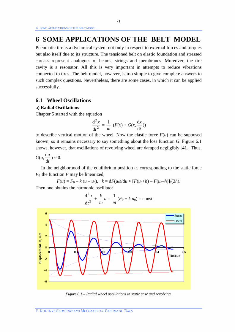
6 SOME APPLICATIONS OF THE BELT MODEL
F. KOUTNY: GEOMETRY AND MECHANICS OF PNEUMATIC TIRES
71
6 SOME APPLICATIONS OF THE BELT MODEL Pneumatic tire is a dynamical system not only in respect to external forces and torques but also itself due to its structure. The tensioned belt on elastic foundation and stressed carcass represent analogues of beams, strings and membranes. Moreover, the tire cavity is a resonator. All this is very important in attempts to reduce vibrations connected to tires. The belt model, however, is too simple to give complete answers to such complex questions. Nevertheless, there are some cases, in which it can be applied successfully. 6.1 Wheel Oscillations a) Radial Oscillations Chapter 5 started with the equation
2
2
tx
dd =
m1 (F(x) + G(x,
tx
dd ))
to describe vertical motion of the wheel. Now the elastic force F(u) can be supposed known, so it remains necessary to say something about the loss function G. Figure 6.1 shows, however, that oscillations of revolving wheel are damped negligibly [41]. Thus,
G(u,tu
dd ) ≈ 0.
In the neighborhood of the equilibrium position u0 corresponding to the static force F0 the function F may be linearized,
F(u) = F0 – k (u – u0), k = dF(u0)/du ≈ [F(u0+h) – F(u0–h)]/(2h). Then one obtains the harmonic oscillator
2
2
tu
dd +
mk u =
m1 (F0 + k u0) = const.
-6
-4
-2
0
2
4
6
0 0.1 0.2 0.3 0.4 0.5Time, s
Dis
plac
emen
t u
, mm
Static
Revol.
Figure 6.1 – Radial wheel oscillations in static case and revolving.

6 SOME APPLICATIONS OF THE BELT MODEL
F. KOUTNY: GEOMETRY AND MECHANICS OF PNEUMATIC TIRES
72
The frequency of its oscillations is
f = π21
mk .
Similar relation served for experimental establishing the “dynamical” stiffness of tires by frequency of convenient experimental system oscillations [40,41]. Predictions of
corresponding slopes uF
dd of the belt model vs. experimental results are shown in
Figure 6.2.
0
50
100
150
200
250
120 140 160 180 200 220 240 260Inflation pressure p , kPa
Dyn
amic
al s
tiffn
ess
k, k
N/m
ModelExper.
185/65 HR 14
155 SR 14
Figure 6.2 – Radial dynamical stiffness in two car tires.
If C denotes the effective rolling circumference C = 2πReff of the tire then
f = Cv
is the frequency of tire revolution (Hz). This may become the source of resonance vibrations caused by jth harmonic of uniformity disturbance, if f = fj, i.e. at the speed
vj = Cπj2
1mk =
jReff
mk , j = 1, 2, …
The most important is the highest speed. It belongs to the first harmonic
v1 = Reff mk .
Example. Figure 6.2 for the inflation pressure p = 200kPa gives the following estimates:
Tire k, kN/m m, kg Reff, m v1, km/h 155R14 155 13 0.28 110 185/65R14 180 15 0.31 122
Remark. When a tractor runs fast on the plane road low resonance speed due to low inflation pressure and thereby low stiffness of tires may cause problems.
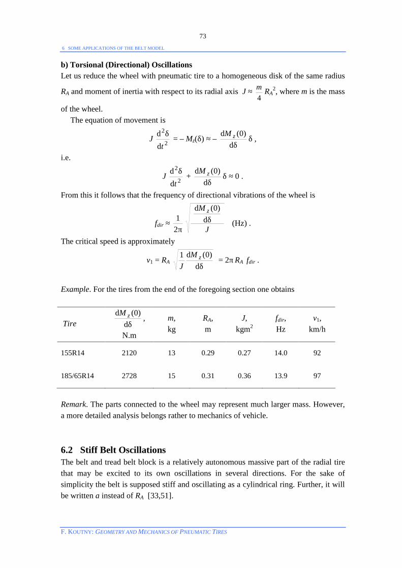
6 SOME APPLICATIONS OF THE BELT MODEL
F. KOUTNY: GEOMETRY AND MECHANICS OF PNEUMATIC TIRES
73
b) Torsional (Directional) Oscillations Let us reduce the wheel with pneumatic tire to a homogeneous disk of the same radius
RA and moment of inertia with respect to its radial axis J ≈ 4m RA
2, where m is the mass
of the wheel. The equation of movement is
J 2
2
tdd δ = – Mz(δ) ≈ –
δdd )0(zM
δ ,
i.e.
J 2
2
tdd δ +
δdd )0(zM
δ ≈ 0 .
From this it follows that the frequency of directional vibrations of the wheel is
fdir ≈ π21
J
M zδd
d )0(
(Hz) .
The critical speed is approximately
v1 = RA δd
d )0(1 zMJ
= 2π RA fdir .
Example. For the tires from the end of the foregoing section one obtains
Tire δdd )0(zM ,
N.m
m, kg
RA, m
J, kgm2
fdir, Hz
v1, km/h
155R14 2120 13 0.29 0.27 14.0 92
185/65R14 2728 15 0.31 0.36 13.9 97
Remark. The parts connected to the wheel may represent much larger mass. However, a more detailed analysis belongs rather to mechanics of vehicle. 6.2 Stiff Belt Oscillations The belt and tread belt block is a relatively autonomous massive part of the radial tire that may be excited to its own oscillations in several directions. For the sake of simplicity the belt is supposed stiff and oscillating as a cylindrical ring. Further, it will be written a instead of RA [33,51].

6 SOME APPLICATIONS OF THE BELT MODEL
F. KOUTNY: GEOMETRY AND MECHANICS OF PNEUMATIC TIRES
74
a) Radial Oscillations
It is seen in Figure 6.3 that the radial and circumferential displacements u and v with respect to the fixed rim are
u(x, φ) ≈ x sin φ, v(x, φ) ≈ x cos φ.
Potential energy corresponding to the displacement x is then
Epot ≈ 21
∫π2
0
[ku u2 + kv v2] a dφ
= ax2 ∫π
π−
2/
2/
[ku sin2φ + kv cos2φ] .
Figure 6.3 – Radial displacement of the stiff belt. Because
∫π
π−
2/
2/
sin2φ dφ = ∫π
π−
2/
2/
cos2φ dφ = 2π ,
one obtains
Epot ≈ 2π a(ku + kv) x2.
The mass of sidewalls can be neglected. If m is the mass of the belt block, then the kinetic energy of the block is
Ekin = 2m 2
tx
dd .
Considering the belt system conservative enables to use the Hamilton’s principle: the displacement x(t) gives the functional
∫t
0
L(x, tx
dd ) dt = ∫
t
0
( Ekin – Epot) dt = 21
∫t
0
[m2
tx
dd – π a x2(ku + kv) ] dt
a stationary value. The Euler-Lagrange equation [9] in this simple case yields
–xL
∂∂ +
tdd
∂
∂
tx
L
dd
= 0 = πa (ku + kv) x + m 2
2
tx
dd .
The frequency corresponding to this linear harmonic oscillator is
frad = 21
mkka vu
π+ )( (Hz) .

6 SOME APPLICATIONS OF THE BELT MODEL
F. KOUTNY: GEOMETRY AND MECHANICS OF PNEUMATIC TIRES
75
b) Torsional (Circumferential) Oscillations
Figure 6.4 shows that circumferential displacements v are the same along the whole circumference
v(φ, t) = v(t). Corresponding potential energy is
Epot = 21
∫π2
0
kv v2 a dφ = πa kv v2 ,
kinetic energy
Ekin = 2m 2
tv
dd .
Figure 6.4 – Circumferential displacement of the stiff belt. Considering the belt system conservative enables to use the Lagrange function
L(v, tv
dd ) =
2m 2
tv
dd – πa kv v2
and equation
–vL
∂∂
+ td
d
∂
∂
tv
L
dd
= 0 = πa kv v + m 2
2
tv
dd .
This yields the eigenfrequency of circumferential vibrations
fcirc = π21
makvπ2
= m
akvπ2
(Hz) .
c) Lateral (Axial) Oscillations
Axisymmetric Oscillations
Like in the case b) it is w(φ, t) = w(t) and Epot = πa kw w2, Ekin = 2m 2
tw
dd and
Esym = Epot + Ekin = πa kw w2 + 2m 2
tw
dd = const.

6 SOME APPLICATIONS OF THE BELT MODEL
F. KOUTNY: GEOMETRY AND MECHANICS OF PNEUMATIC TIRES
76
Figure 6.5 – Axisymmetric displacement
Differentiation of this equation with respect to time t gives
[ 2πa kww + m 2tw
dd2
] tw
dd = 0 ,
i.e. either tw
dd = 0 and then w = const.
is a static displacement or
2πa kww + m 2tw
dd2
= 0 ,
which yields
flat = π21
makwπ2
= m
akwπ2
(Hz) .
Antisymmetric Oscillations
Figure 6.6 – Antisymmetric displacement
In this case (Figure 6.6)
Epot = 21
∫π2
0
kw w2(t) sin2φ a dφ
= πa kw w2(t)/2,
Ekin = 21
∫π2
0 amπ2
2
tw
dd a dφ
= π2
m∫π
0
[td
d (w(t)]2 sin2φ) dφ
= 4m 2
ttw
d)(d .
Now
Epot + Ekin = 21 Esym
and the equation of movement as well as the frequency remain the same as in the axisymmetric case (Figure 6.5). But the antisymmetric oscillations (Figure 6.6) are preferable due to lower total energy.
Examples. In 165/70R13 tire we have a = 0.2685m, m = 2kg, p = 200kPa. The coefficients of stiffness and frequencies of different vibration modes are as follows:

6 SOME APPLICATIONS OF THE BELT MODEL
F. KOUTNY: GEOMETRY AND MECHANICS OF PNEUMATIC TIRES
77
v = 0km/h v = 100km/h ku, Pa 474 845 378 675 kv, Pa 322 523 318 536 kw, Pa 77 662 82 581 frad, Hz 92.3 86.3 fcirc, Hz 83.0 82.6 flat, Hz 40.7 42.0
In 235/40R18 tire a = 0.3095m, m = 5.7kg, p = 200kPa. The coefficients of stiffness and frequencies of different vibration modes are listed in the following table:
v = 0km/h v = 120km/h ku, Pa 493 020 460 834 kv, Pa 484 999 480 155 kw, Pa 116 309 124 849 frad, Hz 65.0 63.8 fcirc, Hz 64.7 64.4 flat, Hz 31.7 32.9
6.3 Incompatibility of Conditions on Road and Roadwheel Ignoring the obvious difference between road conditions and laboratory conditions concerning the heat transfer and energy dissipation one could reduce the problem of equivalent conditions to setting up equal radial deflection, contact pressure and contact length. Radial deflection is namely connected to carcass and belt deflections, contact pressure is joined with tread rubber compression and hysteresis, contact length mainly to shear stress and slips in circumferential direction. The following example shows that equivalent load and inflation pressure do not exist generally. Thus, any simulation of road regime through testing on a wheel road is necessarily unrealistic. Let us consider the 295/80R22.5 tire, for example, with inflation pressure p = 850kPa. In static condition on planar support the vertical load FR = 35kN produces radial deflection u∞ = 35.8mm, contact length LP,∞ = 232mm (Figure 5.9) and average contact pressure pm,∞ = 948kPa. Preserving those tree quantities u, LP, pm also on a roadwheel would require that the following three planar curves
u(p, FR) = u∞, LP(p, FR) = LP,∞, pm(p, FR) = pm,∞ intersect in one single point. Figure 6.7 shows these curves in the case of the considered 295/80R22.5 tire on the 2m roadwheel. An analogous picture for the 165/70R13 car tire was published in [52]. It is possible to consider more quantities, e.g. the maximum circumferential change of belt curvature represented by the carcass equator curvature at the ends of contact area.

6 SOME APPLICATIONS OF THE BELT MODEL
F. KOUTNY: GEOMETRY AND MECHANICS OF PNEUMATIC TIRES
78
0
10
20
30
40
50
60
70
0 200 400 600 800 1000 1200
Inflation pressure p , kPa
Radi
al lo
ad F
R, k
N
Figure 6.7 – Three conditions of planar contact transferred onto 2m roadwheel in 295/80R22.5 tire.
Remark. A correct formulation of the problem should be like this: what conditions in laboratory testing on drums are minimizing the differences in tire response simultaneously. So far namely only the most obvious radial deflection has been respected. 6.4 Optimization Problems First applications of mathematical models are usually connected with attempts for improvements and finding more suitable solutions of various problems in design and technology. The possibility to predict radial deflections of radial tires led to considerations on optimization (based on the theory of games) even before the belt model had been developed [53]. Some optimization examples were published also in [42,43]. Tire production necessarily follows economical interest, which, in a very simplified view, means attaining the maximum profit from a set of available raw materials. If a tire is run on highways exclusively one may suppose the tire will be exposed to smaller irregularities and deflections than somewhere off the road. So it may be designed as it would almost never be deflected more than, say, 50mm. This condition may be well fulfilled also with a tire whose total profile is just a bit higher, e.g. 100mm. Higher cross sections supply higher ride comfort and damping capacity but on the other side they can need higher material consumption.
LP = 232mm
u = 35.8mm
pm = 948kPa

6 SOME APPLICATIONS OF THE BELT MODEL
F. KOUTNY: GEOMETRY AND MECHANICS OF PNEUMATIC TIRES
79
Such conclusions, however, collide with the necessity to amortize the existing machinery in a maximum measure and in shortest time. Implementations of new ideas require investments and always bring problems. Moreover the tire and rim create one unit that must fit the system of suspension etc. Nevertheless, wide cylindrical tires with low aspect ratios on today’s vehicles show that the rational view has found its place. The influence of tire geometry on some of tire properties will be shown on the case of preserving the carcass cord length and equator radius. The diameter and width of the rim will be increased while the bead area profile will remain the same. Such changes of the main rim dimensions will then be constricted by the condition that the tangent angle θ(rB) in the bead point (Figure 4.16) is approximately 46°.
Aspect ratio
0
20
40
60
80
100
120
140
160
140 160 180 200 220 240 260 280 300r , mm
z , mm
124
7855
32
Figure 6.8 – Several meridional curves for fixed equator radius and meridional length.
The meridian curve parameters are chosen as follows: § equator radius RA =300mm, § meridian length lAB = 200mm, § bead area height rB – Drim/2 ≈ 42mm.
Other parameters are listed in the following table.
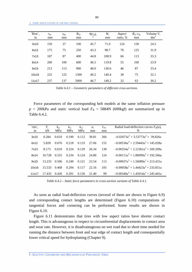
6 SOME APPLICATIONS OF THE BELT MODEL
F. KOUTNY: GEOMETRY AND MECHANICS OF PNEUMATIC TIRES
80
´Rim´, in
rB, mm
zB, mm
RN, mm
θ(rB), °
W, mm
Aspect ratio, %
RA–rB, mm
Volume V, dm3
3x10 150 37 100 45.7 71.0 124 150 24.5
6x12 175 75 250 43.3 98.7 78 125 31.9
7x13 187 87 400 44.8 108.9 66 113 33.3
8x14 200 100 600 46.5 119.8 55 100 33.9
9x15 213 113 900 48.0 130.6 46 87 33.4
10x16 225 125 1300 49.2 140.4 38 75 32.1
11x17 237 137 5000 46.7 149.2 32 63 30.2
Table 6.4.1 – Geometric parameters of different cross-sections. Force parameters of the corresponding belt models at the same inflation pressure p = 200kPa and static vertical load FR = 5884N (600kgf) are summarized up in Table 6.4.2.
´rim´, in
T, kN
ku, MPa
kv, MPa
kw, MPa
u, mm
LP, mm
Radial load-deflection curves FR(u), N
3x10 0.284 0.610 0.190 0.112 39.81 266 –0.02073u3 + 3.53773u2 + 39.826u
6x12 5.828 0.676 0.218 0.133 27.66 155 –0.00536u3 + 2.59443u2 + 145.028u
7x13 8.173 0.610 0.224 0.129 26.34 138 –0.00254u3 + 2.12361u2 + 169.209u
8x14 10.728 0.555 0.234 0.124 24.86 124 –0.00111u3 + 1.80099u2 + 192.566u
9x15 13.233 0.506 0.249 0.121 23.54 113 –0.00037u3 + 1.56089u2 + 213.431u
10x16 15.533 0.468 0.294 0.117 22.16 105 –0.00058u3 + 1.44423u2 + 233.851u
11x17 17.435 0.436 0.291 0.136 21.40 99 –0.00340u3 + 1.45014u2 + 245.441u
Table 6.4.2 – Static force parameters in cross-section variants of Table 6.4.1.
As soon as radial load-deflection curves (several of them are shown in Figure 6.9) and corresponding contact lengths are determined (Figure 6.10) computations of tangential forces and cornering can be performed. Some results are shown in Figure 6.10. Figure 6.11 demonstrates that tires with low aspect ratios have shorter contact length. This is advantageous in respect to circumferential displacements in contact area and wear rate. However, it is disadvantageous on wet road due to short time needed for running the distance between front and rear edge of contact length and consequentially lower critical speed for hydroplaning (Chapter 9).
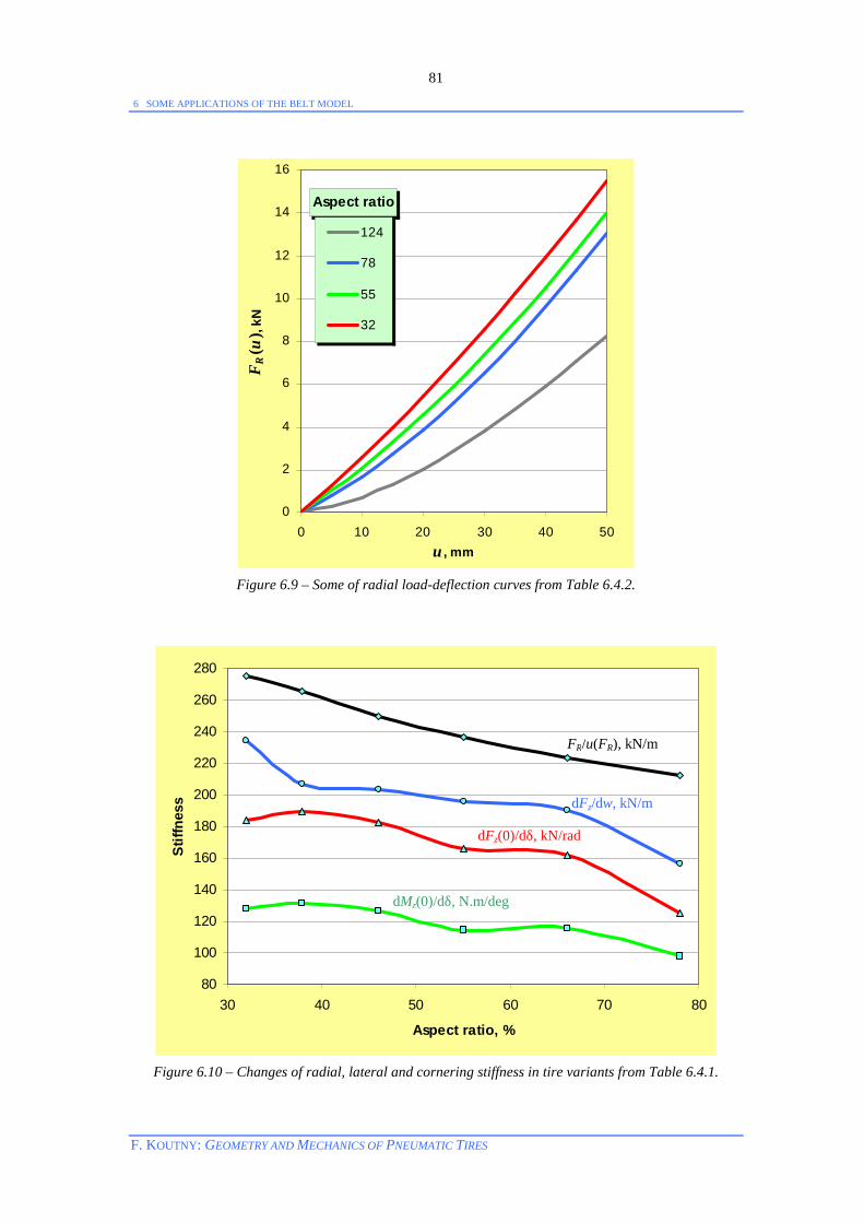
6 SOME APPLICATIONS OF THE BELT MODEL
F. KOUTNY: GEOMETRY AND MECHANICS OF PNEUMATIC TIRES
81
Aspect ratio
0
2
4
6
8
10
12
14
16
0 10 20 30 40 50u , mm
F R(u
) , kN
124
78
55
32
Figure 6.9 – Some of radial load-deflection curves from Table 6.4.2.
80
100
120
140
160
180
200
220
240
260
280
30 40 50 60 70 80
Aspect ratio, %
Stiff
ness
Figure 6.10 – Changes of radial, lateral and cornering stiffness in tire variants from Table 6.4.1.
FR/u(FR), kN/m
dFz(0)/dδ, kN/rad
dMz(0)/dδ, N.m/deg
dFz/dw, kN/m
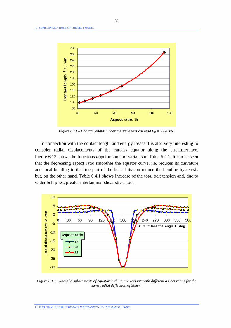
6 SOME APPLICATIONS OF THE BELT MODEL
F. KOUTNY: GEOMETRY AND MECHANICS OF PNEUMATIC TIRES
82
80
100
120
140
160
180
200
220
240
260
280
30 50 70 90 110 130
Aspect ratio, %
Cont
act l
engt
h L P
, mm
Figure 6.11 – Contact lengths under the same vertical load FR = 5.887kN.
In connection with the contact length and energy losses it is also very interesting to consider radial displacements of the carcass equator along the circumference. Figure 6.12 shows the functions u(φ) for some of variants of Table 6.4.1. It can be seen that the decreasing aspect ratio smoothes the equator curve, i.e. reduces its curvature and local bending in the free part of the belt. This can reduce the bending hysteresis but, on the other hand, Table 6.4.1 shows increase of the total belt tension and, due to wider belt plies, greater interlaminar shear stress too.
Aspect ratio
-30
-25
-20
-15
-10
-5
0
5
10
0 30 60 90 120 150 180 210 240 270 300 330 360Circumferential angle φ , deg
Rad
ial d
ispl
acem
ent
u, m
m
12478
32
Figure 6.12 – Radial displacements of equator in three tire variants with different aspect ratios for the same radial deflection of 30mm.

6 SOME APPLICATIONS OF THE BELT MODEL
F. KOUTNY: GEOMETRY AND MECHANICS OF PNEUMATIC TIRES
83
Also the following very simplified economical reasoning speaks in favor of low profile tires. Let us take the sum
S = lAB (RA + Drim/2) + W RA as a representative of material consumption. The vertical load corresponding to a fixed radial deflection, e.g. ue = 22mm (Table 6.4.2), be an indicator of exploitation. The fraction (specific loading capacity)
e = SuF eR )(
is then a measure for the material efficiency (Figure 6.13).
3
4
5
6
7
20 30 40 50 60 70 80
Aspect ratio, %
Mat
eria
l effi
cien
cy e
, N/c
m2
Figure 6.13 – Material loading efficiency increases with decreasing aspect ratio.
This very superficial consideration would require many improvements in various directions to be taken as serious and relevant. Namely, the unit N/cm2 says little about real material consumption and should be substituted by something more convenient. Nevertheless, even such consideration indicates that positive impacts may overwhelm negative ones. Worse damping, increased harshness or inclination to hydroplaning must be kept on acceptable levels by other means – rubber properties. 6.5 Tread Thickness and Modulus in Cornering Tread pattern provides flexibility to tread rubber blocks and plays a very important role in tire response to tangential loading. Rubber modulus under the same conditions depends on rubber blend composition. It changes during the tire life and its instant values depend on temperature (Chapter 2). Groove depths decrease due to tread wear. Higher modulus E and smaller groove depth hg reduce tangential mobility of tread

6 SOME APPLICATIONS OF THE BELT MODEL
F. KOUTNY: GEOMETRY AND MECHANICS OF PNEUMATIC TIRES
84
blocks. Their influence on cornering characteristics is illustrated in the following Figures 6.14, 6.15. Interestingly, almost the same cornering force and torque are produced in E = 5MPa, hg = 7mm and E = 3MPa, hg = 2mm. As a rule, however, E is increased in tread rubber aging.
0
0.5
1
1.5
2
2.5
3
3.5
4
0 2 4 6 8 10 12Slip angle δ , deg
Late
ral f
orce
Fz,
kN
E=5MPa, hg=7mm
E=5MPa, hg=2mm
E=3MPa, hg=7mm
E=3MPa, hg=2mm
Figure 6.14 – Computed lateral force in 235/40R18 tire for two different tread rubber moduli and
groove depths. Planar support, v = 90 km/h, p = 200kPa, FR = 4.5kN.
0
20
40
60
80
100
120
0 2 4 6 8 10 12
Slip angle δ , deg
Self-
alig
ning
torq
ue M
z, N
.m E=5MPa, hg=7mm
E=5MPa, hg=2mm
E=3MPa, hg=7mm
E=3MPa, hg=2mm
Figure 6.15 – Computed aligning torque in 235/40R18 tire for two different tread rubber moduli and
groove depths. Planar support, v = 90 km/h, p = 200kPa, FR = 4.5kN.
P

7 ROLLING RESISTANCE
F. KOUTNY: GEOMETRY AND MECHANICS OF PNEUMATIC TIRES
85
7 ROLLING RESISTANCE Every body interacts with its environment in such a way that some local energy equilibrium is approached. In rolling loaded tire a part of its “ordered energy“ is transferred into local acceleration of the surrounding mass. Dissipative mechanisms produce heat, noise, turbulence of air or displacements of the mass covering the ground such as water, mud, snow, dust, stones etc. But through friction, material hysteresis and heat transfer also internal energy represented by temperature is changed. The choice of materials and the construction of the tire wall and tread pattern are the only areas, where tire producers can assert their effort to reduce energy losses in rolling tire. If the tire is rolling with minimum transfer of its kinetic energy to its neighborhood, for example on planar, smooth highway or even better on a test machine in laboratory, its energy loss is practically equal to the heat produced due to stress/strain changes and hysteresis in its wall and tangential slips of tread. Hysteresis in linear materials is proportional to the square of the strain or stress amplitude. Having estimated elastic and hysteresis parameters of tire materials, one can try to solve the problem of determining the strain energy loss in tire wall at given external load of tire. Nowadays the use of some FEM software is the most common way to solve this problem. When tire material or construction is changed and a new tire is made, it is necessary to examine the expected effect experimentally. The simplest way for determining rolling losses is to measure the rolling resistance of the tire directly. Tire rolling resistance on the background of reduction of total energy losses of tires is excellently summarized in [8] or the paper of SCHURING, D. J. – FUTAMURA, S., Rubber Chem. Technol., Vol. 63, (1990), p. 315. After a significant reduction of rolling resistance due to radial construction and material improvements the need of tools for evaluation and distinguishing small differences in measured data appeared. The goal of the following sections is to show proper analytical expressions for the rolling resistance coefficient as functions of test condition parameters. Friction Friction is a very complex way of interaction of bodies or fluids and no definitive, generally valid conclusions on it have been formulated so far. It is influenced by many factors, e.g. by smoothness of the interfacing surfaces of bodies, by temperature, normal pressure, by vibrations and thus by the velocity of movement, etc. Most frequently the Coulomb friction model is used. It claims that the resistance R against movement is proportional to the load component parallel with the normal of the supporting surface and its direction is opposite to the relative velocity v, i.e.
R = – µFv/|v| . Thus, in one-dimensional or scalar case,
R = – sign(v) µF ≥ 0

7 ROLLING RESISTANCE
F. KOUTNY: GEOMETRY AND MECHANICS OF PNEUMATIC TIRES
86
The quantity
µ = FR
≥ 0
is called coefficient of friction. Let us consider a simple example for illustration. An axisymmetric body, such as cylinder or disk, characterized by the outer radius a and moment of inertia J, revolving with a circumferential velocity v is slowed down by friction which can be represented by a circumferential brake. The movement of the body in relation to its fixed axis of rotation can be described by one generalized variable, namely the angle φ between a fixed direction, e.g. the vertical one, and radius vector of a fixed point on the circumference. Let the initial value at the instant t = 0 be zero, φ(0) = 0. Kinetic energy of the body at the time t is
Ekin(t) = 2J 2)(
φ
tt
dd =
2J
ω2(t) ,
where ω is the angular velocity. The dissipated energy is equal to the work of the friction force during the time t
W(t) = ∫t
0
R.v dt = ∫φ
µt
tt
Fa0
ddd = µFaφ(t).
Due to law of conservation of energy
Ekin(t) + W(t) = Ekin(0) = 2J
ω2(0) = 2J 2)0(
av .
Substitution in the left side and differentiation with respect to t give
J 2
2
tdd φ + µFa = 0. (7.1)
This equation can be immediately used in tire rolling resistance measurements. 7.1 Basic Principles of Rolling Resistance Measurements 1. Standard dynamometric measurements. To keep the velocity v = aω(t) constant the
torque M = µFa eliminating the rolling resistance moment must be supplied. For
constant angular velocity ω(t) the equation (7.1) gives µ = aF
M×
.
2. Recording φ(t) or dφ(t)/dt. For convenient number and distribution of points (ti, φ(ti)) or (ti, dφ(ti)/dt), i = 1, 2, ..., n the angle φ(t) or angular velocity dφ(ti)/dt can be approximated by a regression function, e.g. by a polynomial, which can easily be differentiated. This method in combination with up-to-date electronics can be used in improvised facilities for estimating rolling losses in tires (e.g. uncustomary, very small or extremely big ones).
3. Direct monitoring the tension on a haul device equipped with the measured tire.
7 ROLLING RESISTANCE
F. KOUTNY: GEOMETRY AND MECHANICS OF PNEUMATIC TIRES
87
4. Coast-down tests. No special device is required but, on the other hand, only an average coefficient µ over an time interval can be obtained. Conservation of energy gives at the instant ts of stop
W(ts) = Ekin(0) – Ekin(ts). From this and the above expressions one yields with v0 = v(0), s = a φ(ts)
µ = stFa
Jv2
0 = sFa
Jv2
20
2
or, in n > 1 steps,
µ k, k+1 = Fa
J2
kk
kktt
vv−
−
+
+
1
1 , k =0, 1, …, n–1.
Remark. Practically the same equations hold also for free rolling tires mounted on massive rims in laboratory tests or in measurements on vehicles. Extensions of moving systems only increase the number of terms in total kinetic energy expressions. Energy losses in all real dynamical systems are influenced by friction in bearings, aerodynamic turbulence etc. Hence, elimination of these external losses constitutes the basic problem in processing rolling resistance data.
Variability of rolling resistance can be demonstrated on the 295/80R22.5 tire run on the 2m road wheel [51]. The initial inflation pressure was 850kPa and the air content in the tire was fixed. Vertical load was kept on 34.83kN. The velocity changed stepwise every five minutes by ±10km/h as shown in Figure 7.1.
0
20
40
60
80
100
120
140
0 20 40 60 80 100 120 140 160 180 200Time, min.
Spee
d, k
m/h
Figure 7.1 – Cyclic changes of speed in 295/80R22.5 tire.
The rolling resistance was measured at the end of each 5-minute-time interval. Corresponding results are recorded in Figure 7.2. The steep decrease of rolling resistance coefficient in the beginning of the test is caused by fast increase of both the tread temperature and inflation pressure. The last branch of the test is marked by triangles. A tendency to creation of a slim equilibrium loop is obvious.

7 ROLLING RESISTANCE
F. KOUTNY: GEOMETRY AND MECHANICS OF PNEUMATIC TIRES
88
Figure 7.3 shows results in two tires 295/80R22.5 for speeds chosen independently as v = 10i (km/h), where i is a random number from the set 5, 6, …, 11, 12.
295/80 R 22.5
5
5.5
6
6.5
7
7.5
8
8.5
40 50 60 70 80 90 100 110 120 130
Speed, km/h
Coe
ff. o
f rol
ling
resi
stan
ce ×
100
0
Figure 7.2 – Changes of rolling resistance in cyclic setting up the speed shown in Figure 7.1.
295/80 R 22.5 tire
5
5.2
5.4
5.6
5.8
6
6.2
40 50 60 70 80 90 100 110 120 130
Speed, km/h
Rol
ling
resi
stan
ce c
oeff.
× 1
000
1000µ (1)
1000µ (2)
Regr(v)
Figure 7.3 – Rolling resistance measured at speeds randomly chosen between 50 and 120km/h.
In order to attain some degree of objectivity in measuring the tire rolling resistance coefficients µ it was necessary to settle obligatory standards like ISO 9948 or J1269 that should assure reproducibility and comparability of results.
7 ROLLING RESISTANCE
F. KOUTNY: GEOMETRY AND MECHANICS OF PNEUMATIC TIRES
89
7.2 Dependence of µ on Velocity A fixed cross-section on the rolling tire circumference is periodically deflected. During a revolution a strain cycle is performed in each meridional section. Depending on temperature gradient the heat generated due to hysteresis and friction is transferred from the location of its rise to its neighborhood causing temperature changes. Hysteresis at constant deflection velocity and the heat rate decrease with temperature (Chapter 2). The local or average temperature ϑ due to a step increment of speed can be well approximated by the exponential function
ϑ(t) = ϑ0 + (ϑe – ϑ0)(1 – )( 0tta −−e ), a > 0, Here the index e relates to an equilibrium state, ϑ(t) → ϑe for t → ∞. In this transition process the rolling resistance coefficient drops which can be described roughly as follows
µ(t) = µe + (µ(t0) – µe) )( 0ttb −−e , b > 0, where µ(t) → µe for t → ∞ and µe is an equilibrium value. The equilibrium rolling resistance of radial tires changes very little in the common performance speed range. The approximate constancy of µ would imply proportionality between the energy lost in tires and the distance run. However, hysteresis depends on strain rate (speed of deflection). At low velocities the dominant influence belongs to temperature increase, i.e. µ is a decreasing function of velocity. But at high speeds vibration phenomena occur (demonstrated e.g. by the noise level), the number of strain cycles is multiplied and the stress-strain intensity in tire wall is increased. This prevails the drop of material hysteresis. Because no power is needed to keep a body in rest in stable condition, one could put µ(0) = 0. On the other hand, however, a relatively great power is needed to bring a body from the state of stable rest to movement. Omitting details we simply assume that
(i) µ(v) → a0 > 0 for v → 0 and (ii) µ(v) is a smooth function of rolling velocity v in the region of v > 0.
Thus, µ(v) can be approximated by a polynomial µ(v) ≈ a0 + a1 v + a2 v2 + ...+ an vn, a0 > 0.
The initial decrease of µ and its rapid increase at higher speeds due to vibrations requires at least two other non-zero coefficients. Linear Regression Regression is the most common way for finding the coefficients ai on the right hand side of the approximation of µ(v) [11]. To maximize degrees of freedom and refine statistical considerations it is desirable to reduce the number of ai to minimum. Let us suppose that the mean value of µ at a given velocity v can be expressed more generally as linear combination of three independent functions ( f1(v) = 1, f2(v), f3(v)),
7 ROLLING RESISTANCE
F. KOUTNY: GEOMETRY AND MECHANICS OF PNEUMATIC TIRES
90
µ(v) ≈ β1 .1+ β2 f2(v) + β3 f3(v) . (7.2) Let us further assume that some homogeneous values of µ are obtained in a series of m tires according a test plan given as a sequence of pairs of speeds and times (v1, t1), ..., (vn, tn). Thus the function (7.2) shall fit a set
µij : i = 1, ..., n; j = 1, ..., m. Remark. To assure independence in measurement, the indices i and j, i.e. speed and time, should be chosen independently. Evidently, such an experiment would be more complicated. As a rule, times ti are chosen as approximately quasi-equilibrium ones. If time instants ti were random, the variance in the corresponding experiment would increase considerably. Though this variance would represent the real performance conditions much better than the quasi-equilibrium conditions do, the sensitivity of such testing would drop dramatically. Moreover, the time and money consumption would increase. To reveal small differences in different tire series it is necessary to reduce the experimental variance as much as possible. This is achieved in praxis by a fixed, computer controlled testing regime (ti, vi): i = 1, …, n.
Considering values µij obtained at n velocities vi in m tires with random errors εij in equation (7.2) one gets the following linear regression model
µij = β1 + β2 f2(vi) + β3 f3(vi) + εij, i = 1, ..., n; j = 1, ..., m or, in matrix form,
µ = Xβ + ε , (7.3)
β = βββ
1
2
3
, µ =
µ
µ
µ
µ
mn
m
n
M
M
M
1
1
11
, ε =
ε
ε
ε
ε
mn
m
n
M
M
M
1
1
11
.
Here X is an nm × 3 matrix consisting of m blocks
Xj =
)()(1.........
)()(1
32
1312
nn vfvf
vfvf , j = 1, ..., m ,
each of which corresponds to an individual tire and the design of experiment, β is the vector of regression coefficients, µ is the vector of measured values and ε denotes the vector of errors. The assumption that all components of the error vector ε belong to the same normal distribution N(0, σ2) (homoscedasticity) represents the simplest case. Multiplying the equation (7.3) by the transposed matrix XT yields the so called normal equations [11]
XT X β + XT ε = XT X b = XT µ ,

7 ROLLING RESISTANCE
F. KOUTNY: GEOMETRY AND MECHANICS OF PNEUMATIC TIRES
91
where b is an estimate of the unknown vector β of coefficients. The design of experiment assures regularity of the matrix XTX. Its inverse V = (XT X)-1 is called covariance matrix. Then
b = V XTµ . The variance σ2 is estimated by s2 = S2 / (n – 3), where
S2 = (Xb – µ)T. (Xb – µ) is the sum of squares of residuals, SSR. It can be proved that under the assumptions concerning ε the vector b belongs to the multivariate normal distribution, i.e. bi belongs to N(βi, Vii σ2) and its variance can be estimated by Vii s2 [11]. The matrix V also defines the confidence belts for individual values of µ(v) and for the whole regression polynomial at a chosen significance level α [11]. For m > 1 adequacy of the regression function can be tested. The experimental variance is estimated by
2Es = ∑
iEis
n21 with 2
Eis = 2)(1
1 ∑ µ−µ− j
iijm and µ i =
1m ij
iµ∑ .
The sum of squares of residuals can be decomposed as follows
S2 = [ ]( ) ( ( ) ( )),
µ µ µij ii j
i i ib b f v b f v− + − − −∑ 1 2 2 3 32 = n sE
2 + SL2 .
The contribution to variance caused by lack of fit and estimated by sL2 = SL
2 /(n – 3) is
compared with the experimental variance estimated by sE2 . If
F = sL2 / sE
2 ≥ Fα(n – 3, N – n), where Fα denotes the critical value for the significance level α, the adequacy of regression must be rejected.
After having obtained adequate regression polynomials in two series of tires, I and II, their statistical identity can be tested within their common variance limits [54]. For k parameters β1, ..., βk in regression function (7.2) and different numbers of tires in both series the following criterion is to be used
Z = N N k
S SI II
I II
+ −+
22 2 2( )
(bII – bI)T (VI + VII)–1 (bII – bI) ,
which belongs to the distribution F(k, NI + NII – 2k). In the most frequent case, when the same test design is run, i.e. NI = NII = N = mn and VI = VII = V, the quantity
Z = N
S SI II
−+
32 2 (bII – bI)T (2V)–1 (bII – bI) =
NS SI II
−+
32 2 (bII – bI)T ATA (bII – bI) 2
1
belongs to the distribution F(k, 2(N – k)). Thus, if Z ≥ Fα(k, 2(N – k)), the identity of rolling resistance polynomials in both series must be rejected at the significance level α.

7 ROLLING RESISTANCE
F. KOUTNY: GEOMETRY AND MECHANICS OF PNEUMATIC TIRES
92
Choice of f2, f3 The functions f2, f3 in Equation (7.2) must be linearly independent. If a fixed design of rolling resistance tests is kept, one could use orthogonal polynomials, i.e. polynomials orthogonal on a fixed set of discrete values of velocity. Unfortunately, their adaptation to individual plans would just complicate the problem without any contribution to its causal or physical substance. So, in an easier way, simply two different powers of v will be taken: f2(v) = vr, f3(v) = vs, where r, s are integers, 0 < r < s. A set of pairs (r, s) : 0 < r < s <10 was examined in 61 various series of radial tires. Results are shown in Table 7.2.1. The right upper part (above diagonal) of the Table contains total sums of squares of residuals, the left lower part shows the transposed matrix whose entries are the corresponding numbers of non-adequacy cases.
s → 1 2 3 4 5 6 7 8 9
1 X 10.48 6.68 4.10 2.57 1.87 1.75 2.05 2.63 1
2 27 X 4.77 3.12 2.16 1.73 1.68 1.88 2.26 2
3 25 18 X 2.39 1.86 1.64 1.64 1.77 2.00 3
4 16 15 10 X 1.69 1.60 1.62 1.71 1.83 4
5 15 9 7 4 X 1.60 1.62 1.67 1.73 5
6 5 3 4 3 2 X 1.63 1.66 1.68 6
7 4 2 2 3 1 2 X 1.65 1.66 7
8 4 2 2 2 2 2 5 X 1.66 8
s ↓
9 4 3 3 3 3 4 6 8 X 9
r ↓
1 2 3 4 5 6 7 8 9
r → Table 7.2.1 – Sums of squares of residuals, S2(r, s)x10-4 (above diagonal) and numbers of non-adequacy
cases n(s, r) (below diagonal) in 61 series of radial tires in dependence on power exponents r, s. Hence, with regard to minimum r and s the regression polynomial
P(v) = β1 + β2 v2 + β3v4 is quite acceptable (and recommendable) for the speed range from 50 to 170km/h. In different tires and other speed ranges another regression polynomial may prove most appropriate, of course. Figure 7.3 shows an example, where using a polynomial of degree greater than 2 would be of no use. Let us consider rolling resistance data of the 165/70R13 tire obtained in laboratory on a 2m-roadwheel (Table 7.2.2).
i 1 2 3 4 5 speed vi, km/h 50 90 120 150 170 103 µi1 12.29 13.09 13.95 16.14 18.01 103 µi2 12.46 12.93 13.92 16.05 17.87
Table 7.2.2 - Values of rolling resistance coefficients µ in 165/70 R 13 tire. Initial inflation pressure p = 250 kPa, load FR = 5100 N.

7 ROLLING RESISTANCE
F. KOUTNY: GEOMETRY AND MECHANICS OF PNEUMATIC TIRES
93
Figure 7.4 shows the regression polynomials for several r, s. Exponents (r, s) from the matrix
)6,4()5,4()6,3()5,3()4,3()6,2()5,2()4,2()3,2()6,1()5,1()4,1()3,1()2,1(
give SSR shown in Figure 7.5. Minimal SSR are near the diagonal. Larger r may fail in extrapolations. Thus, it is difficult to give a general recommendation. E.g. one can start with r = 1 and try s = 2, 3, … until adequacy is reached. Then r = 2, s = 3, 4, … can be tested etc. Finally, the pair (r, s) minimizing r + s can be taken as the result.
165/70R13
10
12
14
16
18
20
22
24
0 50 100 150 200Speed, km/h
Rol
ling
resi
stan
ce c
oeffi
cien
t
Figure 7.4 – Several regression polynomials for the data in Table 7.2.
23
45
6 12
34
0
0.02
0.04
0.06
0.08
0.1
0.12
SSR
s r
165/70R13
Figure 7.5 – Sums of squares of residuals (SSR) for different (r, s).
(r, s) = (2, 6) (2,4) (1, 3)
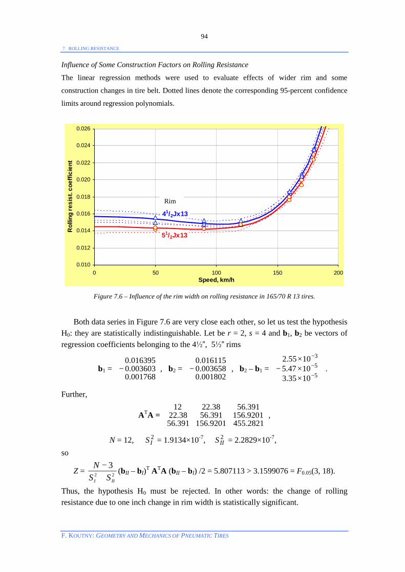
7 ROLLING RESISTANCE
F. KOUTNY: GEOMETRY AND MECHANICS OF PNEUMATIC TIRES
94
Influence of Some Construction Factors on Rolling Resistance
The linear regression methods were used to evaluate effects of wider rim and some
construction changes in tire belt. Dotted lines denote the corresponding 95-percent confidence
limits around regression polynomials.
0.010
0.012
0.014
0.016
0.018
0.020
0.022
0.024
0.026
0 50 100 150 200Speed, km/h
Rol
ling
resi
st. c
oeffi
cien
t
41/2Jx13
51/2Jx13
Figure 7.6 – Influence of the rim width on rolling resistance in 165/70 R 13 tires.
Both data series in Figure 7.6 are very close each other, so let us test the hypothesis H0: they are statistically indistinguishable. Let be r = 2, s = 4 and b1, b2 be vectors of regression coefficients belonging to the 4½”, 5½” rims
b1 =
−
001768.0003603.0016395.0
, b2 =
−
001802.0003658.0016115.0
, b2 – b1 =
××−×
−
−
−
553
1035.31047.51055.2
.
Further,
ATA =
2821.4559201.156391.569201.156391.5638.22391.5638.2212
,
N = 12, 2IS = 1.9134×10⁻⁷, 2
IIS = 2.2829×10⁻⁷, so
Z = N
S SI II
−+
32 2 (bII – bI)T ATA (bII – bI) /2 = 5.807113 > 3.1599076 = F0.05(3, 18).
Thus, the hypothesis H0 must be rejected. In other words: the change of rolling resistance due to one inch change in rim width is statistically significant.
Rim
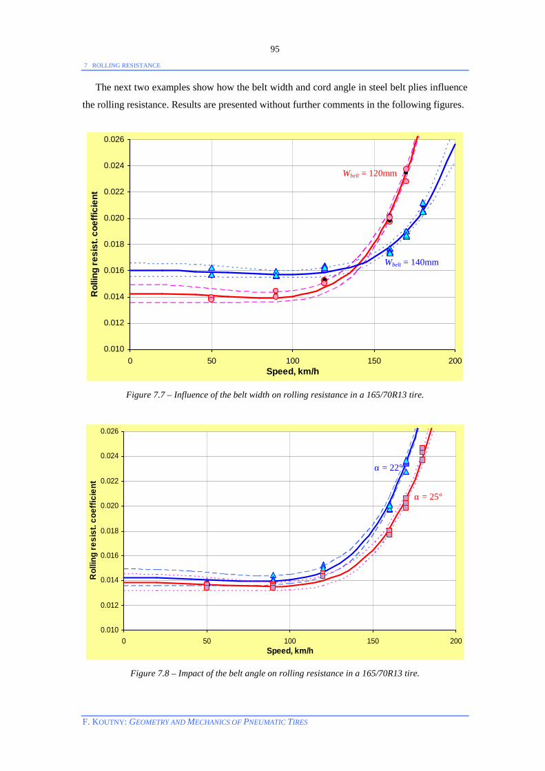
7 ROLLING RESISTANCE
F. KOUTNY: GEOMETRY AND MECHANICS OF PNEUMATIC TIRES
95
The next two examples show how the belt width and cord angle in steel belt plies influence
the rolling resistance. Results are presented without further comments in the following figures.
0.010
0.012
0.014
0.016
0.018
0.020
0.022
0.024
0.026
0 50 100 150 200Speed, km/h
Rol
ling
resi
st. c
oeffi
cien
t
Figure 7.7 – Influence of the belt width on rolling resistance in a 165/70R13 tire.
0.010
0.012
0.014
0.016
0.018
0.020
0.022
0.024
0.026
0 50 100 150 200Speed, km/h
Rol
ling
resi
st. c
oeffi
cien
t
Figure 7.8 – Impact of the belt angle on rolling resistance in a 165/70R13 tire.
α = 22°
α = 25°
Wbelt = 120mm
Wbelt = 140mm

7 ROLLING RESISTANCE
F. KOUTNY: GEOMETRY AND MECHANICS OF PNEUMATIC TIRES
96
7.3 Dependence of µ on Inflation Pressure and Load Tire rolling resistance plays a very important role in highway traffic. Tires in daily use do not run always in optimal conditions. Although their speed is bounded from above by legal limits they may be overloaded e.g. by low inflation pressure or high load. Then the question arises how the load and inflation pressure influence the rolling resistance at a given speed. As well known, rolling resistance depends substantially on two factors connected with tread/belt block: radial deflection u and contact pressure pmc, i.e.
R(p, FR) ≈ a0 + a1 u + a2 pmc. The following Figures 7.9, 7.10 show these quantities as functions of the inflation pressure p and vertical load FR in 295/80R22.5 tire on the road wheel with diameter 2m computed by means of belt model. The functions u(p, FR), pmc(p, FR) appear quite simple and smooth. The variables p, FR may be chosen independently in a convenient range. Then the coefficient of rolling resistance may be approximately represented by the following function
1000 µ(p, FR) ≈ β0 + β1 FR + β2 p1
.
In order to find the estimates b0, b1, b2 of coefficients β0, β1, β2 in 295/80R22.5 tires a statistically designed experiment was carried out [51,55].
500600
700800
90015
20
2530
350
10
20
30
40
50
60
70
Rad. deflection u , mm
Infl. pressure p , kPa
Vert. load F R , kN
60-70
50-6040-50
30-40
20-30
10-20
0-10
Figure 7.9 – Radial deflection u of the 295/80R22.5 tire on 2m-drum computed by belt model.
An acceptable and sufficiently large area for load FR and inflation pressure p at constant speed 70km/h was determined by the belt model so that tire destruction during testing was avoided. The radial deflection was limited by 50mm and the maximum
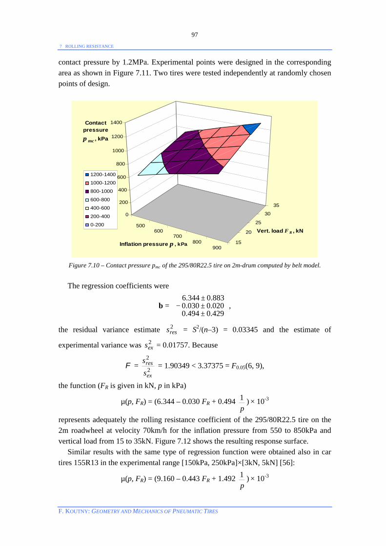
7 ROLLING RESISTANCE
F. KOUTNY: GEOMETRY AND MECHANICS OF PNEUMATIC TIRES
97
contact pressure by 1.2MPa. Experimental points were designed in the corresponding area as shown in Figure 7.11. Two tires were tested independently at randomly chosen points of design.
500600
700800
90015
20
25
30
35
0
200
400
600
800
1000
1200
1400Contact pressurep mc , kPa
Inflation pressure p , kPa
Vert. load F R , kN
1200-1400
1000-1200
800-1000
600-800
400-600
200-400
0-200
Figure 7.10 – Contact pressure pmc of the 295/80R22.5 tire on 2m-drum computed by belt model.
The regression coefficients were
β =
±±−±
429.0494.0020.0030.0883.0344.6
,
the residual variance estimate 2ress = S2/(n–3) = 0.03345 and the estimate of
experimental variance was 2exs = 0.01757. Because
F = 2
2
ex
res
ss
= 1.90349 < 3.37375 = F0.05(6, 9),
the function (FR is given in kN, p in kPa)
µ(p, FR) = (6.344 – 0.030 FR + 0.494 p1 ) × 10-3
represents adequately the rolling resistance coefficient of the 295/80R22.5 tire on the 2m roadwheel at velocity 70km/h for the inflation pressure from 550 to 850kPa and vertical load from 15 to 35kN. Figure 7.12 shows the resulting response surface. Similar results with the same type of regression function were obtained also in car tires 155R13 in the experimental range [150kPa, 250kPa]×[3kN, 5kN] [56]:
µ(p, FR) = (9.160 – 0.443 FR + 1.492 p1 ) × 10-3
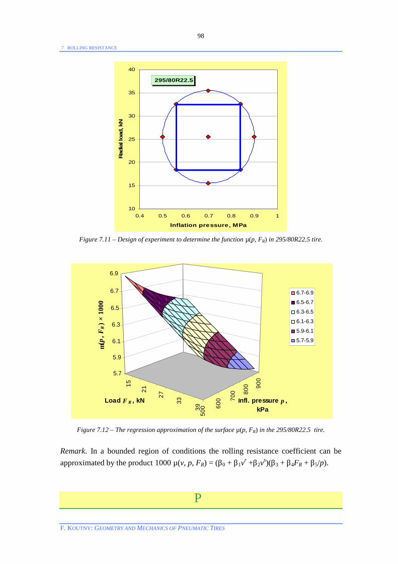
7 ROLLING RESISTANCE
F. KOUTNY: GEOMETRY AND MECHANICS OF PNEUMATIC TIRES
98
Figure 7.11 – Design of experiment to determine the function µ(p, FR) in 295/80R22.5 tire.
15
21
27
33
3950
0 600 70
0 800 90
0
5.7
5.9
6.1
6.3
6.5
6.7
6.9
µ(p
, FR
) × 1
000
Load F R , kN Infl. pressure p , kPa
6.7-6.9
6.5-6.7
6.3-6.5
6.1-6.3
5.9-6.1
5.7-5.9
Figure 7.12 – The regression approximation of the surface µ(p, FR) in the 295/80R22.5 tire.
Remark. In a bounded region of conditions the rolling resistance coefficient can be approximated by the product 1000 µ(v, p, FR) = (β0 + β1vr +β2vs)(β3 + β4FR + β5/p).
P
295/80R22.5
10
15
20
25
30
35
40
0.4 0.5 0.6 0.7 0.8 0.9 1
Inflation pressure, MPa
Rad
ial l
oad,
kN
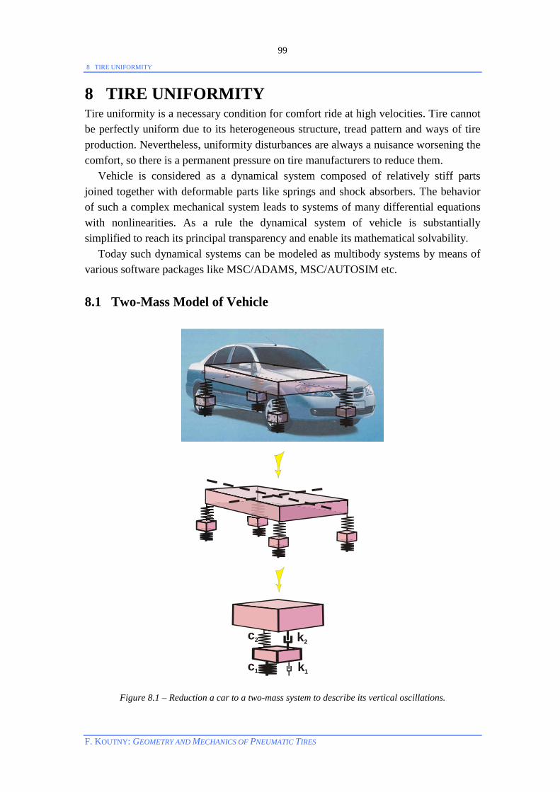
8 TIRE UNIFORMITY
F. KOUTNY: GEOMETRY AND MECHANICS OF PNEUMATIC TIRES
99
8 TIRE UNIFORMITY Tire uniformity is a necessary condition for comfort ride at high velocities. Tire cannot be perfectly uniform due to its heterogeneous structure, tread pattern and ways of tire production. Nevertheless, uniformity disturbances are always a nuisance worsening the comfort, so there is a permanent pressure on tire manufacturers to reduce them. Vehicle is considered as a dynamical system composed of relatively stiff parts joined together with deformable parts like springs and shock absorbers. The behavior of such a complex mechanical system leads to systems of many differential equations with nonlinearities. As a rule the dynamical system of vehicle is substantially simplified to reach its principal transparency and enable its mathematical solvability. Today such dynamical systems can be modeled as multibody systems by means of various software packages like MSC/ADAMS, MSC/AUTOSIM etc. 8.1 Two-Mass Model of Vehicle
c2 k2
c1 k1
Figure 8.1 – Reduction a car to a two-mass system to describe its vertical oscillations.
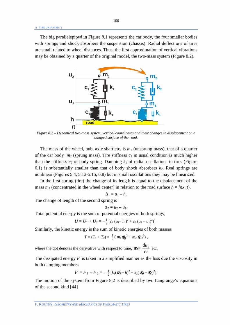
8 TIRE UNIFORMITY
F. KOUTNY: GEOMETRY AND MECHANICS OF PNEUMATIC TIRES
100
The big parallelepiped in Figure 8.1 represents the car body, the four smaller bodies with springs and shock absorbers the suspension (chassis). Radial deflections of tires are small related to wheel distances. Thus, the first approximation of vertical vibrations may be obtained by a quarter of the original model, the two-mass system (Figure 8.2).
c2 k2
c1 k1
m1
m2
0
u1
u2
c2 k2
c1 k1
m1
m2
h
Figure 8.2 – Dynamical two-mass system, vertical coordinates and their changes in displacement on a bumped surface of the road.
The mass of the wheel, hub, axle shaft etc. is m1 (unsprung mass), that of a quarter of the car body m2 (sprung mass). Tire stiffness c1 in usual condition is much higher than the stiffness c2 of body spring. Damping k1 of radial oscillations in tires (Figure 6.1) is substantially smaller than that of body shock absorbers k2. Real springs are nonlinear (Figures 5.4, 5.13-5.15, 6.8) but in small oscillations they may be linearized. In the first spring (tire) the change of its length is equal to the displacement of the mass m1 (concentrated in the wheel center) in relation to the road surface h = h(x, t),
∆1 = u1 – h. The change of length of the second spring is
∆2 = u2 – u1. Total potential energy is the sum of potential energies of both springs,
U = U1 + U2 = – 21 [c1 (u1– h )2 + c2 (u2 – u1)2)] .
Similarly, the kinetic energy is the sum of kinetic energies of both masses
T = (T1 + T2) = 21 ( m1 1u& 2 + m2 u& 2
2) ,
where the dot denotes the derivative with respect to time, 1u& = t
ud
d 1 etc.
The dissipated energy Φ is taken in a simplified manner as the loss due the viscosity in both damping members
Φ = Φ1 + Φ2 = – 21 [k1( 1u& – h)2 + k2( 2u& – 1u& )2].
The motion of the system from Figure 8.2 is described by two Langrange’s equations of the second kind [44]
road
8 TIRE UNIFORMITY
F. KOUTNY: GEOMETRY AND MECHANICS OF PNEUMATIC TIRES
101
−
∂∂ )(
dd UT
ut k& – )( UT
uk−
∂∂
= Φku&∂
∂ + Fk , k = 1, 2,
where Fk are external forces. Substituting T, U, Φ by corresponding expressions yields m1 1u&& + c1(u1 – h) – c2 (u2 – u1) = – k1(u& 1 – h& ) + k2 (u& 2 – u& 1) + F1,
m2 2u&& + c2(u2 – u1) = – k2 (u& 2 – u& 1) + F2 . When initial conditions are given this system of equations can be solved e.g. numerically [10]. But concrete solutions in time do not supply general view on the system behavior. Transfer functions or, more precisely, frequency characteristics are much more eloquent. The Laplace transform [9] gives for F1=F2=0 [51,57]
U 1(p) = 22222
222121
21
11222
2
][])][()([))((
cpkcpkpmccpkkpmpkccpkpm
+−+++++++++
H (p),
U 2(p) = 22222
222121
21
2211
][])][()([))((
cpkcpkpmccpkkpmcpkpkc
+−++++++++
H (p) ,
where H (p), U 1(p), U 2(p) are Laplace’s images of h(t), u1(t), u2(t). Putting p = iω gives formally Fourier’s images (i = 1− ). Let the denominator be written as the sum of real and imaginary parts,
D(iω) = R(ω) + i I(ω), where
R(ω) = Re D(iω) = m1m2 ω4 – [m1c2+(c1+c2)m2+k1k2] ω2 + c1c2 , I(ω) = Im D(iω) = (k1c1+c1k2) ω – [m2k1+(m1+m2)k2] ω3 .
Then the amplitude-frequency characteristics of the car body is
A(ω) = )(
))(( 2211
ω
ω+ω+
iii
Dkckc
= )()(
)()(22
21221
2222121
ω+ω
+ω+ω−
IR
kckckkcc .
The discomfort of the ride on the road surface is physiologically perceived through
the body acceleration. Integral transforms of car body acceleration 22 )(t
tud
d2 are simply
p2U 2(p), ω2A(ω), respectively. Example. Let us consider the following parameters:
c1 = 250 000 N/m (radial stiffness of tire), c2 = 30 000 N/m (stiffness of body springs), k1 = 3 kg/s (damping coefficient of tire), k2 = 2 000 kg/s (damping coefficient of body shock absorber), m1 = 50 kg (wheel + hub + axle), m2 = 400 kg (a quarter of sprung mass, i.e. body + passengers + load) .
Figure 8.3 shows the amplitude-frequency characteristics of the sprung mass for different radial stiffness of tire as practically proportional to the inflation pressure.

8 TIRE UNIFORMITY
F. KOUTNY: GEOMETRY AND MECHANICS OF PNEUMATIC TIRES
102
0
100
200
300
400
500
600
700
0 2 4 6 8 10 12 14 16 18 20
Frequency, Hz
Bod
y ac
cele
ratio
n/R
oad
disp
lace
men
t
Figure 8.3 – Amplitude-frequency characteristics of sprung mass acceleration for variable radial
stiffness of tire. Because real dynamic systems of automobiles are nonlinear in the first place and incomparably complex in comparison to the two-mass model more realistic estimates of transfer functions are obtained by means of spectral densities S(ω) of accelerations measured in convenient places of the automobiles and the spectral density S0(ω) of road displacements,
)(ωA = )()(
0 ωω
SS .
But the corresponding measurements are complicated, very particular and expensive. On the other hand, the computer modeling offers much cheaper possibilities. Their results, however, must be verified by measurements at several pilot points at least. 8.2 Disturbances of Radial Uniformity Generally, tires transmit spatial forces and are required to have sufficient adhesion to the support in all weather conditions. Tread pattern enhances the adhesion but at the same time it is a source of uniformity disturbances and noise emissions of the tire. Slices of tread, sidewalls, carcass and belt plies in building process are another source of such disturbances [52]. Variability of steel cord circumferential density in radial carcass of truck tire and other irregularities were discussed in [58,59]. The mentioned irregularities cause variability of force on rolling tire which can be tracked in a relatively easy way on special testers of uniformity. The principle of measuring the radial force is shown in Figure 8.4.
c1 = 250kN/m
c1 = 150kN/m
c1 = 50kN/m
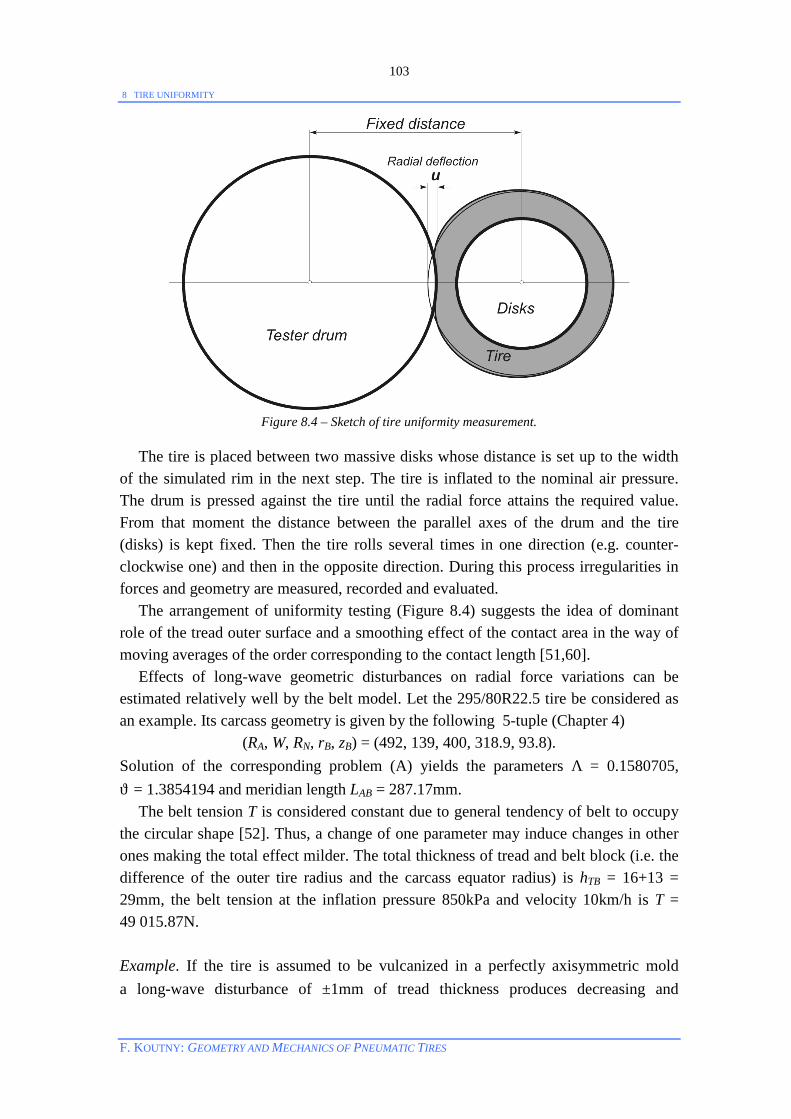
8 TIRE UNIFORMITY
F. KOUTNY: GEOMETRY AND MECHANICS OF PNEUMATIC TIRES
103
Figure 8.4 – Sketch of tire uniformity measurement.
The tire is placed between two massive disks whose distance is set up to the width of the simulated rim in the next step. The tire is inflated to the nominal air pressure. The drum is pressed against the tire until the radial force attains the required value. From that moment the distance between the parallel axes of the drum and the tire (disks) is kept fixed. Then the tire rolls several times in one direction (e.g. counter-clockwise one) and then in the opposite direction. During this process irregularities in forces and geometry are measured, recorded and evaluated. The arrangement of uniformity testing (Figure 8.4) suggests the idea of dominant role of the tread outer surface and a smoothing effect of the contact area in the way of moving averages of the order corresponding to the contact length [51,60]. Effects of long-wave geometric disturbances on radial force variations can be estimated relatively well by the belt model. Let the 295/80R22.5 tire be considered as an example. Its carcass geometry is given by the following 5-tuple (Chapter 4)
(RA, W, RN, rB, zB) = (492, 139, 400, 318.9, 93.8). Solution of the corresponding problem (A) yields the parameters Λ = 0.1580705, ϑ = 1.3854194 and meridian length LAB = 287.17mm. The belt tension T is considered constant due to general tendency of belt to occupy the circular shape [52]. Thus, a change of one parameter may induce changes in other ones making the total effect milder. The total thickness of tread and belt block (i.e. the difference of the outer tire radius and the carcass equator radius) is hTB = 16+13 = 29mm, the belt tension at the inflation pressure 850kPa and velocity 10km/h is T = 49 015.87N. Example. If the tire is assumed to be vulcanized in a perfectly axisymmetric mold a long-wave disturbance of ±1mm of tread thickness produces decreasing and
8 TIRE UNIFORMITY
F. KOUTNY: GEOMETRY AND MECHANICS OF PNEUMATIC TIRES
104
increasing the carcass equator radius of 491 and 493mm, while the tire width as well as the beads remain unchanged. The changes of meridian length can be estimated in a simplified way by solving the following two problems (A)
((RA*, W, RN, rB, zB) → (Λ, ϑ),
where RA* = 491 and 493mm. One obtains
RA, mm Λ ϑ, rad. LAB, mm T, N 491 0.1573085 1.3839069 286.42 49 391.56 493 0.1588227 1.3869022 287.94 48 653.44
The constant belt tension may be supposed to be the original value T = 49 015.87N. Changes of T at different meridional lengths are eliminated by changing the carcass equator radius (found by interpolation):
hTB RA, mm 17 + 13 491.391 15 + 13 492.625
Hence, the carcass run-out caused by the 2mm-difference in tread thickness is ∆R = 1.234mm.
The belt model gives also radial load-deflection curves corresponding to different tread thicknesses:
hTB RA(hTB), mm F(u), N 30 491.391 –0.00940 u3 + 5.26867 u2 + 669.803 u 29 492.000 –0.00933 u3 + 5.25550 u2 + 670.142 u 28 492.625 –0.00925 u3 + 5.24225 u2 + 670.478 u
The perfect tire with the outer radius 492 + 29 = 521mm at 850kPa and radial deflection 37mm corresponding to radial load 31.5kN on uniformity tester drum with radius 800mm determines the distance between the axes of revolution of both tire and drum
d = 800 + 492 + 29 – 37 = 1284mm . Let this distance be fixed, d = 800 + R(hTB)A + hTB – u = 1284mm. Then the radial deflection of the tire in a place with another tread thickness hTB is
u(hTB) = – d + 800 + RA(hTB) + hTB = RA(hTB) + hTB – 484 . Now the corresponding radial loads, F(u(hTB)), can be computed from the formulas written above:
hTB, mm u(hTB), mm F(u), N 30 37.391 31 919.27 29 37.000 31 519.38 28 36.625 31 137.07
Thus, the rate caused by a long wave variability of the tread-belt thickness is

8 TIRE UNIFORMITY
F. KOUTNY: GEOMETRY AND MECHANICS OF PNEUMATIC TIRES
105
TB
TBhhF
dd )(
≈ 2
07.1373127.91931 − ≈ 391N/mm ,
the rate of tread radial run-out
TB
TBhhR
dd )(
= TB
TBTBh
hhRd
d( A ))( + ≈ 1 +
2492.625-491.391 ≈ 0.383
and the rate of carcass radial run-out
TB
TBh
hRd
d A )(≈
2625492391491 .. − ≈ – 0.617 .
The ideal relationship between radial force variation and tread or carcass run-out is
)()(
TB
TBhRhF
dd
≈ 383.0
391 ≈ 1020.9N/mm or )
)(
TBA
TBhR
hF(d
d ≈
617.0391 ≈ 633.7N/mm.
In a series of 4 273 of the 285/80R22.5 tires the average ratio QR of radial force variation and radial run-out was 605.2N/mm with the sample standard deviation 131.2N/mm, in another series of 4021 of those tires the average ratio of radial force variation and radial run-out was 628.5N/mm with the sample standard deviation 234.2N/mm. Hence, )/)( TBATB hRhF (dd appears to be a quite acceptable
approximation of QR. Impact of the sidewall or bead apex thickness variability, bead bundle eccentricity etc. on radial uniformity can be estimated in a similar way.
Any serious measurement must be repeatable. Repeatability was verified by detailed measurements along the circumference of the 295/80R22.5 tire carried out one after another four times [51,60]. In regular regime of measurement the following seven quantities are recorded in 128 equidistant positions φk = 2πk/128: k = 0, 1, …, 127 of the circumferential angle.
1. radial force deviation in the clockwise direction, 2. lateral force deviation in the clockwise direction, 3. radial force deviation in the counterclockwise direction, 4. lateral force deviation in the counterclockwise direction, 5. radial run out on the tire equator, 6. axial run out on the sidewall from the bottom part of the vulcanization mold, 7. axial run out on the sidewall from the upper part of the vulcanization mold.
Evident periodicity of forces and run outs leads to their decomposition in harmonic components. E.g. the radial force can be written as the following trigonometric polynomial in the phasor form [10]
Sn(φ) = r0 + ∑=
n
k 1rk sin(kφ + φk),
where rk = 22kk ba + is the amplitude and φk the phase of the kth harmonic,
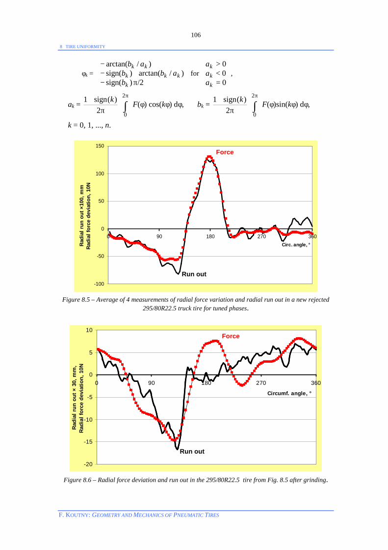
8 TIRE UNIFORMITY
F. KOUTNY: GEOMETRY AND MECHANICS OF PNEUMATIC TIRES
106
φk =
π−+−
−
/2)sign()arctan()sign(
)arctan(
kkkk
kk
babb
ab/
/ for
000
=<>
kkk
aaa
,
ak = π
+2
sign )(1 k ∫π2
0
F(φ) cos(kφ) dφ, bk = π
+2
sign )(1 k ∫π2
0
F(φ)sin(kφ) dφ,
k = 0, 1, ..., n.
-100
-50
0
50
100
150
0 90 180 270 360Circ. angle, °R
adia
l run
out
×10
0, m
m
Radi
al fo
rce
devi
atio
n, 1
0N
Figure 8.5 – Average of 4 measurements of radial force variation and radial run out in a new rejected
295/80R22.5 truck tire for tuned phases.
-20
-15
-10
-5
0
5
10
0 90 180 270 360
Circumf. angle, °
Rad
ial r
un o
ut ×
30,
mm
,R
adia
l for
ce d
evia
tion,
10N
Figure 8.6 – Radial force deviation and run out in the 295/80R22.5 tire from Fig. 8.5 after grinding.
Force
Run out
Force
Run out
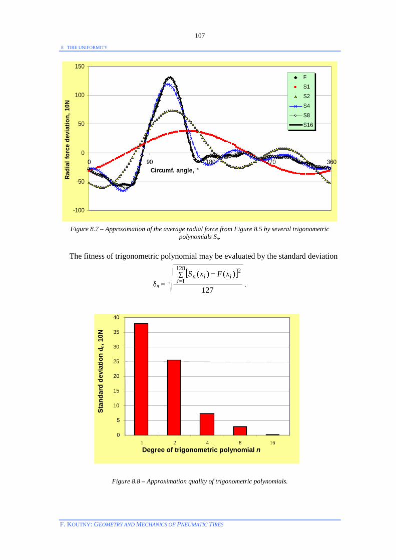
8 TIRE UNIFORMITY
F. KOUTNY: GEOMETRY AND MECHANICS OF PNEUMATIC TIRES
107
-100
-50
0
50
100
150
0 90 180 270 360Circumf. angle, °
Radi
al fo
rce
devi
atio
n, 1
0NFS1
S2
S4S8
S16
Figure 8.7 – Approximation of the average radial force from Figure 8.5 by several trigonometric
polynomials Sn. The fitness of trigonometric polynomial may be evaluated by the standard deviation
δn = [ ]
127
128
1
2∑=
−i
iin xFxS )()(.
Figure 8.8 – Approximation quality of trigonometric polynomials.
0
5
10
15
20
25
30
35
40
1 2 4 8 16 Degree of trigonometric polynomial n
Stan
dard
dev
iatio
n δ n
, 10N
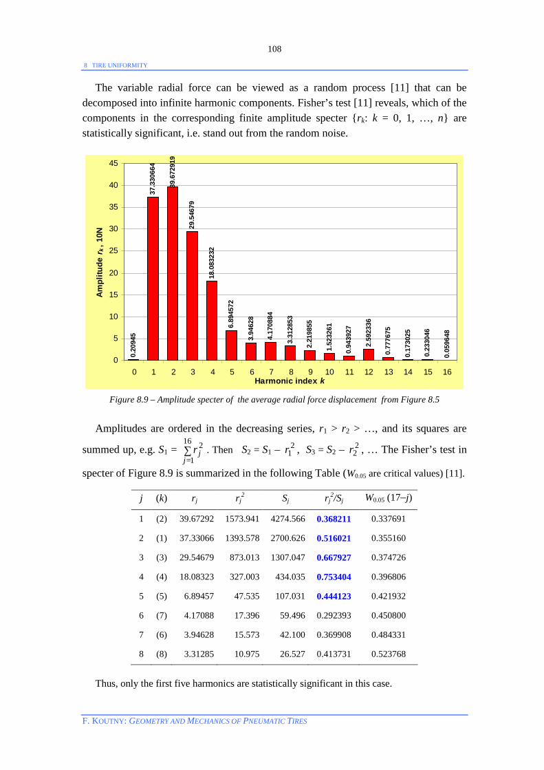
8 TIRE UNIFORMITY
F. KOUTNY: GEOMETRY AND MECHANICS OF PNEUMATIC TIRES
108
The variable radial force can be viewed as a random process [11] that can be decomposed into infinite harmonic components. Fisher’s test [11] reveals, which of the components in the corresponding finite amplitude specter rk: k = 0, 1, …, n are statistically significant, i.e. stand out from the random noise.
0.20
945
37.3
3066
4
39.6
7291
9
29.5
4679
18.0
8323
2
6.89
4572
3.94
628
4.17
0884
3.31
2853
2.21
9855
1.52
3261
0.94
3927
2.59
2336
0.77
7675
0.17
3025
0.23
3046
0.05
9648
0
5
10
15
20
25
30
35
40
45
0 1 2 3 4 5 6 7 8 9 10 11 12 13 14 15 16Harmonic index k
Ampl
itude
rk, 1
0N
Figure 8.9 – Amplitude specter of the average radial force displacement from Figure 8.5
Amplitudes are ordered in the decreasing series, r1 > r2 > …, and its squares are
summed up, e.g. S1 = ∑=
16
1
2
jjr . Then S2 = S1 – 2
1r , S3 = S2 – 22r , … The Fisher’s test in
specter of Figure 8.9 is summarized in the following Table (W0.05 are critical values) [11].
j (k) rj rj2 Sj rj
2/Sj W0.05 (17–j)
1 (2) 39.67292 1573.941 4274.566 0.368211 0.337691
2 (1) 37.33066 1393.578 2700.626 0.516021 0.355160
3 (3) 29.54679 873.013 1307.047 0.667927 0.374726
4 (4) 18.08323 327.003 434.035 0.753404 0.396806
5 (5) 6.89457 47.535 107.031 0.444123 0.421932
6 (7) 4.17088 17.396 59.496 0.292393 0.450800
7 (6) 3.94628 15.573 42.100 0.369908 0.484331
8 (8) 3.31285 10.975 26.527 0.413731 0.523768
Thus, only the first five harmonics are statistically significant in this case.

8 TIRE UNIFORMITY
F. KOUTNY: GEOMETRY AND MECHANICS OF PNEUMATIC TIRES
109
8.3 Distribution of Low-Speed Uniformity Disturbances Standard tire uniformity measurements are carried out at very low speeds of 1 revolution/s, i.e. less than 10km/h in car tires. The measurement result is a vector
x =
mx
xM1
,
whose components are: x1 = RFV (Radial Force Variation peak to peak), x2 = r1 = H1 (Amplitude of the first harmonic in radial force), x3 = LFV (Lateral Force Variation peak to peak), x4 = CON (Conicity), x5 = TRO (Top Run Out of the upper sidewall (in mold)), x6 = BRO (Bottom Run Out of the lower sidewall (in mold)), x7 = RRO (Radial Run Out on equator).
This list may be extended by further items, e.g. ply steer PS, further harmonics in radial (H2, …) and lateral (LH1, LH2, …) forces, run out in different positions on tread or sidewall etc. The rolling direction may be respected as well. Components x1, …, xm are random variables bounded from above and from below, similarly like strength of materials [39]. For example, radial or lateral force disturbances cannot be negative and cannot be greater than e.g. nominal load of tire. This is valid also for conicity although it may be of both signs, positive or negative. Thus, a component of uniformity disturbance is a random variable from some final interval I = [b1, b2]. As a rule, its relative frequency (probability density) f increases from f(b1) = 0 to a maximum f(xmax) > 0 (modus), b1 < xmax < b2, and then decreases to f(b2) = 0. The following product is one of such simple and smooth functions
A ( ) ( )3 4
1 2b bx b b x− − , A, b3, b4 > 0.
This function defines a probability density only if it is normed, i.e.
A ∫2
1
b
b( ) ( )3 4
1 2b bx b b x− − dx = 1 .
The function
t(x) = 1
2 1
x bb b
−−
is one-to-one mapping [b1, b2] → [0, 1] . Hence
∫2
1
b
b( ) ( )3 4
1 2b bx b b x− − dx = ( ) 3 4 1
2 1b bb b + +−
1
0∫ 3 4(1 ) db bt t t− = ( ) 3 4 1
2 1b bb b + +− B(b3+1, b4+1) ,
where B is the well known Euler’s Beta function [39]. Between this and more frequently used Gamma function [9, 39] is the following connection

8 TIRE UNIFORMITY
F. KOUTNY: GEOMETRY AND MECHANICS OF PNEUMATIC TIRES
110
B(b3+1, b4+1) = )2(
)1()1(
43
43++Γ
+Γ+Γbb
bb.
The corresponding (cumulative) distribution function is then
F(x, b) = )1()1(
)2(
43
43+Γ+Γ
++Γbb
bb∫−−
12
1
0
bbbx
3 4(1 ) db bt t t− ,
where b = (b1, …, b4)T is the unknown vector of parameters. It may be defined by minimization of the function
X2(b) = i
iiK
i npnpn 2
1
)( −∑=
.
Here n is the total number of elements in the considered series of tires. The interval of measurement I = [b1, b2] is decomposed into K subintervals Ii (classes), ni are frequencies (numbers of elements in Ii) and npi are ´theoretical´ frequencies,
pi = ∫iI
d F(x, b) .
Parameters b1, …, b4 are found by direct minimization of X2(b) based on genetic algorithm [10,39]. For great n the quantity X2(b) belongs to χ2(K–1) distribution. This enables testing the goodness of fit [11,54] by comparing X2(b) to the critical value χ2
α(K–1– 4). In other words, the fraction X2(b)/ χ2
α(K–1– 4) must be < 1. Example. A series of the 385/55R22.5 tires of range n = 786 was decomposed into K = 16 classes with respect to lateral force variation (LFV). The search for minimum of X2(b) gave the following results (∆α denotes confidence limit for probability level α
under the assumption of normality of bk, ∆α = u1–α/2 s / r , where u1–α/2 is the quantile of N(0, 1), s is standard deviation and r = 5 is number of calculation repetitions)
Run 1 Run 2 Run 3 Run 4 Run 5 ∆0.05
b1 1.494 2.016 1.822 1.771 1.358 0.061
b2 35.435 32.580 34.996 35.672 35.664 1.502
b3 5.533 4.581 4.999 5.121 5.759 0.187
b4 19.180 15.358 17.967 18.748 19.718 2.564
X2 2.086 2.499 2.125 2.046 2.164
X2/χ20.05 0.106 0.127 0.108 0.104 0.110
The minimum X2(b) was obtained in the 4th run (shadowed column) and is taken as the parameter vector estimate b. Thus,
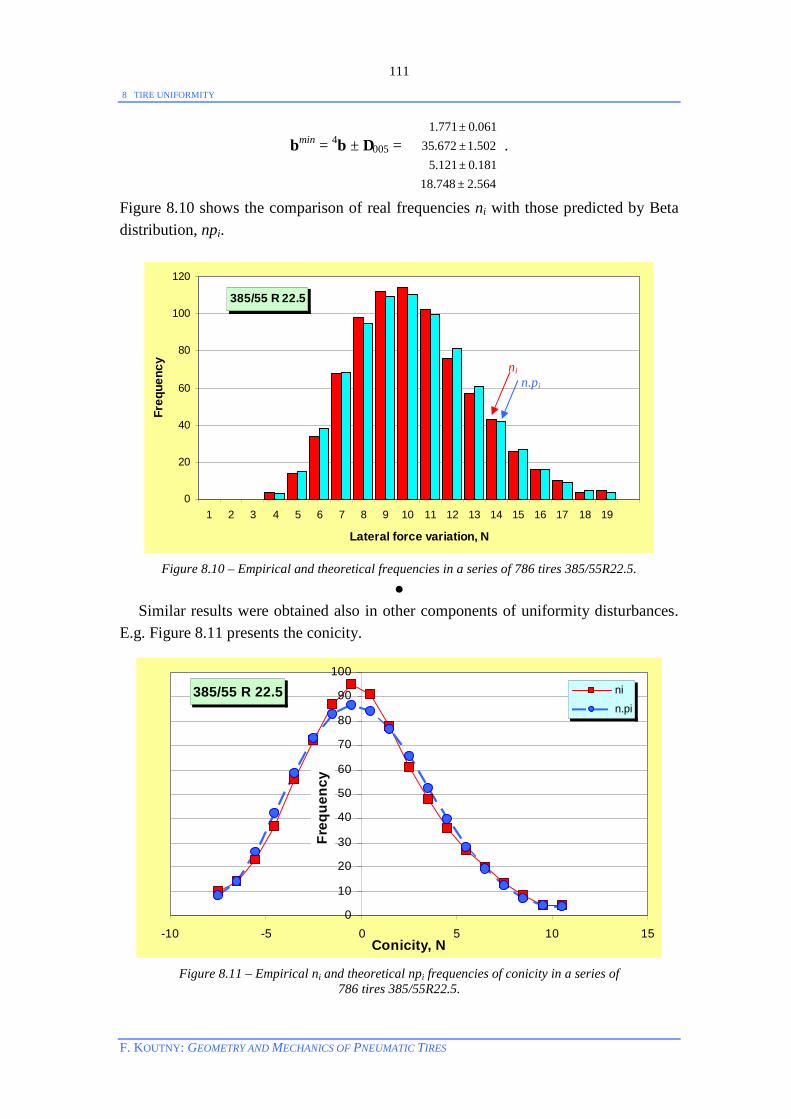
8 TIRE UNIFORMITY
F. KOUTNY: GEOMETRY AND MECHANICS OF PNEUMATIC TIRES
111
bmin = 4b ± ∆005 = 1.771 0.06135.672 1.502
5.121 0.181 18.748 2.564
± ± ±
±
.
Figure 8.10 shows the comparison of real frequencies ni with those predicted by Beta distribution, npi.
385/55 R 22.5
0
20
40
60
80
100
120
1 2 3 4 5 6 7 8 9 10 11 12 13 14 15 16 17 18 19
Lateral force variation, N
Freq
uenc
y
Figure 8.10 – Empirical and theoretical frequencies in a series of 786 tires 385/55R22.5.
Similar results were obtained also in other components of uniformity disturbances. E.g. Figure 8.11 presents the conicity.
385/55 R 22.5
0
10
20
30
40
50
60
70
80
90
100
-10 -5 0 5 10 15Conicity, N
Freq
uenc
y
ni
n.pi
Figure 8.11 – Empirical ni and theoretical npi frequencies of conicity in a series of
786 tires 385/55R22.5.
ni n.pi

8 TIRE UNIFORMITY
F. KOUTNY: GEOMETRY AND MECHANICS OF PNEUMATIC TIRES
112
The choice of probability distribution is free. Other distributions are suggested in [39], e.g. the double–branch normal distribution DN(b1, b2, b3). Its density,
fDN(x; b1, b2, b3) =
>
−−
+π
≤
−−
+π
1
2
3
1
32
1
2
2
1
32
2exp/2
2exp/2
bxb
bxbb
bxb
bxbb
for ,
is positive in the whole real axis R1. This, of course, contradicts the requirement of boundedness of measured quantities. The same fault appears in correspondingly generalized Weibull distribution that could be considered for some positive quantities. The following Table presents ratios X2(b)/ χ2
α(K–1–p) for different probability distributions (p = 2 in normal distribution, p = 3 in D-normal distribution and p = 4 in beta
distribution) and speaks in favor of beta distribution.
Tire size n X Normal d. D-normal d. Beta distr. 385/55 R 22.5 786 RFV 1.020 0.202 0.204
H1 0.924 0.379 0.378 LFV 1.552 0.140 0.104 CON 0.539 0.128 0.193 PS 0.410 0.529 0.354 TRO 0.940 0.143 0.103 BRO 2.335 0.058 0.183 RRO 0.781 0.068 0.065 385/65 R 22.5 1 842 RFV 3.880 0.821 0.721 H1 2.568 0.400 0.397 LFV 3.011 0.532 0.373 315/80 R 22.5 4 517 RFV 3.753 0.860 0.438 H1 6.630 0.486 0.247 LFV 6.500 0.545 0.472 295/80 R 22.5 4 273 RFV 5.541 0.560 0.703 H1 7.078 0.580 0.815 LFV 10.907 0.931 0.738 CON 7.218 0.975 0.449 TRO 8.048 0.864 0.541 BRO 4.302 0.754 0.281 RRO 7.605 0.846 0.695 295/80 R 22.5 4 022 RFV 2.383 0.238 0.252 H1 2.825 0.985 0.718 LFV 8924 0.513 0.732 RRO 6.384 0.515 0.770 275/70 R 22.5 1 178 RFV 2.091 0.328 0.284 H1 2.275 0.921 0.370 LFV 3.023 0.229 0.211 CON 0.326 0.509 0.578 TRO 2.137 0.251 0.348 BRO 3.501 0.351 0.524 RRO 2.200 0.261 0.338
Sum of testing ratios 121.611 15.902 13.579

8 TIRE UNIFORMITY
F. KOUTNY: GEOMETRY AND MECHANICS OF PNEUMATIC TIRES
113
8.4 Correlation among Uniformity Components Individual quantities registered in tire uniformity testing may appear independent or joined mutually. The correlation coefficient shows a quantitative evaluation of the dependence degree between two simple quantities. In vector quantities it is substituted by correlation matrix whose entries are the customary correlation coefficients [11]. Results of uniformity testing in a series of tires can be written as an n×m matrix, where n is the number of tires in the series and m is the number of measured quantities,
X =
−−−
mnnn
mnnn
mm
xxxxxx
xxxxxx
,2,1,
,12,11,1
2222111211
...
...............
...
...
= (x1, …, xm) .
Columns x1, …, xm represent the measured quantities. The sample correlation coefficient of vectors xj, xk is the number
rjk = ∑∑
∑
==
=
−−
−−
n
ikji
n
ijji
n
ikjijji
xxxx
xxxx
1
2
1
2
1
)()(
))((,
where jx = ∑=
n
ijix
n 1
1, kx = ∑
=
n
ikix
n 1
1 are the column averages. The numbers rjk are entries
of the m×m symmetric matrix R. Obviously, rjj = 1, j = 1, …, m. Critical value of the correlation coefficient for the n-dimensional vectors (n>2) and the significance level α is [11,54]
rα(n) = 21
2 )2(21
−
α
−
−+
ntn ,
where tα(n–2) is the corresponding critical value of t-distribution. Here is an example of the correlation matrix in a series of tires 385/55R22.5 in which eight components of uniformity were registered (n = 786, r0.05(784) = 0.06994). Entries above the diagonal need to be written only, due to symmetry.
H1 LFV CON PS TRO BRO RRO
RFV 0.9037 0.0220 0.0577 -0.0108 -0.0183 0.0301 0.8397
H1 -0.0048 0.0866 0.0002 -0.0015 0.0166 0.7687
LFV 0.0136 0.0556 -0.0201 -0.0506 0.0528
CON -0.1316 0.0196 0.0722 0.0699
PS -0.0639 -0.0238 -0.0020
TRO 0.1926 -0.0309
BRO 0.0048
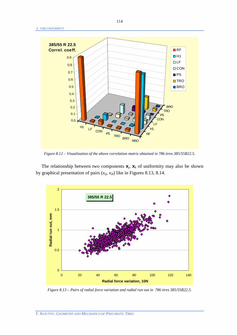
8 TIRE UNIFORMITY
F. KOUTNY: GEOMETRY AND MECHANICS OF PNEUMATIC TIRES
114
H1 LF CONPS
TROBRO
RRO
RFH1
LFCON
PSTRO
BRO
0.0
0.1
0.2
0.3
0.4
0.5
0.6
0.7
0.8
0.9
385/55 R 22.5Correl. coeff. RF
H1
LF
CON
PS
TRO
BRO
Figure 8.12 – Visualization of the above correlation matrix obtained in 786 tires 385/55R22.5.
The relationship between two components xj, xk of uniformity may also be shown by graphical presentation of pairs (xij, xik) like in Figures 8.13, 8.14.
385/55 R 22.5
0
0.5
1
1.5
2
0 20 40 60 80 100 120 140
Radial force variation, 10N
Rad
ial r
un o
ut, m
m
Figure 8.13 – Pairs of radial force variation and radial run out in 786 tires 385/55R22.5.
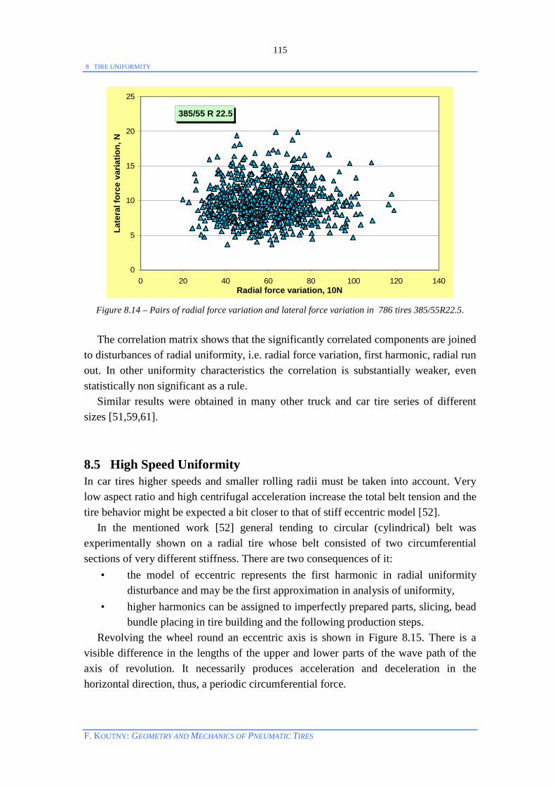
8 TIRE UNIFORMITY
F. KOUTNY: GEOMETRY AND MECHANICS OF PNEUMATIC TIRES
115
385/55 R 22.5
0
5
10
15
20
25
0 20 40 60 80 100 120 140Radial force variation, 10N
Late
ral f
orce
var
iatio
n, N
Figure 8.14 – Pairs of radial force variation and lateral force variation in 786 tires 385/55R22.5.
The correlation matrix shows that the significantly correlated components are joined to disturbances of radial uniformity, i.e. radial force variation, first harmonic, radial run out. In other uniformity characteristics the correlation is substantially weaker, even statistically non significant as a rule. Similar results were obtained in many other truck and car tire series of different sizes [51,59,61]. 8.5 High Speed Uniformity In car tires higher speeds and smaller rolling radii must be taken into account. Very low aspect ratio and high centrifugal acceleration increase the total belt tension and the tire behavior might be expected a bit closer to that of stiff eccentric model [52]. In the mentioned work [52] general tending to circular (cylindrical) belt was experimentally shown on a radial tire whose belt consisted of two circumferential sections of very different stiffness. There are two consequences of it:
• the model of eccentric represents the first harmonic in radial uniformity disturbance and may be the first approximation in analysis of uniformity,
• higher harmonics can be assigned to imperfectly prepared parts, slicing, bead bundle placing in tire building and the following production steps.
Revolving the wheel round an eccentric axis is shown in Figure 8.15. There is a visible difference in the lengths of the upper and lower parts of the wave path of the axis of revolution. It necessarily produces acceleration and deceleration in the horizontal direction, thus, a periodic circumferential force.
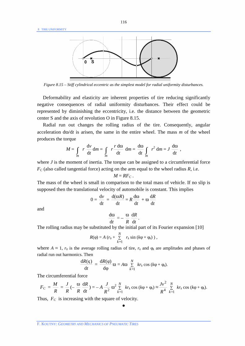
8 TIRE UNIFORMITY
F. KOUTNY: GEOMETRY AND MECHANICS OF PNEUMATIC TIRES
116
Figure 8.15 – Stiff cylindrical eccentric as the simplest model for radial uniformity disturbances.
Deformability and elasticity are inherent properties of tire reducing significantly negative consequences of radial uniformity disturbances. Their effect could be represented by diminishing the eccentricity, i.e. the distance between the geometric center S and the axis of revolution O in Figure 8.15. Radial run out changes the rolling radius of the tire. Consequently, angular acceleration dω/dt is arisen, the same in the entire wheel. The mass m of the wheel produces the torque
M = ∫m
r tv
dd dm = ∫
m
rt
rdd ω dm =
tddω
∫m
r2 dm = J td
dω ,
where J is the moment of inertia. The torque can be assigned to a circumferential force FC (also called tangential force) acting on the arm equal to the wheel radius R, i.e.
M = RFC . The mass of the wheel is small in comparison to the total mass of vehicle. If no slip is supposed then the translational velocity of automobile is constant. This implies
0 = tv
dd =
tR
dd( )ω = R
tddω + ω
tR
dd
and
tddω = –
Rω
tR
dd .
The rolling radius may be substituted by the initial part of its Fourier expansion [10]
R(φ) = A (r0 + ∑=
N
k 1 rk sin (kφ + φk) ) ,
where A ≈ 1, r0 is the average rolling radius of tire, rk and φk are amplitudes and phases of radial run out harmonics. Then
tRd
d )(φ = φφ
dd )(R
ω = Aω ∑=
N
k 1krk cos (kφ + φk).
The circumferential force
FC = RM =
RJ (–
Rω
tR
dd ) = – A 2R
Jω2 ∑
=
N
k 1krk cos (kφ + φk) ≈ 4
2
RJv
∑=
N
k 1krk cos (kφ + φk).
Thus, FC is increasing with the square of velocity.

8 TIRE UNIFORMITY
F. KOUTNY: GEOMETRY AND MECHANICS OF PNEUMATIC TIRES
117
To illustrate the high speed uniformity two series of tires were chosen: • 235/40R18 tires, n = 518 and • 235/60R18 tires, n = 1 216. Main parameters of those tires are as follows: Tire 235/40R18 235/60R18 Overall diameter, mm 645 739 Overall width, mm 241 240 Rim 8.5×18 7.5×18 Belt model parameters: Carcass equator radius RA, mm 309.5 356.5 A half of carcass ´width´ W, mm 115.5 115.0 Carcass curvature radius in belt area RAN, mm 3000.0 1000.0 Bead point radial coordinate rB, mm 249.8 250.3 Bead point axial coordinate zB, mm 104.4 92.3
Figure 8.16 – Sketches of belt models for the 235/40R18 and 235/60R18 tires. Distribution of low speed radial force variation is presented in Figure 8.17. Squares represent real frequencies ni in total n tires, while continuous lines and small circles belong to Beta distribution and theoretical frequencies npi.

8 TIRE UNIFORMITY
F. KOUTNY: GEOMETRY AND MECHANICS OF PNEUMATIC TIRES
118
0
0.05
0.1
0.15
0.2
0.25
0.3
0.35
0 2 4 6 8 10 12 14Radial force variation, 10N
(Rel
. fre
q.)/(
Cla
ss w
idth
)
Figure 8.17 – Distribution of radial force variation in two series of car tires at low speed (v = 8km/h). The distribution of uniformity disturbances is changed dramatically at high speeds. This is illustrated in the following two figures.
235/60R18
0
0.05
0.1
0.15
0.2
0.25
0 5 10 15 20 25 30Radial force variation, 10N
(Rel
. fre
q.)/(
Cla
ss w
idth
)
Figure 8.18 – Distribution of radial force variation in 235/60R18 tires at speeds 8km/h and 120km/h.
235/40R18
235/60R18
v = 120km/h
v = 8km/h

8 TIRE UNIFORMITY
F. KOUTNY: GEOMETRY AND MECHANICS OF PNEUMATIC TIRES
119
235/40R18
0
0.02
0.04
0.06
0.08
0.1
0.12
0.14
0.16
0.18
0 5 10 15 20 25 30Radial force variation, 10N
Rel
ativ
e fr
eque
ncy
Figure 8.19 – Distribution of radial force variation in 235/40R18 tires at speeds 8km/h and 120km/h.
The influence of the changes of velocity on lateral force variability is shown in Figure 8.20.
235/40R18
0
0.02
0.04
0.06
0.08
0.1
0.12
0.14
0.16
0.18
0 2 4 6 8 10 12Lateral force variation, 10N
Rel
ativ
e fr
eque
ncy
Figure 8.20 – Distribution of lateral force variation in 235/40R18 tires at speeds 8km/h and 120km/h.
It can be said generally that the correlations among different uniformity parameters (components) illustrated in Section 8.3 on several samples of truck tires preserve its validity also in car tires. But high speeds give rise to the question concerning the relation between low speed parameters and high speed parameters. If the real tires behaved like a stiff eccentric there would be a very strong correlation between uniformity parameters at velocities v = 8km/h and v = 120km/h. The following figure shows, however, that the connection between radial force variations at low and high speeds can be unexpectedly weak.
v = 8km/h v = 120km/h
v = 8km/h v = 120km/h

8 TIRE UNIFORMITY
F. KOUTNY: GEOMETRY AND MECHANICS OF PNEUMATIC TIRES
120
235/40R18
R2 = 0.2265
0
5
10
15
20
25
30
35
40
0 5 10 15 20 25Slow-speed radial force variation, 10N
High
-spe
ed ra
d. fo
rce
varia
tion,
10N
Figure 8.21 – Weak relationship between radial force variations at speeds of 8 and 120km/h.
This fact does not sound very encouragingly because tires perform regularly at high speeds while standard uniformity tests are performed at very low speeds. This way the value of standard low speed uniformity tests is reduced. It should also be taken into account that the shorter contact length on drum significantly diminishes the smoothing effect of contact area making the force uniformity tests more severe [51,60]. The model of stiff eccentric predicts a strong coupling of circumferential forces with radial run out at high speeds but this is not always true in real tires (Figure 8.22).
235/40R18, v = 120km/h
R2 = 0.0045
0
5
10
15
20
25
30
35
40
45
50
0 5 10 15 20 25 30 35 40Radial force variation, 10N
Circ
umf.
forc
e va
riatio
n, 1
0N
Figure 8.22 – Weak correlation between radial and circumferential force variations at 120km/h.

8 TIRE UNIFORMITY
F. KOUTNY: GEOMETRY AND MECHANICS OF PNEUMATIC TIRES
121
8.6 – Concluding remarks Tire testing could be viewed as a comprehensive autonomous science that uses special tools of mechanics and thermodynamics, electronics, informatics, statistics. The inherent variability of almost all parameters and characteristics of tire contribute significantly to the complexity of mathematical modeling of tire behavior. The following Figures 8.23 and 8.24 show examples of radial force and run out variance in a new tire and the same tire after its rolling on the roadwheel for several hours.
Tire 295/80R22.5 (1)
-40
-30
-20
-10
0
10
20
30
40
0 90 180 270 360
Circumf. angle, °
Rad
ial f
orce
var
iatio
n, 1
0 N
ClockwiseCounterclockwiseClockwiseCounterclockwise
Figure 8.23 – Change of radial force variation due to several hours of rolling the loaded tire on the
roadwheel.
Tire 295/80R22.5 (1)
-0.5
-0.4
-0.3
-0.2
-0.1
0.0
0.1
0.2
0.3
0.4
0.5
0 90 180 270 360
Circumf. angle, ° Rad
ial r
un o
ut, m
m
Figure 8.24 – Change of radial run out due to several hours of rolling the loaded tire on the roadwheel.
New Run
Run New

8 TIRE UNIFORMITY
F. KOUTNY: GEOMETRY AND MECHANICS OF PNEUMATIC TIRES
122
Similar variability can be found in high-speed uniformity. With another series of the 235/40R18 tires a high degree of correlation was obtained (Figure 8.25).
235/40R18 v = 120km/h
R2 = 0.713
0
20
40
60
0 10 20 30 40 50 60Radial force variation, 10N
Cir
cum
f. fo
rce
varia
tion,
10
N
Figure 8.25 – Correlation between radial and circumferential force variations at 120km/h in another
series of the 235/40R18 tires. Thus, results and conclusions obtained by processing measured data samples are always obtained only within some statistical confidence. Generally, the tire uniformity, especially the high speed uniformity, still remains an open and challenging theme.
P
9 COMPLEMENTARY THEMES
F. KOUTNY: GEOMETRY AND MECHANICS OF PNEUMATIC TIRES
123
9 SUPPLEMENTARY THEMES 9.1 Hydroplaning Hydroplaning is slipping the tire on the layer of water at high speeds similar to ice skating or skiing. In slips on the ice or snow a thin layer of water arises due to contact pressure and friction and the skate, ski, etc. moves almost without any resistance on that lubricating layer. A similar behavior can occur in tire on flooded road in torrential rain. The older literature says that critical speed, i.e. the speed at which the friction on the tire/road interface drops practically to zero, is proportional to the square root of the average contact pressure. This, however, is a too general conclusion. Recently many attempts were made to model the hydroplaning directly as a problem of hydrodynamics using modern numerical methods of flow mechanics. Several decades ago H. Bathelt published a simple model based on sinking a plate into water layer [62]. We popularized and simplified his approach in the simplest case of the rectangular plate sinking in the ideal incompressible fluid [63].
The descent of a rectangular plate is sketched in Figure 9.1. The potential energy of compressed liquid equals the work of the external vertical load F when the plate sinks from the height h0 = h(0) to h(t), i.e.
W(t) = F(h0 – h(t)) .
Figure 9.1 – Descent of a rectangular plate in water layer.

9 COMPLEMENTARY THEMES
F. KOUTNY: GEOMETRY AND MECHANICS OF PNEUMATIC TIRES
124
The kinetic energy of incompressible liquid (ρ = const) in the volume V between the plate R = [–a, a]×[ –b, b] and the ground (Figure 9.1) is the sum
T(t) = 2ρ [ ∫
)(tV
v2 dV + ∫t
0∫
∂ )(tV
v2 v.n dS]
= 2ρ [ ∫
)(
0
th
( ∫ ∫− −
a
a
b
b
v2 dx dy) dz + ∫t
0
( ∫)(
0
th
(4 ∫L
v2 v.n ds) dz) dt] ,
where v denotes the instant velocity of liquid particle, n is the unit normal vector of the surface ∂V and v.n is scalar product. Let the flow in the volume V be potential and the instant velocity of liquid particles be assumed independent of the vertical coordinate z. Then the components of velocity can be supposed to be
vx(x, y, z, t) = fx(t) x, vy(x, y, z, t) = fy(t) y.
where the time functions fx, fy are arbitrary, thus, they can be chosen so that fx(0) = fy(0) = 0,
fx(t) + fy(t) = – )(
1th t
thd
d )( .
Then
∫ ∫− −
a
a
b
b
v2 dx dy = ∫ ∫− −
a
a
b
b
( ( fx2 x2 + fy2 y2) dy) dx =
32ab ( a2 fx
2 + b2 fy2) ,
∫L
v2 v.n ds = ∫a
0
( fx2 x2 + fy
2 y2) fy b dx + ∫b
0
( fx2 x2 + fy
2 y2) fx a dy
= 3
ab (fx2 fy a2 + 3 fy
3b2 + 3 fx3a2 + fx fy2b2)
and
T(t) = 3
2 ρab [ h(t) ( a2 fx2 + b2 fy
2) + ∫t
0
h (fx2 fy a2 + 3 fy
3b2 + 3 fx3a2 + fx fy
2b2) dt ] .
The law of conservation of energy yields T(t) = W(t), i.e. ttT
dd )( =
ttW
dd )( . After
substitution of the corresponding expressions one obtains
3
2 ρab [tth
dd )( ( a2 fx
2 + b2 fy2) + 2h(t) ( a2 fx ttf x
dd )(
+ b2 fy ttf y
dd )(
)
+ h(t) (fx2 fy a2 + 3 fy3b2 + 3 fx
3a2 + fx fy2b2) ] = – Ftth
dd )( .
Division by h(t), substitution )(
1th t
thd
d )( = – ( fx(t) + fy(t)), introducing pm = abF
4 as an
average pressure and several simple arrangements give
9 COMPLEMENTARY THEMES
F. KOUTNY: GEOMETRY AND MECHANICS OF PNEUMATIC TIRES
125
2 fx
ρ−+ 222
2
23/
bap
bf
btf mxx dd
+ 2 fy
ρ−+ 222
2
23/
bap
a
f
a
tf myy dd = 0 .
Since the functions fx(t), fy(t) are considered independent, the expressions in parentheses must vanish. This leads to the following two simple differential equations
ttf x
dd )(
+ fx2(t) = 2
3apm
ρ = A2 > 0,
ttf y
dd )(
+ fy2(t) = 2
3bpm
ρ= B2 > 0
of the same type
ty
dd + y2 = C2.
The solution of the last equation for the initial condition y(0) = 0 is as follows
t = C21 ln
yCyC
−+ or y(t) = C
11
2
2
+
−Ct
Ct
ee = C CtCt
CtCt
−
−
+
−
eeee = C tanh Ct .
Therefore,
fx(t) = 23
apm
ρtanh
ρ 23
ap
t m , fy(t) = 23
bpm
ρtanh
ρ 23
bp
t m .
Then
)(1th t
thd
d )( = t
thd
ln d )( = – ( fx(t) + fy(t))
= – 23
apm
ρtanh
ρ 23
ap
t m – 23
bpm
ρtanh
ρ 23
bp
t m ,
which can be integrated very easily
– ln )(
0th
h = – [ln cosh
ρ 23
ap
t m + ln cosh
ρ 23
bp
t m ] .
Hence,
h(t) =
ρ
ρmm p
btp
at
h3
cosh3
cosh
0 . (9.1)
The time ts needed for the plate descent from h0 to h1, ts = h–1(h0), is found by numerical solution of the equation
h(t) = h1.
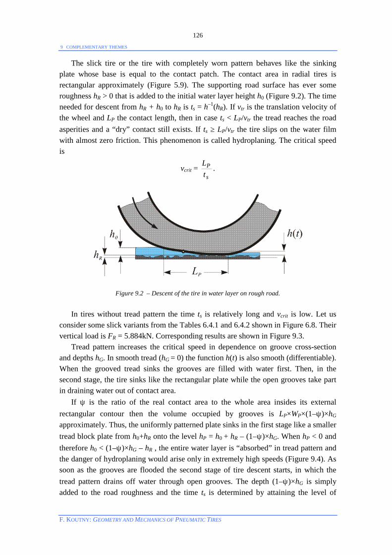
9 COMPLEMENTARY THEMES
F. KOUTNY: GEOMETRY AND MECHANICS OF PNEUMATIC TIRES
126
The slick tire or the tire with completely worn pattern behaves like the sinking plate whose base is equal to the contact patch. The contact area in radial tires is rectangular approximately (Figure 5.9). The supporting road surface has ever some roughness hR > 0 that is added to the initial water layer height h0 (Figure 9.2). The time needed for descent from hR + h0 to hR is ts = h–1(hR). If vtr is the translation velocity of the wheel and LP the contact length, then in case ts < LP/vtr the tread reaches the road asperities and a “dry” contact still exists. If ts ≥ LP/vtr the tire slips on the water film with almost zero friction. This phenomenon is called hydroplaning. The critical speed is
vcrit = s
PtL
.
Figure 9.2 – Descent of the tire in water layer on rough road. In tires without tread pattern the time ts is relatively long and vcrit is low. Let us consider some slick variants from the Tables 6.4.1 and 6.4.2 shown in Figure 6.8. Their vertical load is FR = 5.884kN. Corresponding results are shown in Figure 9.3. Tread pattern increases the critical speed in dependence on groove cross-section and depths hG. In smooth tread (hG = 0) the function h(t) is also smooth (differentiable). When the grooved tread sinks the grooves are filled with water first. Then, in the second stage, the tire sinks like the rectangular plate while the open grooves take part in draining water out of contact area. If ψ is the ratio of the real contact area to the whole area insides its external rectangular contour then the volume occupied by grooves is LP×WP×(1–ψ)×hG approximately. Thus, the uniformly patterned plate sinks in the first stage like a smaller tread block plate from h0+hR onto the level hP = h0 + hR – (1–ψ)×hG. When hP < 0 and therefore h0 < (1–ψ)×hG – hR , the entire water layer is “absorbed” in tread pattern and the danger of hydroplaning would arise only in extremely high speeds (Figure 9.4). As soon as the grooves are flooded the second stage of tire descent starts, in which the tread pattern drains off water through open grooves. The depth (1–ψ)×hG is simply added to the road roughness and the time ts is determined by attaining the level of
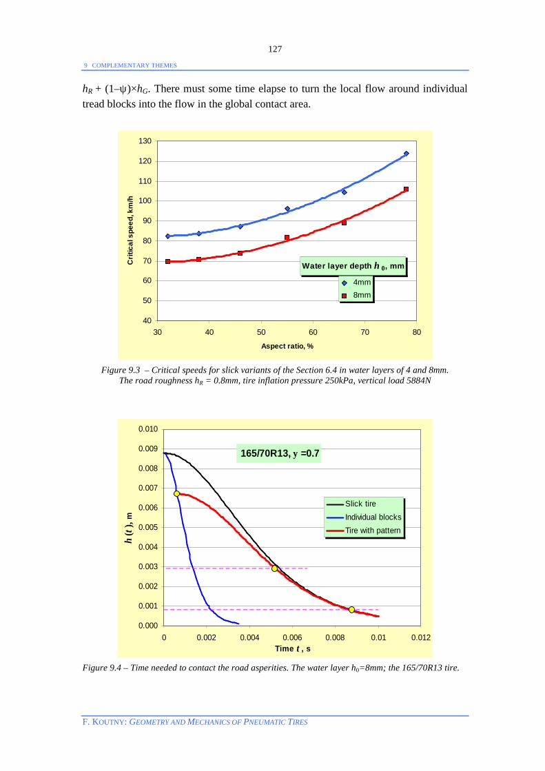
9 COMPLEMENTARY THEMES
F. KOUTNY: GEOMETRY AND MECHANICS OF PNEUMATIC TIRES
127
hR + (1–ψ)×hG. There must some time elapse to turn the local flow around individual tread blocks into the flow in the global contact area.
Water layer depth h 0, mm
40
50
60
70
80
90
100
110
120
130
30 40 50 60 70 80
Aspect ratio, %
Crit
ical
spe
ed, k
m/h
4mm 8mm
Figure 9.3 – Critical speeds for slick variants of the Section 6.4 in water layers of 4 and 8mm.
The road roughness hR = 0.8mm, tire inflation pressure 250kPa, vertical load 5884N
165/70R13, ψ =0.7
0.000
0.001
0.002
0.003
0.004
0.005
0.006
0.007
0.008
0.009
0.010
0 0.002 0.004 0.006 0.008 0.01 0.012Time t , s
h(t
), m
Slick tireIndividual blocksTire with pattern
Figure 9.4 – Time needed to contact the road asperities. The water layer h0=8mm; the 165/70R13 tire.

9 COMPLEMENTARY THEMES
F. KOUTNY: GEOMETRY AND MECHANICS OF PNEUMATIC TIRES
128
The impact of tread pattern grooves on the critical speed vcrit = LP/ts is shown in more detailed way in Figure 9.5. The formula (9.1) for h(t) reflects the influence of liquid density too. As the rain starts, the dust on highway turns into mud which has higher density than water. Figure 9.5 shows on a slick tire that the time needed for tire/road contact is increased and, consequently, the critical speed may decrease substantially.
1 2 4 8 160
4020406080
100120140160
180
200Crit. speed, km/h
Water layer h0 , mm
Groove h G , mm
Tire 165/70R13, h R =0.8mm
180-200160-180140-160120-140100-12080-10060-8040-6020-400-20
Figure 9.5 – Critical speeds for the 165/70R13 tire. Conditions p = 200kPa, F=3.15kN, ψ=0.7.
165/70R13, slick
0
0.001
0.002
0.003
0.004
0.005
0.006
0.007
0.008
0.009
0 0.005 0.01 0.015 0.02 0.025Time t , s
h(t
) , m Water
Mud
Figure 9.6 – Time needed to contact the road asperities; p = 200kPa, F=3.15kN.
Mud is assumed to have 4times higher density than water.
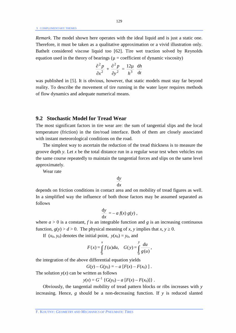
9 COMPLEMENTARY THEMES
F. KOUTNY: GEOMETRY AND MECHANICS OF PNEUMATIC TIRES
129
Remark. The model shown here operates with the ideal liquid and is just a static one. Therefore, it must be taken as a qualitative approximation or a vivid illustration only. Bathelt considered viscose liquid too [62]. Tire wet traction solved by Reynolds equation used in the theory of bearings (µ = coefficient of dynamic viscosity)
2
2
xp
∂
∂ + 2
2
yp
∂
∂ = 312h
µ th
dd
was published in [5]. It is obvious, however, that static models must stay far beyond reality. To describe the movement of tire running in the water layer requires methods of flow dynamics and adequate numerical means.
9.2 Stochastic Model for Tread Wear The most significant factors in tire wear are: the sum of tangential slips and the local temperature (friction) in the tire/road interface. Both of them are closely associated with instant meteorological conditions on the road. The simplest way to ascertain the reduction of the tread thickness is to measure the groove depth y. Let x be the total distance run in a regular wear test when vehicles run the same course repeatedly to maintain the tangential forces and slips on the same level approximately. Wear rate
xy
dd
depends on friction conditions in contact area and on mobility of tread figures as well. In a simplified way the influence of both those factors may be assumed separated as follows
xy
dd = – a f(x) g(y) ,
where a > 0 is a constant, f is an integrable function and g is an increasing continuous function, g(y) > d > 0. The physical meaning of x, y implies that x, y ≥ 0. If (x0, y0) denotes the initial point, y(x0) = y0, and
∫∫ ==yx
ugduyGduufxF
00 )()(,)()( ,
the integration of the above differential equation yields G(y) – G(y0) = – a [F(x) – F(x0) ] .
The solution y(x) can be written as follows y(x) = G–1 G(y0) – a [F(x) – F(x0)] .
Obviously, the tangential mobility of tread pattern blocks or ribs increases with y increasing. Hence, g should be a non-decreasing function. If y is reduced slanted
9 COMPLEMENTARY THEMES
F. KOUTNY: GEOMETRY AND MECHANICS OF PNEUMATIC TIRES
130
groove walls increase the tread pattern stiffness as well as the real tire/road contact interface. The simplest choice of g is then a polynomial of the second degree. Moreover, it must be expected that g tends to a constant if y is small, thus
2)0(
yg
dd2
= 0 .
Then g(y) = b0 + by2, b ≥ 0. Let it be simply put b0 = 1, i.e. g(y) = 1 + by2 .
Substituting this in the above equations gives
∫ +=
y
ubduyG
02)(1
)( = b
1 arctan ( b y) for b > 0,
G(y) = y for b = 0 and
y(x; a, b) =
=−−
>−−
0)]()([
0)]()([)(arctantan1
00
00
bxFxFay
bxFxFbaybb
for .
The function F is connected with the external conditions, especially those of weather. Its choice is a more delicate matter. Temperature and humidity are the most obvious characteristics of weather. Analysis of meteorological data records unveiled a considerable correlation between relative humidity and temperature of the air (in the Middle Europe area at least [64]). Both the quantities may be decomposed into periodic components determined by the instant position of the Earth on its orbit around the Sun and the stochastic ones, which can be considered to be normally distributed [11]. Autocorrelation functions showed that the stochastic component u at the sampling period of a day may be considered as a Markov process (autoregressive process AR(1))
u(k) = q u(k–1) + e(k), 0 < q < 1, k = 1, 2, … The random quantity e belongs to the normal distribution, e∈N(0, (1 – q2) var u) [11]. Using the process u for determining the values F(x) requires a convenient choice of its parameters. Data analysis led to values
q = 0.78, su ≈ uvar ≈ 0.19. If v is the average distance run each day,
v = Nx ,
then
var F x F x( ) ( )− 0 = v2 var ∑=
N
iiu
1)( ,
where N is the number of steps (days). It can be shown [64] that

9 COMPLEMENTARY THEMES
F. KOUTNY: GEOMETRY AND MECHANICS OF PNEUMATIC TIRES
131
var )()( 0xFxF − = var u vq
2
21( )−[ ])1(2)1( 2 NqqqN −−− ,
i.e. the variance is an increasing function of N. The relation
F x F x f u dut
t N
( ) ( ) ( )− −+
∫00
0
= 1.96 )()(var 0xFxF − ,
can be used in modeling the wear process. Here 1.96 = u0.975 is the critical value of normal distribution on the significance level of 0.05 [11]. The function f representing the weather (temperature) is [64]
f(t) = 1 – 0.14 cos (24.365
2 tπ + 0.019) + u(trunc(t)) ,
where trunc(t) denotes the entire part of t (e.g. trunc(π) = 3). Summarized up, the function y depends on two parameters a, b. But there is an obstacle in finding their estimates by regression: heteroscedasticity. On the other hand the minimization of the sum of equal powers of residuals is always a well defined problem and its solution may be found using direct methods [10]. In praxis tread wear tests are performed on homogenous sets of tires mounted with designed exchanges in a vehicle convoy that runs along a constant route. The depths of pattern grooves are measured and recorded periodically. This way a data set
(xi, yij) : i = 1, …, N; j = 1, .., Ji is obtained, where N is the number of distances at which the measurement was performed and Ji is the number of tires in ith measurement (Ji is usually the same for all i, nevertheless also the possibility of tire failure needs to be respected). Let
S(a, b; p) = ∑ ∑= =
−N
i
J
j
pijii
iybaxyw
1 1),;( ,
where p > 0 and wi are weights that shall express the importance of ith measurement, e.g.
wi =r
N
ixx
, r > 0,
to emphasize the last ones. The function S may be geometrically interpreted as a distance of the measurement point (y11, …,
11Jy , …, 1Ny , …, 1JNy ) from the hypersurface
H = y(xk; a, b) : k = 1, …, J1, J1+1, …, J1+J2, …, J1+ …+JN–1, …, n; –∞ < a, b < ∞
in the Euclidean space Rn, where n = iN
iJ∑
=1 is the total number of measurements
[9,64,65]. Direct search methods have proved to be most reliable for finding the parameters a, b.
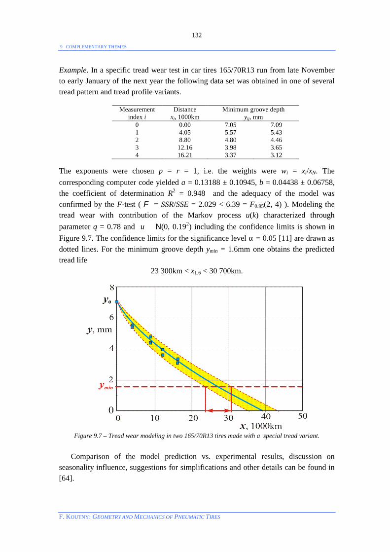
9 COMPLEMENTARY THEMES
F. KOUTNY: GEOMETRY AND MECHANICS OF PNEUMATIC TIRES
132
Example. In a specific tread wear test in car tires 165/70R13 run from late November to early January of the next year the following data set was obtained in one of several tread pattern and tread profile variants.
Measurement index i
Distance xi, 1000km
Minimum groove depth yij, mm
0 0.00 7.05 7.09 1 4.05 5.57 5.43 2 8.80 4.80 4.46 3 12.16 3.98 3.65 4 16.21 3.37 3.12
The exponents were chosen p = r = 1, i.e. the weights were wi = xi/xN. The corresponding computer code yielded a = 0.13188 ± 0.10945, b = 0.04438 ± 0.06758, the coefficient of determination R2 = 0.948 and the adequacy of the model was confirmed by the F-test ( F = SSR/SSE = 2.029 < 6.39 = F0.95(2, 4) ). Modeling the tread wear with contribution of the Markov process u(k) characterized through parameter q = 0.78 and u ∈ N(0, 0.192) including the confidence limits is shown in Figure 9.7. The confidence limits for the significance level α = 0.05 [11] are drawn as dotted lines. For the minimum groove depth ymin = 1.6mm one obtains the predicted tread life
23 300km < x1.6 < 30 700km.
Figure 9.7 – Tread wear modeling in two 165/70R13 tires made with a special tread variant.
Comparison of the model prediction vs. experimental results, discussion on seasonality influence, suggestions for simplifications and other details can be found in [64].
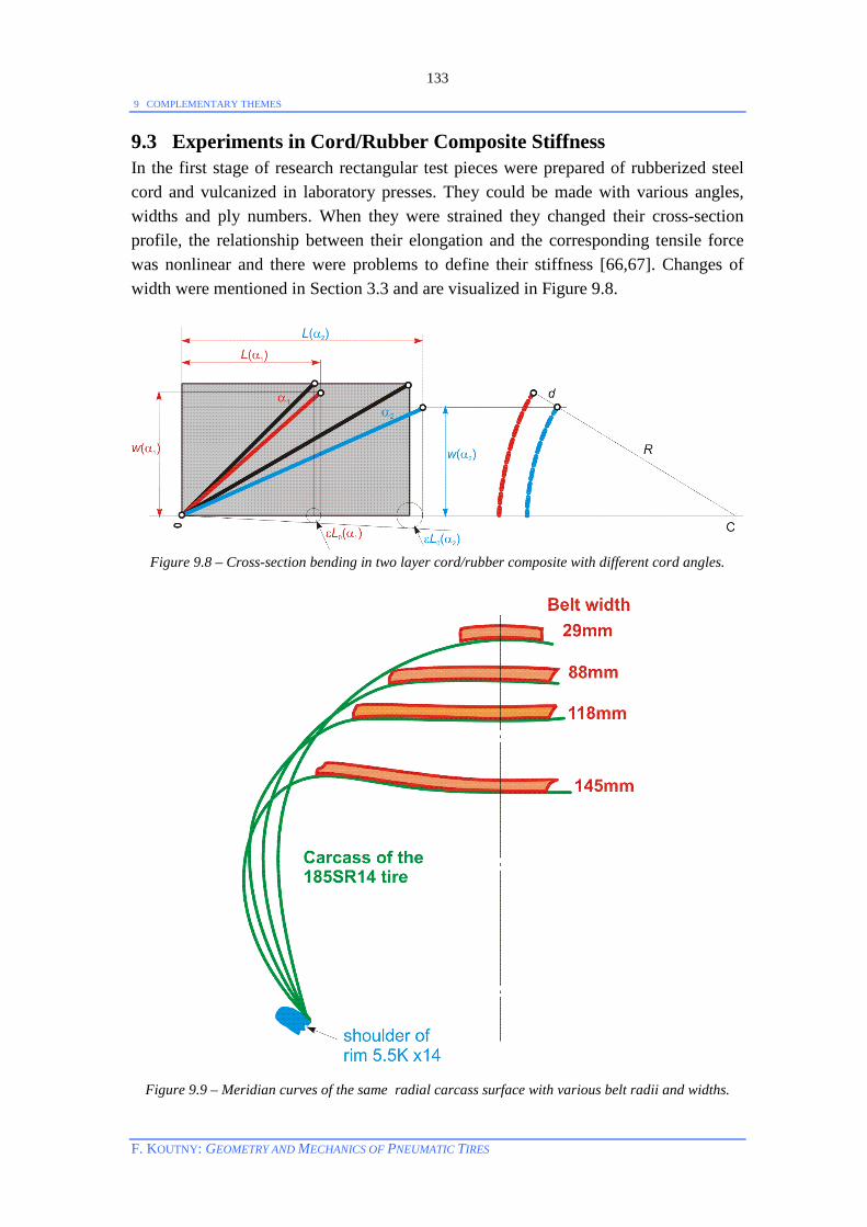
9 COMPLEMENTARY THEMES
F. KOUTNY: GEOMETRY AND MECHANICS OF PNEUMATIC TIRES
133
9.3 Experiments in Cord/Rubber Composite Stiffness In the first stage of research rectangular test pieces were prepared of rubberized steel cord and vulcanized in laboratory presses. They could be made with various angles, widths and ply numbers. When they were strained they changed their cross-section profile, the relationship between their elongation and the corresponding tensile force was nonlinear and there were problems to define their stiffness [66,67]. Changes of width were mentioned in Section 3.3 and are visualized in Figure 9.8.
Figure 9.8 – Cross-section bending in two layer cord/rubber composite with different cord angles.
Figure 9.9 – Meridian curves of the same radial carcass surface with various belt radii and widths.
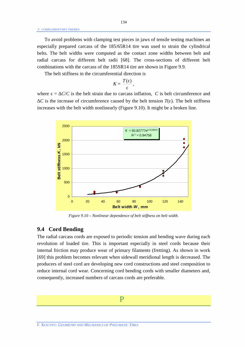
9 COMPLEMENTARY THEMES
F. KOUTNY: GEOMETRY AND MECHANICS OF PNEUMATIC TIRES
134
To avoid problems with clamping test pieces in jaws of tensile testing machines an especially prepared carcass of the 185/65R14 tire was used to strain the cylindrical belts. The belt widths were computed as the contact zone widths between belt and radial carcass for different belt radii [68]. The cross-sections of different belt combinations with the carcass of the 185SR14 tire are shown in Figure 9.9. The belt stiffness in the circumferential direction is
K = εε)(T ,
where ε = ∆C/C is the belt strain due to carcass inflation, C is belt circumference and ∆C is the increase of circumference caused by the belt tension T(ε). The belt stiffness increases with the belt width nonlinearly (Figure 9.10). It might be a broken line.
K = 50.82777e0.02380W
R 2 = 0.94758
0
500
1000
1500
2000
2500
0 20 40 60 80 100 120 140Belt width W , mm
Bel
t stif
fnes
s K
, kN
Figure 9.10 – Nonlinear dependence of belt stiffness on belt width.
9.4 Cord Bending The radial carcass cords are exposed to periodic tension and bending wave during each revolution of loaded tire. This is important especially in steel cords because their internal friction may produce wear of primary filaments (fretting). As shown in work [69] this problem becomes relevant when sidewall meridional length is decreased. The producers of steel cord are developing new cord constructions and steel composition to reduce internal cord wear. Concerning cord bending cords with smaller diameters and, consequently, increased numbers of carcass cords are preferable.
P

REFERENCES
F. KOUTNY: GEOMETRY AND MECHANICS OF PNEUMATIC TIRES
135
REFERENCES Note: All papers published in Plasty a kaučuk are in Czech. [1] TOMKINS, E.: "The History of the Pneumatic Tyre". Eastland Press, London 1981. [2] HOFFERBERTH, W., "Zur Statik des Luftreifens", Kautschuk u. Gummi, 9, 1956, S. 225. [3] BIDERMAN, V. L. in: "Trudy NIIŠP", sb. 3, Moscow 1957. [4] FRANK, F. – HOFFERBERTH, W., Rubber Chemistry and Technology, 40, 1967, p. 271.
[5] BIDERMAN, V. L. – BUKHIN, B. L. et al.: "Mechanics of Pneumatic Tires I" (Russian), Moscow 1974.
[6] BUKHIN, B. L. et al.: "Mechanics of Pneumatic Tires II" (Russian), Moscow 1976.
[7] "Mechanics of Pneumatic Tires", editor S. K. CLARK, U.S. Government Printing Office, Washington, D. C. 1981.
[8] GENT, A. N. – WALTER, J. D. et al.: "The Pneumatic Tire". NHTSA Washington 2005.
[9] www.koutny-math.com (Courses | Mathematical Base for Applications). [10] www.koutny-math.com (Courses | Numerical Methods & Fourier Analysis). [11] www.koutny-math.com (Courses | Prelude to Probability and Statistics). [12] KOUTNY, F., "A Method for Computing the Radial Deformation Characteristics of Radial Tires", Tire Science and Technology, 4, 1976, p. 190.
[13] RHYNE, T. B., Tire Science and Technology, 33, 2005, pp. 136-155.
[14] MEISSNER, B. – ZILVAR, V.: "Physics of Polymers". SNTL, Prague 1987.
[15] KOUTNÝ, F. – KUSÁK, K., "Nonlinearity of Rubber Shear Strain ", Yearbook VÚGPT ´82, 1982, p. 46.
[16] KOUTNÝ, F. – KUSÁK, K., "On Small Strains in Rubber", Plasty a kaučuk, 21, 1984, p. 296.
[17] KOUTNÝ, F. – SYCHA, A., "Notes on Radial Tires Rubber Proprieties ", Plasty a kaučuk, 25, 1988, p. 292.
[18] KOUTNÝ, F., "Viscoelastic Properties of Nylon Cords", Plasty a kaučuk, 27, 1990, p. 139. [19] KOUTNÝ, F., "Water-Filled Tire", Plasty a kaučuk, 19, 1982, p. 311. [20] KOUTNÝ, F., "Simpson’s Formula in Computing Building Drum Width", Plasty a kaučuk, 3, 1966, p. 208. [21] LEIBEE, J. B. – SCHAFFERS, W. J., "A New Tire Expansion Rule and its Use in Tire Design Computations", Rubber Chemistry and Technology, 42, 1969, p. 1079.
REFERENCES
F. KOUTNY: GEOMETRY AND MECHANICS OF PNEUMATIC TIRES
136
[22] KOUTNY, F., "Mathematische Untersuchung der Beziehungen zwischen den Konfektionsgrößen eines Autoreifens I", Plaste u. Kautschuk, 14, 1967, S. 327. [23] KOUTNY, F., " Mathematische Analyse der Beziehungen zwischen den Konfektionsgrößen von Kraftfahrzeugen II", Plaste u. Kautschuk, 16, 1969, S. 353. [24] KOUTNY, F.: "Air Volume Energy Method in Theory of Tires". International Polymer Science and Technology, 5, 1978, No. 8/T100.
[25] BIDERMAN, V. L. et al.: "Atlas of Pneumatic Tires Equilibrium Shapes Nomographs”. Moscow 1967.
[26] KOUTNY, F., "Meridian des aufgepumpten Reifens I", Plaste u. Kautschuk, 18, 1971, S. 282. [27] KOUTNY, F., "Meridian des aufgepumpten Reifens II", Plaste u. Kautschuk, 18, 1971, S. 680. [28] KOUTNY, F., "Mathematical Methods in the Theory of Tires"(Czech), Plastikářský bulletin, 1976, p. 165. [29] KOUTNÝ, F., "Calculations for Cross-Ply Tires I ", International Polymer Science and Technology, 9, 1982, No. 5/T65. [30] KOUTNY, F., "Calculations for Cross-Ply Tires II ", International Polymer Science and Technology, 9, 1982, No. 2/T67. [31] FRANK, F. - ELLIS, J.R.: A.S.A.E. Report No. 2, September 1966. [32] www.tufo.com [33] KOUTNÝ, F., "Pneumatic Toroidal Springs" (Czech), Strojnícky časopis, 33, 1982, p. 477. [34] KOUTNY, F., "Über die Druckexpansion der Radialkarkasse beim Aufbau", Kautschuk + Gummi, Kunststoffe, 35, 1982, S. 501 [35] KOUTNÝ, F., "Geometry of a Cordless Tire ", Plasty a kaučuk, 8, 1971, p. 110. [36] JANDIK, M. – KOUTNY, F., "Nomograms for Equilibrium Profiles of Radial Tyres", International Polymer Science and Technology, 1, 1974, No. 5/T75. [37] KOUTNY, F., "Static Calculations of Radial Tires", Plasty a kaučuk, 10, 1973, p. 360. [38] KOUTNÝ, F., "Static Belt Tension in Belted Tires", Plasty a kaučuk, 8, 1971, p. 365. [39] www.koutny-math.com (Miscellany | Strength). [40] ODSTRČIL, J. – KOUTNÝ, F.: Introductory Study to Tire Vibrations" (Czech). VÚGPT Report No. 695. Zlín 1968. [41] KOUTNÝ, F., "Elastic Behavior of Car Tires. Measurement of Radial Stiffness" (Czech). VÚGPT Report No. 813/6, Zlín 1969.

REFERENCES
F. KOUTNY: GEOMETRY AND MECHANICS OF PNEUMATIC TIRES
137
[42] KOUTNY, F., "Load-Deflection Curves for Radial Tyres", Applied Mathematical Modelling, 5, 1981, p. 422. [43] KOUTNY, F., "Cornering radial tyres", Applied Mathematical Modelling, 7, 1983, p. 139. [44] BRDIČKA, M. – HLADÍK, A.: "Theoretical Mechanics". Academia, Prague 1987. [45] GREGUŠ, M. – ŠVEC, M. – ŠEDA, V.: "Ordinary Differential Equations" (Slovak), ALFA Bratislava 1985. [46] ZIKA, V. – KOUTNY, F., "Use of Fourier Analysis for Designing Tyre Treads", International Polymer Science and Technology, 15, 1988, No. 3, T/50. [47] LANDAU, L. D. – LIFSHITZ, E. M.: "Theory of Elasticity. Theoretical Physics VII" (Russian). Moscow 1965. [48] WESTERMANN, S. – PETRY, F. – THIELEN, G.: "Impact of Fundamental Contact Mechanics on Development ", Tire Technology International, The Annual Review 2004, p. 68. [49] FEYNMAN, R., P. – LEIGHTON, R. B. – SANDS, M.: The Feynman Lectures on Physics (Chapter 12). Addison-Wesley, 1966. [50] KOUTNÝ, F., "On Dynamic Behavior of Radial Tires", Plasty a kaučuk, 32, 1995, p. 262. [51] LÁZNIČKA, L., "Construction and Properties of Radial Tires" (Czech), PhD Thesis, UTB Zlin, 2007. [52] KOUTNY, F., "Analytical Comments on Radial Tires Nonuniformity ", Tire Science and Technology, 24, 1996, pp. 132-152. [53] KOUTNY, F., "Gürtelreifengeometrie und ihre Konsequenzen", Kautschuk + Gummi, Kunststoffe, 31, 1978, S. 156. [54] ANDĚL, J., "Foundations of Mathematical Statistics," (in Czech) SNTL Prague 1978. [55] LÁZNIČKA, L. – KOUTNÝ, F., "Rolling Resistance in Truck Tires", Plasty a kaučuk, 41, 2004/No 11-12, p. 11. [56] KOUTNÝ, F., "Impact of Inflation Pressure and Load on Rolling Resistance of Radial Tires ", Plasty a kaučuk, 34, 1997, p. 4. [57] LÁZNIČKA, L. – KOUTNÝ, F., "Pneumatic Tire as a Vertical Dynamic Element in Vehicle", Plasty a kaučuk, 42, 2005/No 3-4, p. 8. [58] KOUTNY, F., "Stochastic Elements in the Carcass of a Radial Tyre", International Polymer Science and Technology, 6, 1979, No. 5, T/69. [59] KOUTNÝ, F., "Statistical Analysis of some Disturbances of Tire Uniformity ", Plasty a kaučuk, 16, 1979, s. 243. [60] KOUTNÝ, F. – LÁZNIČKA, L., "On Radial Uniformity of Tires ", Plasty a kaučuk, 42, 2005/No 7-8, p. 6. [61] KOUTNÝ, F. – LÁZNIČKA, L., "Quasistatic Uniformity of Tires – Distribution and Correlation", Plasty a kaučuk, 42, 2005/No 9-1, p. 8. [62] BATHELT, H., Zeitschrift für angewandte Mathematik und Mechanik, 53, 1973, S. 675.
REFERENCES
F. KOUTNY: GEOMETRY AND MECHANICS OF PNEUMATIC TIRES
138
[63] KOUTNY, F. – ZATLOUKAL, A., "Aquaplaning", International Polymer Science and Technology, 3, 1976, No. 10, T/92. [64] KOUTNY, F., "A Model for Tire Wear", Rubber Chemistry and Technology, 64, 1991, p. 683. [65] KOUTNÝ, F. – ČEVELÍK, R., "Nonlinear Regression in Physical Analyses of Polymers", Plasty a kaučuk, 26, 1990, p. 367. [66] KOUTNÝ, F., "Circumferential Stiffness of Tire Belts", Plasty a kaučuk, 10, 1973, p. 109. [67] KOUTNY, F. – SINDELAR, M., "Experimental Study of the Stiffness of the Cord- reinforced Rubber", International Polymer Science and Technology, 3, 1976, No. 10, T/92. [68] KOUTNY, F. – SYCHA, A. – MATUCHA, P., "Experimental Study of the Circumferential Stiffness of Tyre Belts", International Polymer Science and Technology, 6, 1979, No. 8, T/42. [69] KOUTNY, F., "Bending Stress in the Cord of Radial-ply Tyres", International Polymer Science and Technology, 2, 1975, No. 12, T/7.
INDEX
F. KOUTNY: GEOMETRY AND MECHANICS OF PNEUMATIC TIRES
139
INDEX Air volume theory 23 amplitude specter in uniformity 108 Basic equation of the belt model 56 bead tension 50 belt axial oscillations 75 belt circumferential oscillations 75 belt displacements u, v, w 53 belt model 53 belt oscillations 73 belt radial oscillations 74 belt support stiffness coefficient ku, kv, kw 53 beta distribution, generalized 109 boundary conditions for belt model 58 building drum 15 Carcass 2 carcass cord tension 48 carcass expansion 15 carcass expansion 19 Clairaut’s equation 18 cord angle α(r) 15 cord azimuth 17 cord bending 134 cord hysteresis 9 cord length 17 cord path 15 cord properties 9 cord trajectory 16 cord/rubber composite stiffness 133 cornering 62 correlation among uniformity components 113 cosine expansion rule 20 critical speed, hydroplaning 126 Dependence of µ (RRC) on p, F 96 dependence of µ (RRC) on velocity 89 designing problem (A) 29 designing problem (B) 30 designing problems 28 diagonal tire, carcass 15 double-branch normal distribution 112 Energy distribution 11 equilibrium meridian curve 23 equilibrium shape 23 FEA 4 FEM 3 Fisher test in uniformity harmonics 108 friction 85 Generalized cosine rule 20 geodesic line 18 High-speed uniformity 115
hydroplaning 123 hysteresis loop 8 Inner liner 2 Linear expansion rule 21 linearly elastic membrane 40 Markov process 130 meridional stress 48 Nylon cord 9 Optimization problems 78 Radial carcass 22 radial carcass meridian 36 radial loading 59 radial tire 43 radial tire, problems (A), (B) 45 radial uniformity disturbances 102 resilience Lüpke 8 rim 2 road/drum incompatibility 77 rolling resistance 85 rolling resistance measurement 86 rolling resistance variability 87 rubber properties 6 Shear modulus 6 sidewall 2 sine expansion rule 20 solutions of belt model equations 57 standard uniformity distribution 109 steel cord 9 stiff eccentric model 116 stochastic tread wear model 129 stress calculations 46 Tangent expansion rule 20 tangential loadings 60 tire building parameters 22 tire parts 2 tire uniformity 99 total belt tension 48 transfer function 101 tread 2 tread influence in cornering 83 tubular tire theory 32 two-mass model of vehicle 99 Verification of belt model 65 Wheel oscillations 71 Young’s modulus 6