Weyl Geometry and the Nonlinear Mechanics ofDistributed Point Defects∗

Arash Yavari† Alain Goriely‡

25 July 2012

Abstract

In this paper we obtain the residual stress field of a nonlinear elastic solid with a spherically-symmetricdistribution of point defects. The material manifold of a solid with distributed point defects – where the bodyis stress-free – is a flat Weyl manifold, i.e. a manifold with an affine connection that has non-metricity withvanishing traceless part but both its torsion and curvature tensors vanish. Given a spherically-symmetricpoint defect distribution, we construct its Weyl material manifold using the method of Cartan’s movingframes. Having the material manifold the anelasticity problem is transformed to a nonlinear elasticityproblem; all one needs to calculate residual stresses is to find an embedding into the Euclidean ambientspace. In the case of incompressible neo-Hookean solids we calculate the residual stress field. We finallyconsider the example of a finite ball of radius Ro and a point defect distribution uniform in a ball of radiusRi < Ro and vanishing elsewhere. We show that the residual stress field inside the ball of radius Ri isuniform and hydrostatic. We also prove a nonlinear analogue of Eshelby’s celebrated inclusion problem fora spherical inclusion in an isotropic incompressible nonlinear solid.

1 Introduction

The stress field of a single point defect in an infinite linear elastic solid was obtained by Love [1927] almostninety years ago. He observed a 1/r3 singularity. For distributed defects, Eshelby [1954] showed that for abody with a uniform distribution of point defects, in the framework of linearized elasticity, the body expandsuniformly. In other words, a uniform distribution of point defects is stress-free (if the body is not constrainedon its boundaries)1. Such calculations for nonlinear solids have not been done to this date. In the linearelasticity setting, point defects are modeled as centers of expansion or contraction [Garikipati, et al., 2006]. Inthe nonlinear framework presented in this paper, we start with a distributed point defect and use non-metricityin the material manifold to model the effect of point defects.

It has been known for a long time that the mechanics of solids with distributed defects can be formulatedusing non-Riemannian geometries [Kondo, 1955a,b; Bilby, et al., 1955; Bilby and Smith, 1956]. In [Yavari andGoriely, 2012a] we presented a comprehensive theory of the mechanics of distributed dislocations based onRiemann-Cartan geometry. We showed that in the geometric framework several examples of residual stressfield of solids with distributed dislocations can be solved analytically. We calculated the residual stress fieldof several examples analytically. Later in [Yavari and Goriely, 2012b], we extended the geometric theory tothe mechanics of solids with distributed disclinations. In the case of both dislocations and disclinations thereare exact solutions in the framework of nonlinear elasticity [Rosakis and Rosakis, 1988; Zubov, 1997; Acharya,2001].

While it has been noted that the geometric object relevant to point defects is non-metricity [Falk, 1981; deWit, 1981; Grachev, et al., 1989; Kroner, 1990; Miri and Rivier, 2002], there are no exact nonlinear solutions forpoint defects in the literature. In other words, the coupling between the geometry and the mechanics of pointdefects is missing. The purpose of this paper is to develop a fully geometric and exact (in the sense of elasticity)

∗To appear in the Proceedings of The Royal Society A.†School of Civil and Environmental Engineering, Georgia Institute of Technology, Atlanta, GA 30332, USA. E-mail:

arash.yavari@ce.gatech.edu.‡OCCAM, Mathematical Institute, University of Oxford, Oxford, OX1 3LB, UK.1We show in this paper that for an incompressible nonlinear solid this result still holds.

1

2 Non-Riemannian Geometries and Cartan’s Moving Frames 2

theory of distributed point defects. As an application of this geometric theory, we obtain the stress field of aspherically-symmetric distribution of point defects in a neo-Hookean solid. We also prove a nonlinear analogueof Eshelby’s celebrated inclusion problem for a spherical inclusion in an isotropic incompressible nonlinear solid.

This paper is structured as follows. In §2 we briefly review some basic definitions and concepts from differ-ential geometry and, in particular, Cartan’s moving frames and Weyl geometry. Kinematics and equations ofmotion for nonlinear elasticity and anelasticity are discussed in §3. In §4 we look at the problem of a spherically-symmetric distribution of point defects. Using Cartan’s structural equations we obtain an orthonormal coframefield and hence the material metric. We then make a connection between the material metric and the volumedensity of point defects using a compatible volume element in the Weyl material manifold. Having the materialmetric we then calculate the residual stress field. Next, we study an example of a point defect distributionuniform in a small ball and vanishing outside the ball. We show that for any isotropic incompressible nonlinearsolid the residual stress field inside the small ball is uniform. This is a nonlinear analogue of Eshelby’s celebratedinclusion problem. We then show that a uniform point defect distribution is the only spherically-symmetriczero-stress point defect distribution. Finally, we compare the linear and nonlinear solutions for the radial stressdistribution.

2 Non-Riemannian Geometries and Cartan’s Moving Frames

2.1 Riemann-Cartan manifolds

We tersely review some elementary facts about affine connections on manifolds and the geometry of Riemann-Cartan and Weyl manifolds. For more details see Schouten [1954]; Bochner and Yano [1952]; Nakahara [2003];Nester [2010]; Gilkey and Nikcevic [2011]; Hehl, et al. [1981]; Rosen [1982]. A linear (affine) connection on amanifold B is an operation ∇ ∶ X (B) × X (B) → X (B), where X (B) is the set of vector fields on B, such that∀ X,Y,X1,X2,Y1,Y2 ∈ X (B),∀ f, f1, f2 ∈ C∞(B),∀ a1, a2 ∈ R:

i) ∇f1X1+f2X2Y = f1∇X1Y + f2∇X2Y, (2.1)

ii) ∇X(a1Y1 + a2Y2) = a1∇X(Y1) + a2∇X(Y2), (2.2)

iii) ∇X(fY) = f∇XY + (Xf)Y. (2.3)

∇XY is called the covariant derivative of Y along X. In a local chart XA, ∇∂A∂B = ΓCAB∂C , where ΓCABare Christoffel symbols of the connection and ∂A = ∂

∂xAare natural bases for the tangent space corresponding

to a coordinate chart xA. A linear connection is said to be compatible with a metric G of the manifold if

∇X ⟨⟨Y,Z⟩⟩G = ⟨⟨∇XY,Z⟩⟩G + ⟨⟨Y,∇XZ⟩⟩G , (2.4)

where ⟨⟨., .⟩⟩G is the inner product induced by the metric G. It can be shown that ∇ is compatible with G ifand only if ∇G = 0, or in components

GAB∣C = ∂GAB∂XC

− ΓSCAGSB − ΓSCBGAS = 0. (2.5)

An n-dimensional manifold B with a metric G and a G-compatible connection ∇ is called a Riemann-Cartanmanifold [Cartan, 1924, 1955, 2001; Gordeeva, et al., 2010].

The torsion of a connection is defined as

T (X,Y) = ∇XY −∇YX − [X,Y]. (2.6)

In components in a local chart XA, TABC = ΓABC − ΓACB . ∇ is symmetric if it is torsion-free, i.e. ∇XY −∇YX = [X,Y]. On any Riemannian manifold (B,G) there is a unique linear connection ∇ that is compatiblewith G and is torsion-free. This is the Levi-Civita connection. In a manifold with a connection the curvatureis a map R ∶ X (B) ×X (B) ×X (B)→ X (B) defined by

R(X,Y)Z = ∇X∇YZ −∇Y∇XZ −∇[X,Y]Z, (2.7)

2.2 Cartan’s moving frames 3

or in components

RABCD = ∂ΓACD∂XB

− ∂ΓABD∂XC

+ ΓABMΓMCD − ΓACMΓMBD. (2.8)

2.2 Cartan’s moving frames

Consider a frame field eαNα=1 that at every point of a manifold B forms a basis for the tangent space. Assumethat this frame is orthonormal, i.e. ⟨⟨eα,eβ⟩⟩G = δαβ . This is, in general, a non-coordinate basis for the tangentspace. Given a coordinate basis ∂A an arbitrary frame field eα is obtained by a GL(N,R)-rotation of ∂Aas eα = Fα

A∂A such that orientation is preserved, i.e. detFαA > 0. For the coordinate frame [∂A, ∂B] = 0 but

for the non-coordinate frame field we have

[eα,eα] = −cγαβeγ , (2.9)

where cγαβ are components of the object of anhonolomy. It can be shown that cγαβ = FαAFβ

B (∂AFγB − ∂BFγA),where FγB is the inverse of Fγ

B . The frame field eα defines the co-frame field ϑαNα=1 such that ϑα(eβ) = δαβ .The object of anholonomy is defined as cγ = dϑγ . Writing this in the coordinate basis we have

cγ = d (FγBdXB) = ∑α<β

cγαβϑα ∧ ϑβ . (2.10)

Connection 1-forms are defined as∇eα = eγ ⊗ ωγα. (2.11)

The corresponding connection coefficients are defined as ∇eβeα = ⟨ωγα,eβ⟩eγ = ωγβαeγ . In other words,

ωγα = ωγβαϑβ . Similarly, ∇ϑα = −ωαγϑγ , and ∇eβϑα = −ωαβγϑγ . In the non-coordinate basis torsion has the

following componentsTαβγ = ωαβγ − ωαγβ + cαβγ . (2.12)

Similarly, the curvature tensor has the following components with respect to the frame field

Rαβλµ = ∂βωαλµ − ∂λωαβµ + ωαβξωξλµ − ωαλξωξβµ + ωαξµcξβλ. (2.13)

In the orthonormal frame, metric has the simple representation G = δαβϑα ⊗ ϑβ .

2.3 Non-metricity and Weyl manifolds

Given a manifold with a metric and an affine connection (B,∇,G), non-metricity is a map Q ∶ X (B) ×X (B) ×X (B)→ X (B) defined as

Q(U,V,W) = ⟪∇UV,W⟫G + ⟪V,∇UW⟫G −U[⟪V,W⟫G]. (2.14)

In the frame eα, Qγαβ =Q(eγ ,eα,eβ).2 Non-metricity 1-forms are defined as Qαβ = Qγαβϑγ . It is straight-forward to show that

Qγαβ = ωξγαGξβ + ωξγβGξα − ⟨dGαβ ,eγ⟩ = ωβγα + ωαγβ − ⟨dGαβ ,eγ⟩, (2.15)

where d is the exterior derivative. Thus

Qαβ = ωαβ + ωβα − dGαβ =∶ −DGαβ , (2.16)

where D is the covariant exterior derivative. This is called Cartan’s zeroth structural equation. For an orthonor-mal frame Gαβ = δαβ and hence

Qαβ = ωαβ + ωβα. (2.17)

2Here, we mainly follow the notation of Hehl and Obukhov [2003].

2.4 The compatible volume element on a Weyl manifold 4

Weyl 1-form is defined as

Q = 1

nQαβGαβ . (2.18)

ThusQαβ = Qαβ +QGαβ , (2.19)

where Q is the traceless part of non-metricity. If Q = 0, (B,∇,G) is called a Weyl-Cartan manifold. In addition,if ∇ is torsion-free, (B,∇,G) is called a Weyl manifold. It can be shown that

Rαα = n2dQ. (2.20)

This implies that for a flat Weyl manifold dQ = 0. One can show that [Hehl, et al., 1995]

ωαα = n2Q + 1

2GαβdGαβ =

n

2Q + d ln

√detG. (2.21)

AlsoD

√detG = d

√detG − ωαα

√detG = −n

2Q√

detG, (2.22)

i.e. the connection ∇ is not volume-preserving.The torsion and curvature 2-forms are defined as

T α = dϑα + ωαβ ∧ ϑβ , (2.23)

Rαβ = dωαβ + ωαγ ∧ ωγβ . (2.24)

These are called Cartan’s first and second structural equations. In this framework, Bianchi identities then read:

DQαβ ∶= dQαβ − ωγα ∧Qγβ − ωγβ ∧Qαγ =Rαβ +Rβα, (2.25)

DT α ∶= dT α + ωαβ ∧ T β =Rαβ ∧ ϑβ , (2.26)

DRαβ ∶= dRαβ + ωαγ ∧Rγβ − ωγβ ∧Rαγ = 0. (2.27)

Note that for a flat manifold DT α = 0 and DQαβ = 0.

2.4 The compatible volume element on a Weyl manifold

Given a Weyl manifold one needs a volume element to be able to calculate volume of an arbitrary subset. Ourmotivation here is to have a natural way of measuring volumes in the material manifold and hence to be ableto calculate the volume density of point defects using the geometry of the Weyl material manifold. Here, bycompatible volume element we mean a volume element that has vanishing covariant derivative. The volumeelement of the underlying Riemannian manifold is not appropriate; we need a natural volume element in thesense of Saa [1995] (see also Mosna and Saa [2005]). A volume element on B is a non-vanishing n-form [Nakahara,2003]. In the orthonormal coframe field ϑα the volume form can be written as

µ = hϑ1 ∧ ... ∧ ϑn, (2.28)

for some positive function h to be determined. In a coordinate chart XA the volume form is written as

µ = h√

detG dX1 ∧ ... ∧ dXn. (2.29)

Divergence of an arbitrary vector field W on B can be defined using the Lie derivative as [Abraham, et al.,1988]

(DivW)µ = LWµ. (2.30)

On the other hand, divergence is also defined using the connection as

Div∇W =WA∣A =WA

,A + ΓAABWB . (2.31)

3 Geometric Nonlinear Elasticity and Anelasticity 5

According to Saa [1995] µ is compatible with ∇ if

LWµ = (WA∣A)µ, (2.32)

which is equivalent to

D (h√

detG) = 0. (2.33)

Using (2.22) we can write

D (h√

detG) = hD√

detG +√

detG dh = (dh − n2hQ)

√detG = 0. (2.34)

Thusdh

h= d lnh = n

2Q. (2.35)

In coordinate form this reads∂ lnh

∂XA= n

2QA, (2.36)

or∂h

∂XA− n

2hQA = 0. (2.37)

Remark 2.1. Note that a Weylian metric on B is given by the pair (G,Q) with the equivalence relation(G,Q) ∼ (eΛG,Q − dΛ) for an arbitrary smooth function Λ on B [Folland, 1970]. Now if Q = dΩ for somesmooth function Ω, then by choosing Λ = Ω we have

(G,Q) ∼ (eΩG,0). (2.38)

In other words, when the Weyl 1-form is exact there exists an equivalent Riemannian manifold (B, eΩG). In

the equivalent Riemannian manifold the volume form is enΩ2 µG, where µG is the standard Riemannian volume

form of G. The volume form enΩ2 µG is identical to Saa’s compatible volume element [Saa, 1995]. In this paper

we call (B, eΩG) and (B,G), the equivalent, and the underlying Riemannian manifolds, respectively.

3 Geometric Nonlinear Elasticity and Anelasticity

3.1 Kinematics of nonlinear elasticity

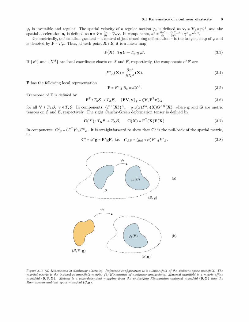
Let us first review a few of the basic notions of geometric nonlinear elasticity. A body B is identified with aRiemannian manifold B3 and a configuration of B is a mapping ϕ ∶ B → S, where S is another Riemannianmanifold [Marsden and Hughes, 1983; Yavari, et al., 2006], where the elastic body lives (see Fig. 3.1a). The setof all configurations of B is denoted by C. A motion is a curve c ∶ R→ C; t↦ ϕt in C. A fundamental assumptionis that the body is stress-free in the material manifold. It is the geometry of these two manifolds that describesany possible residual stresses.

For a fixed t, ϕt(X) = ϕ(X, t) and for a fixed X, ϕX(t) = ϕ(X, t), where X is position of material points inthe reference configuration B. The material velocity is given by

Vt(X) =V(X, t) = ∂ϕ(X, t)∂t

= d

dtϕX(t). (3.1)

Similarly, the material acceleration is defined by

At(X) =A(X, t) = ∂V(X, t)∂t

= d

dtVX(t). (3.2)

In components, Aa = ∂V a

∂t+ γabcV bV c, where γabc is the Christoffel symbol of the local coordinate chart xa.

Note that A does not depend on the connection coefficients of the material manifold. Here it is assumed that

3This is, in general, the underlying Riemannian manifold of the material manifold.

3.1 Kinematics of nonlinear elasticity 6

ϕt is invertible and regular. The spatial velocity of a regular motion ϕt is defined as vt = Vt ϕ−1t , and the

spatial acceleration at is defined as a = v = ∂v∂t+∇vv. In components, aa = ∂va

∂t+ ∂va

∂xbvb + γabcvbvc.

Geometrically, deformation gradient – a central object describing deformation – is the tangent map of ϕ andis denoted by F = Tϕ. Thus, at each point X ∈ B, it is a linear map

F(X) ∶ TXB → Tϕ(X)S. (3.3)

If xa and XA are local coordinate charts on S and B, respectively, the components of F are

F aA(X) = ∂ϕa

∂XA(X). (3.4)

F has the following local representationF = F aA ∂a ⊗ dXA. (3.5)

Transpose of F is defined byFT ∶ TxS → TXB, ⟪FV,v⟫g = ⟪V,FTv⟫G, (3.6)

for all V ∈ TXB, v ∈ TxS. In components, (FT(X))Aa = gab(x)F bB(X)GAB(X), where g and G are metrictensors on S and B, respectively. The right Cauchy-Green deformation tensor is defined by

C(X) ∶ TXB → TXB, C(X) = FT(X)F(X). (3.7)

In components, CAB = (FT)AaF aB . It is straightforward to show that C is the pull-back of the spatial metric,i.e.

C = ϕ∗g = F∗gF, i.e. CAB = (gab ϕ)F aAF bB . (3.8)

ϕt

ϕt

(S,g)

(S,g)

B

ϕt(B)

ϕt(B)

(B,∇,g)

(a)

(b)

Figure 3.1: (a) Kinematics of nonlinear elasticity. Reference configuration is a submanifold of the ambient space manifold. Themartial metric is the induced submanifold metric. (b) Kinematics of nonlinear anelasticity. Material manifold is a metric-affinemanifold (B,∇,G). Motion is a time-dependent mapping from the underlying Riemannian material manifold (B,G) into theRiemannian ambient space manifold (S,g).

3.2 Material manifold and anelasticity 7

3.2 Material manifold and anelasticity

In classical elasticity one starts with a stress-free configuration embedded in the ambient space and then makesthis embedding time-dependent (a motion), see Fig. 3.1a. In anelastic problems (anelastic in the sense ofEckart [1948]), the stress-free configuration is another manifold with a geometry explicitly depending on theanelasticity source(s), see Fig. 3.1b. The ambient space being a Riemannian manifold (S,g), the computationof stresses requires a Riemannian material manifold (B,G) (the underlying Riemannian material manifold) anda map ϕ ∶ B → S. For example, in the case of non-uniform temperature changes and bulk growth [Ozakinand Yavari, 2010; Yavari, 2010] one starts with a material metric G that specifies the relaxed distances of thematerial points. However, the material metric cannot always be obtained directly.

It turns out that for defects in solids, a metric-affine manifold can describe the stress-free configuration of thebody. In the case of dislocations, the material connection is flat, metric-compatible, and has a non-vanishingtorsion, which is identified with the dislocation density tensor, i.e. the material manifold is a Weitzenbockmanifold [Yavari and Goriely, 2012a]. Given a dislocation density tensor one can obtain the torsion of theaffine connection. Then using Cartan’s moving frames and structural equations one can find an orthonormalframe compatible with the torsion tensor. This, in turn, provides the material metric. Then, the computationof stress amounts to finding a mapping from the underlying Riemannian material manifold to the ambientspace manifold. In the case of disclinations, the physically relevant object is the curvature of a torsion-free andmetric-compatible connection and one can again find the metric using Cartan’s structural equations [Yavari andGoriely, 2012b].

For a solid with distributed point defects the material manifold is a Weyl manifold. Point defects affect thevolume of the stress-free configuration and this can be described using non-metricity with vanishing tracelesspart as will be shown shortly. The metric is obtained using Cartan’s structural equations and the compatiblevolume element of the Weyl material manifold. We conclude that all the anelastic effects can be embedded in theappropriate geometric characterization of the material manifold on which the computation of stresses reducesto a classical elasticity problem. This means that, in particular, the deformation gradient by construction ispurely elastic.

Remark 3.1. In a body with distributed point defects we expect the natural volume element to change frompoint to point (see Fig. 3.2) and this change of volume element is, in general, anisotropic. Weyl 1-form canmodel such an anisotropic change in the volume element. This is why the traceless part of non-metricity is notneeded in modeling distributed point defects.

Figure 3.2: In a Weyl manifold the Riemannian volume element varies from point to point.

3.3 Equations of motion

The internal energy density E (or free energy density Ψ) of a solid depends on the deformation gradient F.Since a scalar function of a two-point tensor must explicitly depend on both G and g, we have

E = E(X,N,Θ,F,G,g), Ψ = Ψ(X,Θ,F,G,g), (3.9)

where N and Θ are the specific entropy and absolute temperature, respectively.

4 Residual Stress Field of a Spherically-Symmetric Distribution of Point Defects 8

One can derive the equations of motion by either using an action principle or using covariance of energybalance [Marsden and Hughes, 1983; Yavari and Marsden, 2012]. For a motion ϕ ∶ B → S, where (B,G) and(S,g) are, respectively, the (underlying) Riemannian material and ambient space manifolds, the governingequations obtained as a consequence of the conservation of mass and balance of linear and angular momenta,in material form read

∂ρ0

∂t= 0, DivP + ρ0B = ρ0A, PFT = FPT, (3.10)

where ρ0, P,B, and A are the material mass density, the first Piola-Kirchhoff stress, the body force per unitundeformed volume (calculated using the Riemannian volume form), and the material acceleration, respectively.In components, the Cauchy equation (3.10)2 reads

∂P aA

∂XA+ ΓAABP

aB + γabcF bAP cA + ρ0Ba = ρ0A

a, (3.11)

where ΓABC are the Christoffel symbols of the material metric. Equivalently, in spatial coordinates

Lvρ = 0, divσ + ρb = ρa, σT = σ, (3.12)

where ρ, σ,b, and a are the spatial mass density, Cauchy stress, body force per unit deformed volume, and spatialacceleration, respectively. Lvρ is the Lie derivative of the mass density with respect to the (time-dependent)

spatial velocity. Note that σab = 1JP aAF bA, where J =

√detgdetG

detF is the Jacobian.

4 Residual Stress Field of a Spherically-Symmetric Distribution ofPoint Defects

As an application of the geometric theory, we revisit a classical problem of linear elasticity in the generalframework of exact nonlinear elasticity. Namely, we construct the material manifold of a spherically-symmetricdistribution of point defects in a ball of radius Ro, which is traction-free (or is under uniform pressure) on itsboundary sphere. The Weyl material manifold is then used to calculate the residual stress field.

4.1 The Weyl material manifold

In order to find a solution, we follow the procedure in [Adak and Sert, 2005; Yavari and Goriely, 2012a] andstart by an ansatz for the material coframe field. We then find a flat connection, which is torsion-free but hasa non-vanishing non-metricity compatible with the given point defect distribution. We do this using Cartan’sstructural equations and the compatible volume form of the Weyl material manifold. In the spherical coordinates(R,Θ,Φ), R ≥ 0, 0 ≤ Θ ≤ π, 0 ≤ Φ < 2π, let us look for a coframe field of the following form4

ϑ1 = f(R)dR, ϑ2 = RdΘ, ϑ3 = R sin Θ dΦ, (4.1)

for some unknown function f to be determined. We choose the following connection 1-forms

ω = [ωαβ] =⎛⎜⎜⎝

ω11 ω1

2 −ω31

−ω12 ω2

2 ω23

ω31 −ω2

3 ω33

⎞⎟⎟⎠, (4.2)

where

ω12 = −

1

Rϑ2, ω2

3 = −cot Θ

Rϑ3, ω3

1 =1

Rϑ3, ω1

1 = ω22 = ω3

3 = q(R)ϑ1, (4.3)

for a function q to be determined. This means that

Qαβ = 2δαβ q(R)ϑ1. (4.4)

4This construction is similar to that of Adak and Sert [2005]. Note that the Riemannian volume element is µG = ϑ1 ∧ϑ2 ∧ϑ3 =R2f(R) sin Θ dR ∧ dΘ ∧ dΦ, and hence f(R) > 0.

4.2 Volume density of point defects 9

We now need to enforce T α = 0. Note that

dϑ1 = 0, dϑ2 = 1

Rf(R)ϑ1 ∧ ϑ2, dϑ3 = − 1

Rf(R)ϑ3 ∧ ϑ1 + cot Θ

Rϑ2 ∧ ϑ3. (4.5)

From Cartan’s first structural equations we obtain

T 1 = 0, T 2 = [ 1

Rf(R) −1

R+ q(R)]ϑ1 ∧ ϑ2, T 3 = [ 1

Rf(R) −1

R+ q(R)]ϑ3 ∧ ϑ1. (4.6)

Therefore

q(R) = 1

R[1 − 1

f(R)] . (4.7)

It can be checked that for these connection 1-forms Rαβ = 0 are trivially satisfied. In this example the Weyl1-form is written as

Q = 2q(R)ϑ1 = 2

R[1 − 1

f(R)]ϑ1 = 2(f(R) − 1)

RdR. (4.8)

It is seen that dQ = 0 as is expected for a flat Weyl manifold.

4.2 Volume density of point defects

Consider a spherical shell of radius R and thickness ∆R. In the absence of point defects (Euclidean materialmanifold), the volume of this shell is

∆V0 = 2π∫π

0sin Θ dΘ∫

R+∆R

Rξ2dξ = 4π∫

R+∆R

Rξ2dξ. (4.9)

Now in the underlying Riemannian material manifold, the volume of the same spherical shell with point defectsis

∆VRiemannian = 2π∫π

0sin Θ dΘ∫

R+∆R

Rξ2f(ξ)dξ = 4π∫

R+∆R

Rξ2f(ξ)dξ. (4.10)

If there are only vacancies in this spherical shell (and no interstitials) we expect the volume of the Riemannianmaterial manifold to be smaller than ∆V0. In other words, for a distribution of vacancies we expect 0 < f(R) < 1.

In the presence of point defects the compatible volume element in the Weyl material manifold is written as

µ = h(R)ϑ1 ∧ ϑ2 ∧ ϑ3 = R2f(R)h(R) sin Φ dR ∧ dΘ ∧ dΦ, (4.11)

for some positive function h satisfying (2.36). In the Weyl material manifold the volume of the spherical shellof radius R and thickness ∆R is5

∆V = 2π∫π

0sin Θ dΘ∫

R+∆R

Rξ2f(ξ)h(ξ)dξ = 4π∫

R+∆R

Rξ2f(ξ)h(ξ)dξ. (4.12)

Total volume of defects in the spherical shell is ∆Vd = ∆V0 −∆V . Thus

∆Vd = 4π∫R+∆R

Rξ2[1 − f(ξ)h(ξ)]dξ. (4.13)

The volume density of point defects is defined as6

n(R) = lim∆R→0

∆Vd∆V0

= lim∆R→0

4π ∫R+∆RR ξ2[1 − f(ξ)h(ξ)]dξ

4πR2∆R= 1 − f(R)h(R). (4.14)

5Note that for the case of a spherically-symmetric point defect distribution as a consequence of the Poincare Lemma, Q = dΩ (seeRemark 3.2). In other words, we are calculating the volume of the equivalent Riemannian manifold of the Weyl material manifold.

6For a distribution of vacancies n(R) < 0 and for a distribution of interstitials n(R) > 0.

4.3 Residual stress calculation 10

Therefore

f(R) = 1 − n(R)h(R) . (4.15)

Note that f(R) > 0 and h(R) > 0 imply thatn(R) < 1. (4.16)

For our spherically-symmetric point defect distribution, the relationship (2.36) is simplified to read

d

dRlnh(R) = h

′(R)h(R) = 3(f(R) − 1)

R. (4.17)

From (4.15) and (4.17) we obtainRh′(R) + 3h(R) = 3(1 − n(R)). (4.18)

Hence

h(R) = 1 − 1

R3 ∫R

03y2n(y)dy. (4.19)

Therefore

f(R) = 1 − n(R)1 − 1

R3 ∫R

0 3y2n(y)dy. (4.20)

To check for consistency, let us consider a spherically-symmetric distribution of vacancies in a ball of radiusRo such that n(R) < 0 (h(R) > 1) and n′(R) > 0. For a distributed vacancy, we expect a smaller relaxed volume,i.e. µ0 > µG and hence f(R) < 1, where µ0 and µG are the volume forms of the flat Euclidean manifold andthe underlying Riemannian manifold, respectively. This can easily be verified using (4.20).

Example 4.1. If n(R) = n0, then f(R) = 1.

Remark 4.2. For an arbitrary distribution of point defects the defective solid is stress-free in a Weyl manifold(B,G,Q). Let us denote the volume form of the Weyl manifold by µ. For a subbody U ⊂ B, the volume of thevirgin (defect-free) and the defective subbody are

V0(U) = ∫Uµ0, V (U) = ∫

Uµ. (4.21)

The volume of the point defects in U is calculated as

Vd(U) = ∫Uµ0 − ∫U µ = ∫

U(µ0 −µ) = ∫U nµ0. (4.22)

This implies that n is the volume density of the point defects. Note that for vacancies Vd < 0.

4.3 Residual stress calculation

The material metric in spherical coordinates (R,Θ,Φ) has the following form:

G =⎛⎜⎝

f2(R) 0 00 R2 00 0 R2 sin2 Θ

⎞⎟⎠. (4.23)

We use the spherical coordinates (r, θ, φ) for the Euclidean ambient space with the following metric.

g =⎛⎜⎝

1 0 00 r2 00 0 r2 sin2 θ

⎞⎟⎠. (4.24)

In order to obtain the residual stress field we embed the material manifold into the ambient space. We look forsolutions of the form (r, θ, φ) = (r(R),Θ,Φ), and hence detF = r′(R). Assuming an incompressible solid, we

4.3 Residual stress calculation 11

have

J =√

detg

detGdetF = r2(R)

R2f(R)r′(R) = 1. (4.25)

Assuming that r(0) = 0 this gives us

r(R) = (∫R

03ξ2f(ξ)dξ)

13

. (4.26)

For a neo-Hookean material we have P aA = µF aBGAB − p (F −1)bAgab, where p = p(R) is the pressure field.

Thus

P =⎛⎜⎜⎜⎝

µR2

f(R)r2(R) −p(R)r2(R)f(R)R2 0 0

0 µR2 − p(R)

r2(R) 0

0 0 µR2 sin2 Θ

− p(R)r(R)2 sin2 Θ

⎞⎟⎟⎟⎠. (4.27)

Hence

σ =⎛⎜⎜⎜⎝

µR4

r4(R) − p(R) 0 0

0 µR2 − p(R)

r2(R) 0

0 0 1sin2 Θ

[ µR2 − p(R)

r2(R)]

⎞⎟⎟⎟⎠. (4.28)

In the absence of body forces, the only non-trivial equilibrium equation is σra∣a = 0 (p = p(R) is the consequenceof the other two equilibrium equations), which is simplified to read

σrr,r +2

rσrr − rσθθ − r sin2 θ σφφ = 0. (4.29)

Orr2

R2fσrr,R +

2

rσrr − 2rσθθ = 0. (4.30)

This then gives us

p′(R) = − 2µ

r(R)

⎡⎢⎢⎢⎢⎣f(R)( R

r(R))6

− 2( R

r(R))3

+ f(R)⎤⎥⎥⎥⎥⎦. (4.31)

Let us assume that the defective body is a ball of radius Ro. Assuming that the boundary of the ball istraction-free (σrr(Ro) = 0) we obtain

p(Ro) = µR4o

r4(Ro). (4.32)

Therefore, the pressure at all points inside the ball is

p(R) = µ R4o

r4(Ro)+ 2µ∫

Ro

R[f(ξ) ξ6

r7(ξ) − 2ξ3

r4(ξ) +f(ξ)r(ξ) ]dξ, (4.33)

and the radial stress is

σrr(R) = −2µ∫Ro

R[f(ξ) ξ6

r7(ξ) − 2ξ3

r4(ξ) +f(ξ)r(ξ) ]dξ

+µ [ R4

r4(R) −R4o

r4(Ro)] . (4.34)

For a given point defect distribution n(R), f(R) is obtained using (4.20). Pressure and stress are then calculatedby substituting f(R) into (4.33) and (4.34), respectively.

Remark 4.3. When n(R) = n0, we saw that f(R) = 1. This then implies that r(R) = R and p(R) = µ, i.e. thispoint defect distribution is stress-free. Eshelby [1954] showed this in the linearized setting. We will show in §4.4that this is the only zero-stress spherically-symmetric point defect distribution.

4.3 Residual stress calculation 12

Remark 4.4. We can calculate the stress field for the case when on the boundary of the body tractions arenon-zero. Assuming that P rR(Ro) = −p∞, we have

σrr(R) = −2µ∫Ro

R[f(ξ) ξ6

r7(ξ) − 2ξ3

r4(ξ) +f(ξ)r(ξ) ]dξ

+µ [ R4

r4(R) −R4o

r4(Ro)] − p∞

f(Ro)R2o

r2(Ro). (4.35)

Example 4.5. Let us consider the following point defect distribution7

n(R) =⎧⎪⎪⎨⎪⎪⎩

n0 0 ≤ R ≤ Ri,0 R > Ri,

(4.36)

where Ri < Ro. Thus

0 ≤ R ≤ Ri ∶ f(R) = 1, (4.37)

R > Ri ∶ f(R) = 1

1 − n0 (RiR

)3. (4.38)

Also

0 ≤ R ≤ Ri ∶ r(R) = R, (4.39)

R > Ri ∶ r(R) = [R3 + n0R3i ln((R/Ri)3 − n0

1 − n0)]

13

. (4.40)

Note that for 0 ≤ R ≤ Ri:

p(R) = µ R4o

r4(Ro)+ 2µ∫

Ro

Ri[f(ξ) ξ6

r7(ξ) − 2ξ3

r4(ξ) +f(ξ)r(ξ) ]dξ = pi, (4.41)

i.e. pressure is uniform and consequently σrr = µ − pi is uniform. Fig. 4.1 shows the distribution of P rR in theinterval [Ri,Ro] for different vacancy distributions and when Ro = 10Ri.

0.2 0.4 0.6 0.8 1.0

0.02

0.04

0.06

0.08

0.10

0.12

0.14

PrR

μ

n0 = -0.1n0 = -0.05

n0 = -0.02n0 = -0.01

R/R0

Figure 4.1: P rR distributions for Ri = Ro/10 and different values of n0.

Remark 4.6. The other two stress components are also equal to µ − pi in the ball R ≤ Ri. To see this, note

7Note that the total volume of point defects is ( 4π3R3i )n0.

4.4 Zero-stress spherically-symmetric point defect distributions 13

that in curvilinear coordinates, the components of a tensor may not have the same physical dimensions. Thefollowing relation holds between the Cauchy stress components (unbarred) and its physical components (barred)[Truesdell, 1953]

σab = σab√gaagbb no summation on a or b. (4.42)

The spatial metric in spherical coordinates has the form diag(1, r2, r2 sin2 θ), and this means that the nonzeroCauchy stress components are

σrr = σrr = µ R4

r4(R) − p(R), σθθ = r2σθθ = µr2(R)R2

− p(R),

σφφ = r2 sin2 θ σφφ = µr2(R)R2

− p(R). (4.43)

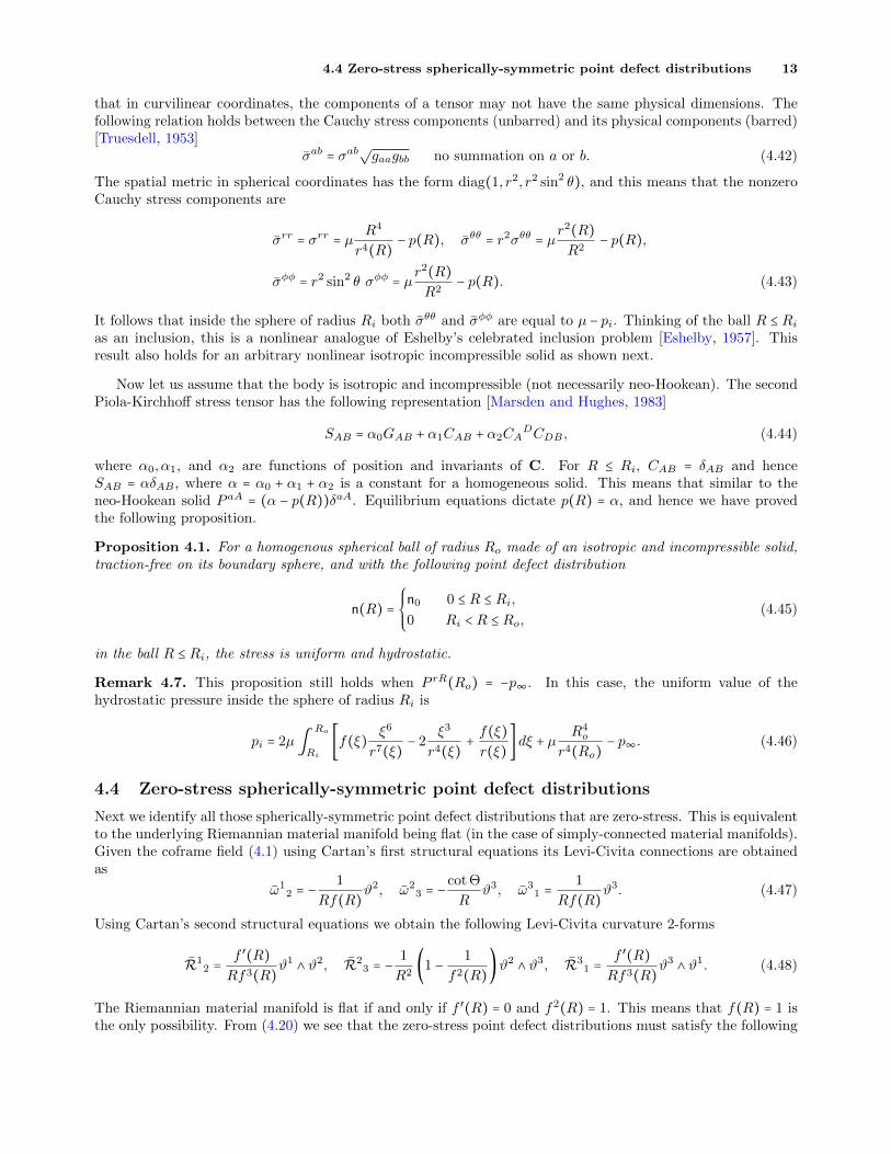
It follows that inside the sphere of radius Ri both σθθ and σφφ are equal to µ − pi. Thinking of the ball R ≤ Rias an inclusion, this is a nonlinear analogue of Eshelby’s celebrated inclusion problem [Eshelby, 1957]. Thisresult also holds for an arbitrary nonlinear isotropic incompressible solid as shown next.

Now let us assume that the body is isotropic and incompressible (not necessarily neo-Hookean). The secondPiola-Kirchhoff stress tensor has the following representation [Marsden and Hughes, 1983]

SAB = α0GAB + α1CAB + α2CADCDB , (4.44)

where α0, α1, and α2 are functions of position and invariants of C. For R ≤ Ri, CAB = δAB and henceSAB = αδAB , where α = α0 + α1 + α2 is a constant for a homogeneous solid. This means that similar to theneo-Hookean solid P aA = (α − p(R))δaA. Equilibrium equations dictate p(R) = α, and hence we have provedthe following proposition.

Proposition 4.1. For a homogenous spherical ball of radius Ro made of an isotropic and incompressible solid,traction-free on its boundary sphere, and with the following point defect distribution

n(R) =⎧⎪⎪⎨⎪⎪⎩

n0 0 ≤ R ≤ Ri,0 Ri < R ≤ Ro,

(4.45)

in the ball R ≤ Ri, the stress is uniform and hydrostatic.

Remark 4.7. This proposition still holds when P rR(Ro) = −p∞. In this case, the uniform value of thehydrostatic pressure inside the sphere of radius Ri is

pi = 2µ∫Ro

Ri[f(ξ) ξ6

r7(ξ) − 2ξ3

r4(ξ) +f(ξ)r(ξ) ]dξ + µ

R4o

r4(Ro)− p∞. (4.46)

4.4 Zero-stress spherically-symmetric point defect distributions

Next we identify all those spherically-symmetric point defect distributions that are zero-stress. This is equivalentto the underlying Riemannian material manifold being flat (in the case of simply-connected material manifolds).Given the coframe field (4.1) using Cartan’s first structural equations its Levi-Civita connections are obtainedas

ω12 = −

1

Rf(R)ϑ2, ω2

3 = −cot Θ

Rϑ3, ω3

1 =1

Rf(R)ϑ3. (4.47)

Using Cartan’s second structural equations we obtain the following Levi-Civita curvature 2-forms

R12 =

f ′(R)Rf3(R)ϑ

1 ∧ ϑ2, R23 = −

1

R2(1 − 1

f2(R))ϑ2 ∧ ϑ3, R3

1 =f ′(R)Rf3(R)ϑ

3 ∧ ϑ1. (4.48)

The Riemannian material manifold is flat if and only if f ′(R) = 0 and f2(R) = 1. This means that f(R) = 1 isthe only possibility. From (4.20) we see that the zero-stress point defect distributions must satisfy the following

4.5 Comparison with the classical linear solution 14

integral equation

R3n(R) = ∫R

03y2n(y)dy ∀ R ≥ 0. (4.49)

Taking derivatives of both sides we obtain n′(R) = 0 or n(R) = n0.

4.5 Comparison with the classical linear solution

Here we compare our nonlinear solution with the classical linearized elasticity solution. For a sphere of radiusRo made of an incompressible linear elastic solid with a single point defect at the origin recall that [Teodosiu,1982]

σrr = −4µC

R3(1 − R

3

R3o

) , σθθ = σφφ = 2µC

R3(1 + 2R3

R3o

) , (4.50)

where

C = δv

4π, (4.51)

and δv being the volume change due to the point defect. To compare our nonlinear solution with this classicalsolution we note that

δv = 4π

3R3i n0. (4.52)

Therefore

C = 1

3R3i n0. (4.53)

While an exact analytic solution is not available, an asymptotic expansion for Ri small gives

σrr = −4µC

R3(1 − R

3

R3o

)[1 + log( R3o

R3i (1 − n0)

)] + log(R3

R3o

) +O(R6i ), (4.54)

valid for Ri ≤ R ≤ Ro. We see that the linear solution is modified by a geometric factor log(R3o/(R3

i (1 − n0))and a nonlinear logarithmic correction. As can be seen in Fig. 4.2, the two solutions are very close and theclassical linear solution captures most of the features of the nonlinear solution but it diverges at the origin andsystematically underestimates the stress outside the core of the defect. By comparison, the nonlinear solutionis regular over the entire domain. The nonlinear analysis of a continuous distribution of point defects in asmall core provides an effective way of regularizing the solution for the stress. This is particularly important inderiving estimates for fracture and plastic yielding.

5 Concluions

In this paper we constructured the material manifold of a spherically-symmetric distribution of point defects,which is a flat Weyl manifold, i.e. a manifold equipped with a metric and a flat and symmetric affine connection,which has a nonvanishig traceless non-metricity. Using Cartan’s moving frames and Cartan’s structural equa-tions we constructed an orthonormal coframe field that describes the material manifold. We then embedded themartial manifold in the Euclidean three-space. In the case of neo-Hookean materials we were able to calculatethe residual stress field. As particular examples, we showed that a uniform distribution of point defects iszero-stress. We also showed that for a point defect distribution uniform in a sphere of radius Ri and vanishingoutside this sphere residual stress field in the sphere of radius Ri is uniform (in any isotropic and incompressiblesolid). This is the nonlinear analogue of Eshelby’s celebrated result for spherical inclusions in linear elasticity.We also compared our nonlinear solution with the classical linear elasticity solution of a single point defect. Weobserved that as expected for a small volume of point defects the two solutions are close.

Acknowledgments

This publication was based on work supported in part by Award No KUK C1-013-04, made by King AbdullahUniversity of Science and Technology (KAUST). AG is a Wolfson Royal Society Merit Holder. AY was partially

REFERENCES 15

0.0 0.2 0.4 0.6 0.8 1.00.00

0.02

0.04

0.06

0.08

0.10

0.12

0.14

κ = 0.2 κ = 0.1

κ = 0.01

σrr

κ = 0.05

μ

R/Ro

Nonlinear solution

Linear solution

Figure 4.2: Comparison of the linear (dashed) and nonlinear (solid) solutions for the radial stress distribution for n0 = −0.1 anddifferent values of κ = Ri/Ro.

supported by AFOSR – Grant No. FA9550-10-1-0378 and NSF – Grant No. CMMI 1130856.

References

Abraham, R., J.E. Marsden and T. Ratiu [1988], Manifolds, Tensor Analysis, and Applications, Springer-Verlag,New York.

Acharya, A. [2001], A model of crystal plasticity based on the theory of continuously distributed dislocations.Journal of the Mechanics and Physics of Solids 49:761-784.

Adak, M. and Sert, O. [2005], A solution to symmetric teleparallel gravity. Turkish Journal of Physics 29:1-7.

Bilby, B. A., R., Bullough, and E., Smith [1955], Continuous distributions of dislocations: a new application ofthe methods of non-Riemannian geometry. Proceedings of the Royal Society of London A231(1185):263-273.

Bilby, B. A., and E., Smith [1956], Continuous distributions of dislocations. III. Proceedings of the Royal Societyof London A236(1207): 481-505.

Bochner, S. and Yano, K. [1952], Tensor-fields in non-symmetric connections. Annals of Mathematics 56(3):504-519.

Cartan, E. [1924], Sur les varietes a connexion affine et la theorie de la relativite generalisee (premiere partiesuite). Annales Scientifiques de l’Ecole Normale Superieure 41:1-25.

Cartan, E. [1995], On Manifolds with an Affine Connection and the Theory of General Relativity. Bibliopolis,Napoli.

Cartan, E. [2001], Riemannian Geometry in an Orthogonal Frame. World Scientific, New Jersey.

de Wit, R. [1981], A view of the relation between the continuum theory of lattice defects and non-Euclideangeometry in the linear approximation. International Journal of Engineering Science 19(12):1475-1506.

Eckart, C. [1948], The thermodynamics of irreversible processes. 4. The theory of elasticity and anelasticity.Physical Review 73(4):373-382.

Eshelby, J.D. [1954], Distortion of a crystal by point imperfections. Journal of Applied Physics 25(2):255-261.

REFERENCES 16

Eshelby, J.D. [1957], The determination of the elastic field of an ellipsoidal inclusion, and related problems.Proceedings of the Royal Society of London Series A-Mathematical and Physical Sciences 241(1226):376-396.

Falk, F. [1981], Theory of elasticity of coherent inclusions by means of non-metric geometry. Journal of Elasticity11(4):359-372.

Folland, G.B. [1970], Weyl manifolds. Journal of Differential Geometry 4:145-153.

Garikipati, K., M. Falk, et al. [2006], The continuum elastic and atomistic viewpoints on the formation volumeand strain energy of a point defect. Journal of the Mechanics and Physics of Solids 54(9):1929-1951.

Gilkey, P., S. Nikcevic [2011], Geometric realizations, curvature decompositions, and Weyl manifolds. Journalof Geometry and Physics 61(1):270-275.

Grachev, A.V., A. I. Nesterov, et al. [1989], The gauge theory of point defects. Physica Status Solidi (b)156(2):403-410.

Gordeeva, I.A., Pan’zhenskii, V.I., and Stepanov, S.E. [2010], Riemann-Cartan manifolds. Journal of Mathe-matical Sciences 169(3):342-361.

Hehl, F. W., E. A. Lord, L. L Smalley [1981], Metric-affine variational principles in general relativity II.Relaxation of the Riemannian costraint. General Relativity and Gravitation 13(11):1037-1056.

Hehl, F. W., J. D. McCrea, E.W. Mielke, and Y. Ee’eman [1995], Metric-affine gauge-theory of gravity: fieldequations, Noether identities, World spinors, and breaking of dilation invariance. Physics Reports 258(1-2):1-171.

Hehl, F. W. and Y. N. Obukhov [1983], Foundations of Classical Electrodynamics Charge, Flux, and Metric.Birkhauser, Boston.

Kondo, K. [1955], Geometry of elastic deformation and incompatibility, Memoirs of the Unifying Study of theBasic Problems in Engineering Science by Means of Geometry, (K. Kondo, ed.), vol. 1, Division C, GakujutsuBunken Fukyo-Kai, 1955, pp. 5-17.

Kondo, K. [1955], Non-Riemannian geometry of imperfect crystals from a macroscopic viewpoint, Memoirs ofthe Unifying Study of the Basic Problems in Engineering Science by Means of Geometry, (K. Kondo, ed.),vol. 1, Division D-I, Gakujutsu Bunken Fukyo-Kai, 1955, pp. 6-17

Kroner, E. [1990], The differential geometry of elementary point and line defects in Bravais crystals. InternationalJournal of Theoretical Physics 29(11):1219-1237.

Love, A.H. [1927], Mathematical Theory of Elasticity. Cambridge University Press, Cambridge.

Marsden, J.E. and T.J.R. Hughes [1983], Mathematical Foundations of Elasticity. Dover, New York.

Miri, M and N., Rivier [2002], Continuum elasticity with topological defects, including dislocations and extra-matter. Journal of Physics A - Mathematical and General 35:1727-1739.

Mosna, R.A. and Saa, A. [2005], Volume elements and torsion. Journal of Mathematical Physics 46:112502;1-10.

Nakahara, M. [2003], Geometry, Topology and Physics. Taylor & Francis, New York.

Nester, J. M., [2010] Normal frames for general connections. Annalen der Physik 19(1-2):45-52.

Ozakin, A. and A. Yavari [2010], A geometric theory of thermal stresses, Journal of Mathematical Physics51:032902, 1-32.

Rosakis, P. and Rosakis, A. J. [1988], The screw dislocation problem in incompressible finite elastostatics - adiscussion of nonlinear effects. Journal of Elasticity 20(1):3-40.

Rosen, N. [1982], Weyl’s geometry and physics. Foundations of Physics 12(3):213-248.

REFERENCES 17

Saa, A. [1995], Volume-forms and minimal action principles in affine manifolds. Journal of Geometry andPhysics 15:102-108.

Schouten, J.A. [1954], Ricci-Calculus: An Introduction to Tensor Analysis and its Geometrical Applications,Springer-Verlag, Berlin.

Teodosiu,C. [1982], Elastic Models of Crystal Defects. Springer-Verlag, Berlin.

Truesdell, C. [1953], The physical components of vectors and tensors. ZAMM 33:345-356.

Yavari, A., J. E. Marsden and M. Ortiz [2006], On the spatial and material covariant balance laws in elasticity.Journal of Mathematical Physics 47:042903;85-112.

Yavari, A. [2010] A geometric theory of growth mechanics. Journal of Nonlinear Science 20(6):781-830.

Yavari, A. and A. Goriely [2012] Riemann-Cartan geometry of nonlinear dislocation mechanics. Archive forRational Mechanics and Analysis 205(1):59-118.

Yavari, A. and A. Goriely [2012] Riemann-Cartan geometry of nonlinear disclination mechanics. Mathematicsand Mechanics of Solids, , DOI:10.1177/1081286511436137.

Yavari, A. and J.E. Marsden [2012] Covariantization of nonlinear elasticity. Zeitschrift fur Angewandte Mathe-matik und Physik (ZAMP), doi: 10.1007/s00033-011-0191-7.

Zubov, L.M. [1997], Nonlinear Theory of Dislocations and Disclinations in Elastic Bodies. Springer, Berlin.