geo-slope sigma/w implementation of hypoplasticity · di erent aspects of soil behaviour, namely...

GEO-SLOPE SIGMA/Wimplementation of hypoplasticity

David Masın

February 12, 2013

Contents

1 HYPOPLASTICITY 2

1.1 Hypoplastic model for granular materials . . . . . . . . . . . . . . . . 4

1.2 Hypoplastic model for clays . . . . . . . . . . . . . . . . . . . . . . . 6

1.3 Intergranular strain concept . . . . . . . . . . . . . . . . . . . . . . . 7

2 TIME INTEGRATION 9

3 GEO-SLOPE INPUT 11

3.1 Hypoplastic model for granular materials . . . . . . . . . . . . . . . . 11

3.2 Hypoplastic model for clays . . . . . . . . . . . . . . . . . . . . . . . 12

4 COMMENTS ON THE IMPLEMENTATION 17

4.1 Initial conditions . . . . . . . . . . . . . . . . . . . . . . . . . . . . . 17

4.2 Troubleshooting . . . . . . . . . . . . . . . . . . . . . . . . . . . . . . 17

4.3 Postprocessing . . . . . . . . . . . . . . . . . . . . . . . . . . . . . . . 19

1

Chapter 1

HYPOPLASTICITY

Hypoplasticity is a particular class of incrementally non-linear constitutive models,developed specifically to predict the behaviour of soils. The basic structure of thehypoplastic models has been developed during 1990’s at the University of Karlsruhe.In hypoplasticity, unlike in elasto-plasticity, the strain rate is not decomposed intoelastic and plastic parts, and the models do not use explicitly the notions of the yieldsurface and plastic potential surface. Still, the models are capable of predicting theimportant features of the soil behaviour, such as the critical state, dependency ofthe peak strength on soil density, non-linear behaviour in the small and large strainrange, dependency of the soil stiffness on the loading direction, etc.

This is achieved by the hypoplastic equation being non-linear in the stretching tensorD. The basic hypoplastic equation may be written as

T = L : D + N‖D‖, (1.1)

where T is the objective (Jaumann) stress rate, D is the Euler’s stretching tensorand L and N are fourth- and second order constitutive tensors, respectively. Theearly hypoplastic models were developed by trial and error, by choosing suitablecandidate functions from the most general form of isotropic tensor-valued functionsof two tensorial arguments (Kolymbas [6]). An important step forward in developingthe hypoplastic model was the implementation of the critical state concept. Gudehus[3] proposed a modification of Equation (1.1) to include the influence of the stresslevel (barotropy) and the influence of density (pyknotropy). The modified equationreads

T = fsL : D + fsfdN‖D‖. (1.2)

Here fs and fd are scalar factors expressing the influence of barotropy and py-knotropy. The model by Gudehus [3] was later refined by von Wolffersdorff [13]

2

Chapter 1. HYPOPLASTICITY

to incorporate Matsuoka-Nakai critical state stress condition. This model is nowa-days considered as a standard hypoplastic model for granular materials, and thisversion is also implemented in GEO-SLOPE.

Later developments focused on the development of hypoplasticity for fine grainedsoils. Herle and Kolymbas [5] modified the model by by von Wolffersdorff [13] to al-low for lower friction angles and independent calibration of bulk and shear stiffnesses.Based on this model, and the ”generalised hypoplasticity” principle by Niemunis [11],Masın [7] developed a model for clays characterised by a simple calibration procedureand capability of correct predicting the very small strain behaviour (in combinationwith the ”intergranular strain concept” described later). This clay version is incor-porated in GEO-SLOPE. Later on, Masın [8] proposed modification of the modelfrom [7] to consider the behaviour of clays with meta-stable structure. This modelis also available in GEO-SLOPE.

The basic hypoplastic models characterised by Eq. (1.2) predict successfully the soilbehaviour in the medium to large strain range. However, in the small strain rangeand upon cyclic loading they fail in predicting the high quasi-elastic soil stiffness.To overcome this problem, Niemunis and Herle [12] proposed an extension of thehypoplastic equation by considering additional state variable ”intergranular strain”determine the direction of the previous loading. This modification, often denoted asthe ”intergranular strain concept”, is implemented in GEO-SLOPE and can be usedwith both the model for granular materials and the model for clays.

The rate formulation of the enhanced model is given by

T = M : D (1.3)

where M is the fourth-order tangent stiffness tensor of the material. The total straincan be thought of as the sum of a component related to the deformation of interfacelayers at intergranular contacts, quantified by the intergranular strain tensor δ; anda component related to the rearrangement of the soil skeleton. For reverse loadingconditions and neutral loading conditions the observed overall strain is related onlyto the deformation of the intergranular interface layer and the soil behaviour ishypoelastic, whereas in continuous loading conditions the observed overall responseis also affected by particle rearrangement in the soil skeleton and the soil behaviouris hypoplastic.

3

1.1. Hypoplastic model for granular materials Chapter 1. HYPOPLASTICITY

Figure 1.1: Influence of n (a) and hs (b) on oedometric curves (Herle and Gudehus[4]).

1.1 Hypoplastic model for granular materials

The hypoplastic model for granular materials has eight material parameters - φc,hs, n, ed0, ec0, ei0, α and β. Their calibration procedure has been detailed byHerle and Gudehus [4]. A somewhat simplified calibration procedure is describedin the following. The critical state friction angle φc can be obtained directly bythe measurement of the angle of repose. The next two parameters hs and n can bedirectly computed from oedometric loading curves. The parameter n controls thecurvature of oedometric curve and hs controls the overall slope of oedometric curveas is shown in Figs 1.1 (a) and (b). Having two states at the oedometric curve (Fig.1.1), the parameter n can be calculated from

n =ln(ep1Cc2/ep2Cc1)

ln(ps2/ps1)(1.4)

where mean stresses ps1 and ps2 can be calculated from axial stresses using the Jakyformula K0 = 1 − sinφc, and ep1 and ep2 are the void ratios corresponding to thestresses ps1 and ps2. Tangent compression indices corresponding to the limit values ofthe interval ps1 and ps2 (Cc1 and Cc2) can be approximated by secant moduli betweenloading steps preceding and following the steps ps1 and ps2. The parameter hs canthen be obtained from

hs = 3ps

(nepCc

)1/n

(1.5)

4

1.1. Hypoplastic model for granular materials Chapter 1. HYPOPLASTICITY

where Cc is a secant compression index calculated from limit values of the calibrationinterval ps1 and ps2; ps and ep are averages of the limit values of p and e for thisinterval.

The next three model parameters are the reference void ratios ed0, ec0 and ei0, corre-sponding to the densest, critical state and loosest particle packing at the zero meanstress. The reference void ratios ed, ec and ei corresponding to the non-zero stressdepend on the mean stress by formula due to Bauer [1]:

ec = ec0 exp

[−(

3p

hs

)n](1.6)

The dependency of the reference void ratios on the mean stress is demonstrated inFig. 1.2.

Figure 1.2: The dependency of the reference void ratios ed0, ec0 and ei0 on the meanstress (Herle and Gudehus [4]).

Following Herle and Gudehus [4], initial void ratio emax of a loose oedometric spec-imen can be considered equal to the critical state void ratio at zero pressure ec0.Void ratios ed0 and ei0 , which are the next two parameters, can approximately beobtained from empirical relations. The physical meaning of ed0 is void ratio at max-imum density, void ratio ei0 represents intercept of the isotropic normal compressionline with p = 0 axis. Void ratio ei0 can be obtained by multiplication ec0 by a fac-tor 1.2. The ratio ei0/ec0 ≈ 1.2 was derived by Herle and Gudehus [4] consideringskeleton consisting of ideal spherical particles.

The minimum void ratio ed0 should be obtained by densification of a granular materialby means of cyclic shearing with small amplitude under constant pressure. If such

5

1.2. Hypoplastic model for clays Chapter 1. HYPOPLASTICITY

a test is not available, it can be approximated using an empirical relation, withed0/ec0 ≈ 0.4.

The last two parameters α and β should be calibrated by means of single-elementsimulations of the drained triaxial tests. The two parameters control independentlydifferent aspects of soil behaviour, namely the parameter β controls the shear stiffnessand α controls the peak friction angle.

For further details on model calibration, see Masın [10].

1.2 Hypoplastic model for clays

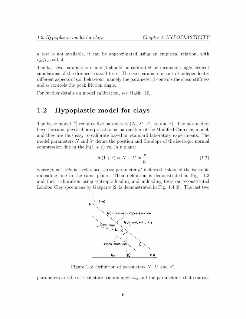
The basic model [7] requires five parameters (N , λ∗, κ∗, ϕc and r). The parametershave the same physical interpretation as parameters of the Modified Cam clay model,and they are thus easy to calibrate based on standard laboratory experiments. Themodel parameters N and λ∗ define the position and the slope of the isotropic normalcompression line in the ln(1 + e) vs. ln p plane:

ln(1 + e) = N − λ∗ lnp

pr. (1.7)

where pr = 1 kPa is a reference stress; parameter κ∗ defines the slope of the isotropicunloading line in the same plane. Their definition is demonstrated in Fig. 1.3and their calibration using isotropic loading and unloading tests on reconstitutedLondon Clay specimens by Gasparre [2] is demonstrated in Fig. 1.4 [9]. The last two

Figure 1.3: Definition of parameters N , λ∗ and κ∗.

parameters are the critical state friction angle ϕc and the parameter r that controls

6

1.3. Intergranular strain concept Chapter 1. HYPOPLASTICITY

the shear stiffness. Due to the non-linear nature of the model, the parameter r needsto be calibrated by simulation of the laboratory experiments. With decreasing valueof r the shear stiffness is increasing (Fig. 1.4b).

Figure 1.4: (a) Calibration of parameters N , λ∗ and κ∗ using isotropic tests onreconstituted London clay, (b) calibration of the parameter r using undrained sheartest on reconstituted London clay (exp. data from Gasparre [2]).

For details of the model for clays with meta-stable structure, see Masın [8]. Calibra-tion procedure is also described in detail in Masın [10].

1.3 The intergranular strain concept (small strain

behaviour)

The intergranular strain concept requires five additional parameters: R controllingthe size of the elastic range, βr and χ controlling the rate of stiffness degradation,mR controlling the initial shear stiffness for the initial and reverse loading conditionsand mT controlling the stiffness upon neutral loading conditions. When combinedwith the hypoplastic model for clays, the initial very-small-strain shear stiffness G0

may be calculated from

G0 'mR

rλ∗p (1.8)

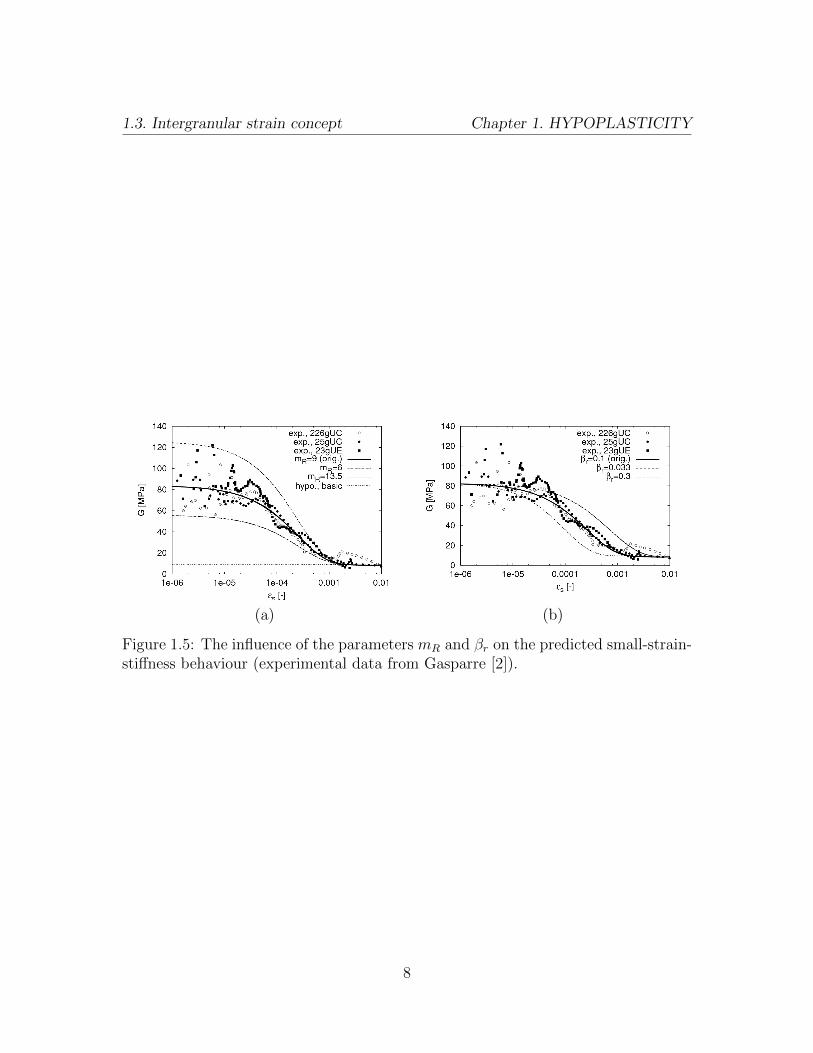
The parameters should be calibrated by simulating the laboratory experiments withmeasurements of the small strain stiffness using local strain transducers and withmeasurements of the very-small-strain stiffness using dynamic methods (such as ben-der elements). The influence of the parameter mR and βr on the predicted small-strain shear stiffness curves is demonstrated in Fig. 1.5.

7

1.3. Intergranular strain concept Chapter 1. HYPOPLASTICITY

(a) (b)

Figure 1.5: The influence of the parameters mR and βr on the predicted small-strain-stiffness behaviour (experimental data from Gasparre [2]).

8

Chapter 2

TIME INTEGRATION

Constitutive models are integrated using explicit adaptive integration scheme withlocal substepping. The constitutive model forms an ordinary differential equation ofthe form

dy

dt= f(t, y)

The equation is for finite time step size ∆t solved using the Runge-Kutta method.Solutions that correspond to the second- and third- order accuracy of Taylor seriesexpansion are given by

y(2)(t+∆t) = y(t) + k2

y(3)(t+∆t) = y(t) +

1

6(k1 + 4k2 + k3)

where

k1 = ∆t f(t, y(t)

)k2 = ∆t f

(t+

∆t

2, y(t) +

k1

2

)k3 = ∆t f

(t+ ∆t, y(t) − k1 + 2k2

)The accuracy of the solution is estimated following Fehlberg as the difference betweenthe second- and third- order solutions. The time step size ∆t is accepted, if

err =∥∥∥y(3)

(t+∆t) − y(2)(t+∆t)

∥∥∥ < TOL

9

Chapter 2. TIME INTEGRATION

where TOL is a prescribed error tolerance. If the step-size ∆t is accepted, y(3)(t+∆t) is

considered as a solution for the given time step and the new time step size ∆tn isestimated according to Hull

∆tn = min

[4∆t, 0.9∆t

(TOL

err

)1/3]

If the step-size ∆t is not accepted, the step is re-computed with new time step size

∆tn = max

[∆t

4, 0.9∆t

(TOL

err

)1/3]

In the case the prescribed minimum time step size or the prescribed maximum num-ber of time substeps is reached, the finite element program is asked to reject thecurrent step and to decrease the size of the global time step.

10

Chapter 3

INPUT OF PARAMETERS ANDSTATE VARIABLES INGEO-SLOPE

3.1 Hypoplastic model for granular materials

Parameters are specified in the GEO-SLOPE input in the following order:

• Parameter 1 (phic) – critical state friction angle ϕc

• Parameter 2 (pt) – pt – shift of the mean stress due to cohesion. The effectivestress σ used in the model formulation is replaced by σ − 1pt. Non-zero valueof pt is needed to overcome problems with stress-free state.

• Parameters 3-9 (hs, nparam, ed0, ec0, ei0, alpha, beta) – parameters of thebasic hypoplastic model for granular materials hs, n, ed0, ec0, ei0, α, β.

• Parameters 10-14 (mR, mT, Rparam, betar, chi) – the intergranular strain con-cept parameters (mR, mT , R, βr, χ). If mR = 0 the intergranular strain conceptis switched off and the problem is simulated using the basic hypoplastic model.

• Parameter 15 (initvoidrat) – initial void ratio corresponding to the zero meanstress e0 or initial void ratio e. If initvoidrat < 10, then e is calculated fromthe mean stress p and from e0 = initvoidrat using Bauer [1] formula. Ifinitvoidrat > 10, then e = initvoidrat− 10.

11

3.2. Hypoplastic model for clays Chapter 3. GEO-SLOPE INPUT

• Parameters 16-19 (istrainxx, istrainyy, istrainzz, istrainxy) – initialvalues of the intergranular strain tensor δ (δ11, δ22, δ33, 2δ12).

Custom Analysis Parameters:

The routine produces 7 custom parameters which can be used for postprocessingpurposes.

• Analysis Custom Param 1-3 – intergranular strain tensor δ components δ11, δ22

and δ12.

• Analysis Custom Param 4 – not used.

• Analysis Custom Param 5 – void ratio e.

• Analysis Custom Param 6 – Number of evaluation of the constitutive model inthe last iteration.

• Analysis Custom Param 7 – Mobilised friction angle ϕmob in degrees.

• Analysis Custom Param 8 – Normalised length ρ of the intergranular straintensor δ.

• Analysis Custom Param 9 – not used.

The hypoplastic model for granular materials is implemented via GEO-SLOPE spe-cific user defined subroutine. To use the model in GEO-SLOPE, copy the implemen-tation into the GEO-SLOPE Add-Ins models directory (specified in Tools→Options).Then, select ”Add-In model” in the ”KeyIn→Materials...” combo box, select ”GeoSlope-Hypo” as an Add-In and ”Hypo Sand Model” as a model. The parameters can thenbe input into the parameter table (Fig. 3.1).

Parameters of the sand hypoplastic model for different soils have been evaluated byHerle and Gudehus [4]. They are given in Table 3.1. Parameters of the intergranularstrain concept for granular materials are in Tab. 3.2.

3.2 Hypoplastic model for clays

Parameters are specified in the GEO-SLOPE input in the following order:

Parameters:

12


Figure 3.1: Selecting sand hypoplasticity model and inputting the parameters.

• Parameter 1 (phic) – critical state friction angle ϕc

• Parameter 2 (pt) – pt – shift of the mean stress due to cohesion. The effectivestress σ used in the model formulation is replaced by σ − 1pt. Non-zero valueof pt is needed to overcome problems with stress-free state.

• Parameters 3-6 (lambdaast, kappaast, Nparam, rparam) – parameters of thebasic hypoplastic model for clays λ∗, κ∗, N , r.

• Parameters 7-9 (kparam, Aparam, sf)– parameters of the model for clays withmeta-stable structure (k, A and sf ).

• Parameters 10-14 (mR, mT, Rparam, betar, chi) – the intergranular strain con-cept parameters (mR, mT , R, βr, χ). If mR = 0 the intergranular strain conceptis switched off and the problem is simulated using the basic hypoplastic model.

• Parameter 15 (Kw) – bulk modulus of water Kw for undrained analysis usingthe penalty approach with user-defined value of Kw. In drained analysis andconsolidation analysis Kw should be set to 0.

13


ϕc hs n ed0 ec0 ei0 α βHochstetten gravel 36◦ 32 ×106 kPa 0.18 0.26 0.45 0.5 0.1 1.9Hochstetten sand 33◦ 1.5 ×106 kPa 0.28 0.55 0.95 1.05 0.25 1.5Hostun sand 31◦ 1.0 ×106 kPa 0.29 0.61 0.96 1.09 0.13 2Karlsruhe sand 30◦ 5.8 ×106 kPa 0.28 0.53 0.84 1 0.13 1Lausitz sand 33◦ 1.6 ×106 kPa 0.19 0.44 0.85 1 0.25 1Toyoura sand 30◦ 2.6 ×106 kPa 0.27 0.61 0.98 1.1 0.18 1.1

Table 3.1: Typical parameters of the hypoplastic model for granular materials (Herleand Gudehus [4])

R mR mT βr χHochstetten sand 1.e-4 5.0 2.0 0.5 6

Table 3.2: Parameters of the intergranular strain concept for sandy soils (Niemunisand Herle [12])

• Parameter 16 (initvoidrat) – initial void ratio e or overconsolidation ratioOCR. If initvoidrat < 10, then e = initvoidrat. If initvoidrat > 10,then OCR = initvoidrat− 10.

• Parameter 17 (sens) – initial value of sensitivity (model for clays with meta-stable structure). If s = 0, the basic model is used.

• Parameters 18-21 – (istrainxx, istrainyy, istrainzz, istrainxy) – initialvalues of the intergranular strain tensor δ (δ11, δ22, δ33, 2δ12).

Custom Analysis Parameters:

The routine produces 9 custom parameters which can be used for postprocessingpurposes.

• Analysis Custom Param 1-3 – intergranular strain tensor δ components δ11, δ22

and δ12.

• Analysis Custom Param 4 – Excess pore pressure u for undrained analysis usinguser-defined value of Kw.

• Analysis Custom Param 5 – void ratio e.

14


• Analysis Custom Param 6 – Number of evaluation of the constitutive model inthe last iteration.

• Analysis Custom Param 7 – Mobilised friction angle ϕmob in degrees.

• Analysis Custom Param 8 – Normalised length ρ of the intergranular straintensor δ.

• Analysis Custom Param 9 – sensitivity s (for model with meta-stable struc-ture).

The hypoplastic model for clays is implemented via GEO-SLOPE specific user definedsubroutine. To use the model in GEO-SLOPE, copy the implementation into theGEO-SLOPE Add-Ins models directory (specified in Tools→Options). Then, select”Add-In model” in the ”KeyIn→Materials...” combo box, select ”GeoSlopeHypo” asan Add-In and ”Hypo Clay Model” as a model. The parameters can then be inputinto the parameter table (Fig. 3.2).

Figure 3.2: Selecting clay hypoplasticity model and inputting the parameters.

Parameters of the clay hypoplastic model for different soils have been evaluatedby Masın and co-workers. They are given in Table 3.3. Parameters of the model

15


for clays with meta-stable structure are in Tab. 3.4 and typical parameters of theintergranular strain concept for fine-grained soils are in Tab. 3.5.

ϕc λ∗ κ∗ N rLondon clay 22.6◦ 0.11 0.016 1.375 0.4Brno clay 19.9◦ 0.13 0.01 1.51 0.45Fujinomori clay 34◦ 0.045 0.011 0.887 1.3Bothkennar clay 35◦ 0.12 0.01 1.34 0.07Pisa clay 21.9◦ 0.14 0.01 1.56 0.3Beaucaire clay 33◦ 0.06 0.01 0.85 0.4Kaolin 27.5◦ 0.11 0.01 1.32 0.45London clay. (data Gasparre) 21.9◦ 0.1 0.02 1.26 0.5Kaolin 27.5◦ 0.07 0.01 0.92 0.67Trmice clay 18.7◦ 0.09 0.01 1.09 0.18

Table 3.3: Typical parameters of the hypoplastic model for clays

k A sfPisa clay 0.4 0.1 1Bothkennar clay 0.35 0.5 1

Table 3.4: Typical parameters of the model for clays with meta-stable structure

R mR mT βr χLondon clay [7] 1.e-4 4.5 4.5 0.2 6London clay (data Gasparre) 5.e-5 9 9 0.1 1Brno clay (nat.) 1e-4 16.75 16.75 0.2 0.8

Table 3.5: Typical parameters of the intergranular strain concept for clays

16

Chapter 4

COMMENTS ON THEIMPLEMENTATION

4.1 Initial conditions

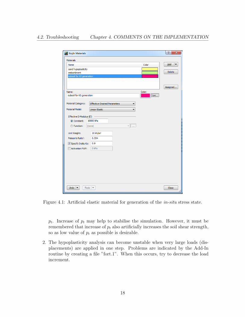
The initial stress field is generated in the analysis phase which precedes the hypoplas-tic analysis. As it is not possible to specify K0 value for the Add-In model, the area ofthe hypoplastic material must for the initialisation be filled with artificial elastic soil.Using this material, it is possible to specify K0 for the ”Insitu” analysis type (see Fig.4.1). Then, in the first hypoplastic phase, the model takes over stresses generated inthe in-situ phase and intialises the other state variables (void ratio/OCR, sensitivity,intergranular strain tensor) using values specified in the parameters table.

4.2 Troubleshooting

Although the implementation has been tested to be accurate and robust, the hy-poplastic models are highly non-linear which may cause problems during solvingcomplex boundary value problems. When encountering problems, the following stepsmay help to improve the overall performance:

1. The hypoplastic models are undefined in the tensile stress region, which cancause integration problems in the vicinity of the free surface and in the case ofstaged construction starting from the stress-free state. For this reason, artificialcohesion is introduced in the model implementation through the parameter

17

4.2. Troubleshooting Chapter 4. COMMENTS ON THE IMPLEMENTATION

Figure 4.1: Artificial elastic material for generation of the in-situ stress state.

pt. Increase of pt may help to stabilise the simulation. However, it must beremembered that increase of pt also artificially increases the soil shear strength,so as low value of pt as possible is desirable.

2. The hypoplasticity analysis can become unstable when very large loads (dis-placements) are applied in one step. Problems are indicated by the Add-Inroutine by creating a file ”fort.1”. When this occurs, try to decrease the loadincrement.

18

4.3. Postprocessing Chapter 4. COMMENTS ON THE IMPLEMENTATION

4.3 Postprocessing

Several variables are available for postprocessing as ”Custom Analysis Parameters”.Their meaning is demonstrated using the snapshots from the analysis of rigid footingand an embankment.

19


Figure 4.2: Intergranular strain component δ22 is under the ”Analysis Custom Param2”.

Figure 4.3: Intergranular strain shear component δ12 is under the ”Analysis CustomParam 3”.

20


Figure 4.4: The length of the intergranular strain tensor ρ is under the ”AnalysisCustom Param 8”. When ρ = 1 the material is swept out of the small strain memory.Contrary, when ρ = 0 (this often coincides with the initial condition), the soil is insideits very-small-strain elastic range.

Figure 4.5: ”Analysis Custom Param 5” represents the actual void ratio.

21


Figure 4.6: ”Analysis Custom Param 7” represents the mobilised friction angle. Thisquantity gives us an indication how far the soil is from the failure state.

22


Figure 4.7: ”Analysis Custom Param 6” (ACP6) indicates how many times the con-stitutive model was called in one iteration within the RKF23 integration schemewith adaptive substepping. Its value divided by three gives us the actual number ofsubsteps (thus ACP6=3 is a minimum value). Very large values of ACP6 (severalhundreds and more) indicate the global step is too large, its decrease is then recom-mended for the overall stability of the simulation. The pattern of the ACP6 oftencorresponds to the size of the strain increment, but other factors also come into play(distance from the stress limitting condition etc.)

23

REFERENCES

[1] E. Bauer. Calibration of a comprehensive constitutive equation for granularmaterials. Soils and Foundations, 36(1):13–26, 1996.

[2] A. Gasparre. Advanced laboratory characterisation of London Clay. PhD thesis,University of London, Imperial College of Science, Technology and Medicine,2005.

[3] G. Gudehus. A comprehensive constitutive equation for granular materials. Soilsand Foundations, 36(1):1–12, 1996.

[4] I. Herle and G. Gudehus. Determination of parameters of a hypoplastic constitu-tive model from properties of grain assemblies. Mechanics of Cohesive-FrictionalMaterials, 4:461–486, 1999.

[5] I. Herle and D. Kolymbas. Hypoplasticity for soils with low friction angles.Computers and Geotechnics, 31(5):365–373, 2004.

[6] D. Kolymbas. Computer-aided design of constitutive laws. International Journalfor Numerical and Analytical Methods in Geomechanics, 15:593–604, 1991.

[7] D. Masın. A hypoplastic constitutive model for clays. International Journal forNumerical and Analytical Methods in Geomechanics, 29(4):311–336, 2005.

[8] D. Masın. A hypoplastic constitutive model for clays with meta-stable structure.Canadian Geotechnical Journal, 44(3):363–375, 2007.

[9] D. Masın. 3D modelling of a NATM tunnel in high K0 clay using two differentconstitutive models. Journal of Geotechnical and Geoenvironmental EngineeringASCE, 135(9):1326–1335, 2009.

[10] D. Masın. Hypoplasticity for practical applications – PhD course.http://web.natur.cuni.cz/uhigug/masin/hypocourse, 2010.

24

REFERENCES REFERENCES

[11] A. Niemunis. Extended Hypoplastic Models for Soils. Habilitation thesis, Ruhr-University, Bochum, 2003.

[12] A. Niemunis and I. Herle. Hypoplastic model for cohesionless soils with elasticstrain range. Mechanics of Cohesive-Frictional Materials, 2:279–299, 1997.

[13] P. A. von Wolffersdorff. A hypoplastic relation for granular materials witha predefined limit state surface. Mechanics of Cohesive-Frictional Materials,1:251–271, 1996.

25

geo-slope sigma/w implementation of hypoplasticity · di erent aspects of soil behaviour, namely...

Documents